http://wrap.warwick.ac.uk/
Original citation:
Black, Andrew J., House, Thomas A., Keeling, Matthew James and Ross, Joshua V..
(2014) The effect of clumped population structure on the variability of spreading
dynamics. Journal of Theoretical Biology, Volume 359 . pp. 45-53.
Permanent WRAP url:
http://wrap.warwick.ac.uk/62714
Copyright and reuse:
The Warwick Research Archive Portal (WRAP) makes this work of researchers of the
University of Warwick available open access under the following conditions. Copyright ©
and all moral rights to the version of the paper presented here belong to the individual
author(s) and/or other copyright owners. To the extent reasonable and practicable the
material made available in WRAP has been checked for eligibility before being made
available.
Copies of full items can be used for personal research or study, educational, or
not-for-profit purposes without prior permission or charge. Provided that the authors, title and
full bibliographic details are credited, a hyperlink and/or URL is given for the original
metadata page and the content is not changed in any way.
Publishers statement:
NOTICE: this is the author’s version of a work that was accepted for publication in
Journal of Theoretical Biology. Changes resulting from the publishing process, such as
peer review, editing, corrections, structural formatting, and other quality control
mechanisms may not be reflected in this document. Changes may have been made to
this work since it was submitted for publication. A definitive version was subsequently
published in Journal of Theoretical Biology, Volume 359 . pp. 45-53.
http://dx.doi.org/10.1016/j.jtbi.2014.05.042
A note on versions:
The version presented here may differ from the published version or, version of record, if
you wish to cite this item you are advised to consult the publisher’s version. Please see
the ‘permanent WRAP url’ above for details on accessing the published version and note
that access may require a subscription.
The e
ff
ect of clumped population structure on the variability of spreading dynamics
Andrew J. Blacka,∗, Thomas Houseb,c, M. J. Keelingb,c,d, J. V. Rossa
aSchool of Mathematical Sciences, The University of Adelaide, Adelaide SA 5005, Australia. bMathematics Institute, Zeeman Building, University of Warwick, Gibbet Hill Road, Coventry CV4 7AL, UK.
cWarwick Infectious Disease Epidemiology Research (WIDER) Centre, University of Warwick, Gibbet Hill Road, Coventry CV4 7AL, UK. dSchool of Life Sciences, University of Warwick, Gibbet Hill Road, Coventry CV4 7AL, UK.
Abstract
Processes that spread through local contact, including outbreaks of infectious diseases, are inherently noisy, and are frequently observed to be far noisier than predicted by standard stochastic models that assume homogeneous mixing. One way to reproduce the observed levels of noise is to introduce significant individual-level heterogeneity with respect to infection processes, such that some individuals are expected to generate more secondary cases than others. Here we consider a population where individuals can be naturally aggregated into clumps (subpopulations) with stronger interaction within clumps than between them. This clumped structure induces significant increases in the noisiness of a spreading process, such as the transmission of infection, despite complete homogeneity at the individual level. Given the ubiquity of such clumped aggregations (such as homes, schools and workplaces for humans or farms for livestock) we suggest this as a plausible explanation for noisiness of many epidemic time series.
Keywords: epidemics, continuous-time Markov chain, offspring distribution, diffusion approximation
1. Introduction
Processes that spread between individuals in a population have, under various guises, been extensively studied and applied to many biological and physical problems (Boccaletti et al., 2006; Danon et al., 2011). It has been noticed for some time that many models of these processes do not capture
the noisy behaviour of empirical data. For example many
epidemic outbreaks are far noisier than predicted by simple models (Watts et al., 2005), suggesting that some element (or elements) are missing from these.
This enhanced variability has several important implications for the dynamics, especially during the early stages of invasion. Most notably, early extinctions will be far more common than anticipated from a birth-death process, and we may expect to observe several small outbreaks before the number of cases becomes large. This latter phenomenon has been observed in several real epidemics, as for example in the case of SARS
in 2002–2003 (Anderson et al., 2004). Another possible
explanation for such stuttering chains is due to a change in
transmissibility due to evolutionary factors, such that the basic reproduction number, R0, transitions from below one to
above one (Lloyd-Smith et al., 2009). This phenomenon has been identified as an evident gap in modelling and a natural question arises of whether, in a given outbreak, stuttering is a consequence of evolutionary factors or simply a result of natural variability (Lloyd-Smith et al., 2009). Obviously,
∗
Corresponding author: School of Mathematical Sciences, The University of Adelaide, Adelaide SA 5005, Australia. Phone:+61883134177
Email address:[email protected](Andrew J. Black)
once many individuals are infected, the relative impact of the
noise is reduced. Still, fully accounting for the variability
is important in order to better inform decision making, for example via uncertainty analyses which capture the extent of probabilistic uncertainty surrounding the effectiveness of inter-ventions (Black et al., 2013; Gilbert et al., 2014). Therefore understanding and capturing this larger-than-expected noise is of fundamental public-health importance in terms of un-derstanding invasion, persistence and eradication of infection. Incorrect assumptions could substantially bias our parameter inferences (and hence predictions) from early outbreak data.
that power-law like degree distributions that allow large third moments but modest second moments, are considered by some to be unrealistic representations of real social transmission
networks (Clauset et al., 2009). Another objection is that
this approach would necessitate afine tuningof moments that
would need to hold forallnetworks exhibiting significant noise in spreading dynamics.
A question of both theoretical and applied interest is whether greater variability can be replicated with a simpler and more robustly tuneable model. Here we rely on the natural aggrega-tion (clumping) of individual hosts and consider a model with two-levels of mixing – within-clumps and between-clumps – but where all individuals are homogeneous; that is, all individ-uals are identical, but there are differential rates of transmission, high within a clump and low between clumps. Specifically,
we consider a population made up ofN = m×nindividuals,
in a total of m clumps each of size n, which we index with
i=1, . . . ,m. We consider a stochastic epidemic process on this population: clumpihasSisusceptibles and Iiinfectives, such thatSi+Ii≤n. The rates of this process are:
(Si,Ii)→(Si−1,Ii+1), at rateSi
βIi
(n−1)+
α N
m
X
j=1
Ij
;
(Si,Ii)→(Si,Ii−1) , at rateγIi, (1)
where β is the effective within-clump transmission rate
pa-rameter, α is the effective between-clump transmission rate
parameter and γis the per-infective recovery rate. Note that
frequency-dependenttransmission is used in Eq. (1). Another common choice is density-dependent transmission whereβis not scaled by the factor 1/(n−1). We do not present results for this form of transmission as it allows for unrealistically large within-clump transmission, but we do discuss how our results are changed by this.
We wish to consider the limit as the number of patches,m,
becomes large but where the patch size, n, remains finite and
often relatively small. Note that for such a population structure, individuals are homogeneous, and the network topology (de-fined by within and between clump contact rates) also exhibits the desirable ‘small worlds’ property of high clustering and low shortest path lengths (Travers and Milgram, 1969; Watts and Strogatz, 1998). Many real-world populations exhibit this clumped population structure, where strong links exist within a clump and weaker links exist between clumps. High-profile examples include the transmission of avian influenza in poultry aggregated into sheds (Savill et al., 2006), spread of Foot-and-Mouth disease in livestock aggregated into farms (Tildesley et al., 2006), transmission of measles by children aggregated into schools (Riley et al., 1978), and the spread of a number of infections such as pandemic influenza through human populations that are aggregated into households (Black et al., 2013). For this type of clumped population, expressions for the probability of a major outbreak (successful invasion) and the final size of an epidemic (and hence results for percolation as a
special case) have been derived (Ball et al., 1997).
Our aim is to assess the variability of spreading in this clumped population during the early phase of an epidemic be-fore there is a significant depletion of susceptible clumps in the overall population. Within this early phase we can identify two
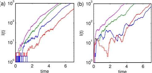
dynamical regimes (see Figure 1). (i) Initial behaviour: Here
the epidemic dynamics are well approximated by a
branch-ing process between clumps. (ii) Early asymptotic behaviour:
After a significant number of between-household transmission events, the proportion of infected individuals becomes signifi-cant and the mean prevalence of infection,hI(t)i, grows expo-nentially with fixed,early growthrater,
hI(t)i ∝ert. (2)
Figure 1 shows stochastic simulations of this process to illustrate the dynamics of the two regimes. Figure 1(a) shows
typical dynamics from a random-mixing model (n =1) while
Figure 1(b) shows dynamics from the clumped model (n=20).
During the initial phase (i) clumping of the population mainly affects the variability in the timing of the start of the exponential growth phase, often giving rise to stuttering dynamics. Using the branching process approximation, we calculate a number of quantities which allows us to understand how the variability changes across clump sizes and within-clump transmission rates. To investigate the variability in stage (ii)we derive an analytic diffusion approximation to calculate the variance in the infectious process (Kurtz, 1970, 1971).
0 2 4 6
100 101 102 103
time
I(t)
0 2 4 6
100 101 102 103
time
I(t)
[image:3.595.309.556.459.578.2](a) (b)
Figure 1: Stochastic simulations of the process Eq. (1) illustrating the early time behaviour and the two dynamical regimes withn=1 (a) andn=20 (b). The variability in the first phase mainly affects the timing of the second, exponential phase. Parameters:m=104,β=20,r=1.
To maintain a fair comparison across clump sizes, n, and
within-clump transmission rates,β, we calculate all quantities for the same early growth rate, which we fix arbitrarily as
r=1. For given values ofβandnwe scale the between-clump
transmission rate,α, to achieve this. There is another quantity which we could instead fix: the clump reproductive ratioR∗, which is the expected number of secondary clumps infected by a primary clump (Ball et al., 1997; Ross et al., 2010). We note that these two quantities are linked (Svensson, 2007; Wallinga and Lipsitch, 2007) and we chose to fix r instead
of R∗ because the early growth rate is most easily estimated from data. Throughout this paper we also fix the recovery rate atγ=1, which can be done without loss of generality by rescaling time.
2. Initial behaviour
During this phase the epidemic dynamics are well ap-proximated by a branching process between clumps (Ball et al., 1997; Ross et al., 2010). The within-clump dynamics
are modelled as a continuous-time Markov chain, X(t), with
transition rate matrixQ=(qi j;i,j∈S). The transition rates are as in Eq. (1) withα=0 andqii=−P
j∈Sqi j. The state space is S =A∪C, whereCis an irreducible set of transient states (all possible states of a clump with I >0 andS +I ≤n) andAis the set of absorbing states (corresponding toI =0) within the clump. The functionI(X(t)) then gives the number of infected
individuals within a clump at time t. New clumps are then
infected according to a Poisson process with time-dependent rateαI(X(t)).
The growth rate of the process,r, is defined by the equation (Ball et al., 1997),
E
"Z ∞
0
αI(X(t))e−rtdt
#
=1. (3)
The left-hand-side of Eq. (3) can be efficiently evaluated numer-ically using exponential discounting (Ross et al., 2010). Com-bined with a basic root finding algorithm, this allows us to eas-ily compute r. All results are derived by finding the value of
αwhich givesr =1 for a given clump size and within-clump
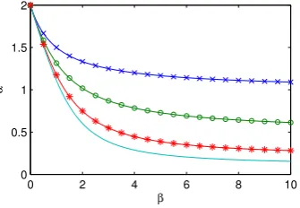
transmission rateβ. Figure 2 shows contours of constantrfor different sized clumps. This extends to larger values ofβthan αas it is typically assumed that the within-clump transmission rate will be larger than the between-clump transmission rate.
0 2 4 6 8 10
0 0.5 1 1.5 2
β
[image:4.595.82.250.536.652.2]α
Figure 2: Values ofαandβwhich give the same early growth rate,r =1. Clump sizes are: 2, 4, 10 and 20 (crosses, circles, stars and plain line respec-tively).
By fixing the mean growth rate for all clump sizes and pa-rameters, the mean number of infected individuals in the early stages of the epidemic is also fixed. The spreading dynamics will be an interplay of the within-clump and the between-clump dynamics and hence, although the mean growth rate remains
fixed, there can be a large change in the variability of the process with different parameters. This variability in the initial stages of the branching process is crucial for understanding the variability in the numbers of patches infected and hence
the probability of a major outbreak (or, disease extinction)
and the timing of the start of the exponential growth phase. Intuitively, more variability will lead to a greater probability of extinction and a larger variability in the timing of the start of the exponential phase.
To understand how the variability of the spreading process changes with clump size and other parameters we calculate three main quantities. The first is the offspring distribution, de-noted byh(m). This is the probability distribution of the number of secondary clumps infected by a primary clump. This will be Poisson with a random mean,
h(m)=
Z ∞
0 ρ(b)e
−bbm
m! db, (4)
whereρ(b) is the probability density function corresponding to the random variableβ=R αI(X(t))dt, which is the total force of external infections created by a clump. Previous work has detailed how the offspring distribution can be efficiently calcu-lated (Ross et al., 2010). The mean of the offspring distribution is then justR∗, the expected number of secondary clumps in-fected by a primary. Alternatively,R∗ can be calculated more efficiently using path integral techniques, (Pollett and Stefanov, 2002; Ross et al., 2010)
R∗=E
"Z ∞
0
αI(X(t))dt
#
. (5)
The second quantity we calculate is the time to first infection of a secondary clump, conditioned on there being such an infection, which we denote byτand henceforth refer to as the conditional first infection time. In Appendix A we detail how this can be calculated efficiently.
The last quantity we consider is the final size distribution within a clump. This is the probability distribution that a given proportion of the clump will have been infected over the course of the within-clump epidemic. This can be calculated via a number of methods (Ball, 1986; House et al., 2013).
2.1. Results
conditional first infection time. Finally, the mean and variance of the final size distribution, as a function of β and n, is shown in Figure 5. Here the mean increases monotonically with both n and β, whereas the variance is non-monotonic. Taken together, Figures 3, 4 and 5 show that there is a complex interplay between the spread of the disease between the clumps and the within-clump dynamics which changes significantly as the clump size and transmission rates are varied.
In deciphering the dynamics of this branching process it helps to consider the two different types of scaling that are possible. The most natural, and of primary interest for this paper, is keeping βfixed while increasing the clump size n. A basic consequence of this is that for larger n, less clumps contribute to the overall prevalence, hence if the within clump dynamics are noisy, so will the overall dynamics. Another scaling is to hold n fixed and vary β. This is a less natural situation as the extremes are somewhat unphysical, but it can aid our understanding of the dynamics.
As it is independent ofα, the easiest aspect to understand is the within-clump dynamics and hence the final size distribu-tion. The mean and variance are shown in Figure 5 along with the actual distributions for three values ofβ. Firstly, given that
γ =1, it is required thatβ > 1 for a large epidemic within the clump to occur. This sets a threshold for an epidemic, although we can see that even for β < 1 there is some probability of multiple infections within the patch. As βis increased, large epidemics become possible and the final size distribution becomes strongly bimodal. This can be seen clearly in the variance which is non-monotonic. Importantly, the time-scale of the within-clump epidemic decreases asβis increased. At the extreme, as β → ∞ then the clump increasingly acts as one unit, such that after the initial infection the whole clump becomes infected very quickly (this fact is used to derive an approximation in the next section of the paper.) The variance then decreases as the probability of no further infection decreases.
Understanding the changes in the offspring and conditional first infection time distribution follow on from the within-clump dynamics. As larger within-within-clump epidemics become possible, thenR∗also increases as a clump can potentially give rise to more external infections. The bi-modality in the final size distribution then accounts for the rise in the variance in the offspring distribution. For a large enough value ofβ, increasing nleads to a linear increase in the proportion of the clump that becomes infected. An important point here is, that because we hold rfixed, an increase in R∗ must be offset by an increase in the time between clump infections, hence why Figure 4 shows an increase in the mean time to first infection. When
β → ∞ the mean time a patch is infectious for is controlled almost completely by the recovery process as the whole clump becomes infectious straight after initial infection.
Multiple components of the behaviour illustrated in Figures 3-5 drive the early stochastic dynamics. When βand n are
n
β
5 10 15 20
0 2 4 6 8 10
2 3 4 5
n
β
5 10 15 20
0 2 4 6 8 10
10 20 30 40
[image:5.595.308.558.81.178.2](a) (b)
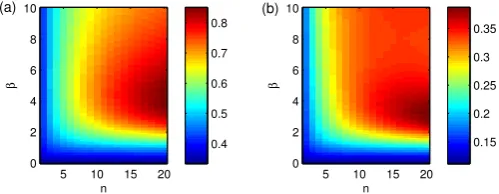
Figure 3: The mean (a) and variance (b) of the offspring distribution. The mean is equal toR∗.
n
β
5 10 15 20
0 2 4 6 8 10
0.4 0.5 0.6 0.7 0.8
n
β
5 10 15 20
0 2 4 6 8 10
0.15 0.2 0.25 0.3 0.35
(a) (b)
Figure 4: The mean (a) and variance (b) ofτ, the conditional time to first infec-tion.
large (and hence α is small to maintain r = 1, Figure 2), the within-clump dynamics are characterised by rapid spread that generally infects the vast majority of the clump within a short period of time (Figure 5). Yet the mean time to infect another clump is relatively long with high variance (Figure 4). Therefore we are likely to see saw-tooth aggregate dynamics, where the level of infection in one clump starts to decline before other clumps are infected. A secondary effect predominates at intermediateβ (and highn), due to the high variance in within-clump final size (Figure 5) – which in turn generates high variance in both the offspring distribution and conditional time to first infection (Figures 3 and 4). These high variances combine to give long (and variable) periods between the seeding of infection and the onset of sustained exponential growth once a significant number of clumps are infected. Together these two elements of highly variable dynamics and rapid within-clump dynamics compared to between-clump transmission, explain the early behaviour observed in Figure 1(b).
3. Early asymptotic behaviour
After transmission has become established, but before there has been an appreciable depletion of susceptible clumps, the
mean prevalence of infection grows exponentially.The
branch-ing process discussed in the previous section is still valid and would allow us to calculate the variance in the overall number of infected but the method is problematic to implement (Ner-man, 1981; Ball and Donnelly, 1995). Instead, weinvestigate this phase of the epidemic by deriving a diffusion approxima-tion for the process in the limit of the number of clumpsm→ ∞
[image:5.595.307.557.223.320.2]n
β
5 10 15 20
0 2 4 6 8 10
5 10 15
n
β
5 10 15 20
0 2 4 6 8 10
0 20 40 60
0 5 10 15
0 0.2 0.4 0.6 0.8
final size
probability
0 5 10 15
0 0.1 0.2 0.3 0.4
final size
0 5 10 15
0 0.2 0.4 0.6 0.8 1
final size
(a) (b)
[image:6.595.41.289.81.258.2](c) (d) (e)
Figure 5: The mean (a) and variance (b) of the final size distribution for the within-clump epidemic. Parts (c), (d) and (e) show the final size distribution for a clump size of 15 withβ=0.8, 3 and 8 respectively. The variance tends to decrease as we increaseβpast this threshold as large outbreaks become more probable. For a large value ofβincreasing the clump size just increases the proportion who become infected.
(Kurtz, 1970, 1971). This is a perturbative expansion in m−1,
the inverse number of clumps, which allows us to approximate the full stochastic dynamics with a deterministic part, describ-ing the mean behaviour, plus a stochastic correction (van Kam-pen, 1992; Black and McKane, 2011). From this we can calcu-late the variance in the total prevalence of infection. The details of this calculation are given in Appendix B, but are summarised here. Asymptotically, we find that
Var(I(t))→ve2rt, (6)
where v is independent of time. As we fix r = 1 for all
calculations, the variation induced by the clumping comes entirely from the multiplicative factor v. This gives the size of the envelope around the mean in which typical stochastic realisations lie.
Of particular interest is how the variance (Eq. (6)) increases with clump size,n, for fixed values of within-clump
transmis-sion,β. In the limit β → ∞we can derive an expression for
the variance by assuming that each between clump transmis-sion leads to rapid (instantaneous) infection of the entire clump; this is therefore equivalent of a standard SIR model where each transmission event causes a change of magnitudenin the global susceptible and infected population sizes:
(S,I)→(S −n,I+n). (7)
In this limiting case, and using the same steps as for the full
model, we find that the factor v increases linearly with the
clump sizen,
v=n(r+γ)+γ
r . (8)
Again, full details of this calculation are given in Appendix C.
n
β
5 10 15
0 5 10 15 20
1 2 3 4 5 x 10⁻⁴
n
β
5 10 15
0 5 10 15 20
0.5 1 1.5 2 2.5 x 10⁻⁴
0 5 10 15 20
0 2 4 6 8x 10
−4
n
v
(b) (a)
[image:6.595.310.552.82.278.2](c)
Figure 6: The asymptotic early value ofv=hI2ie−2rtas a function of the clump size,n, and the within-clump transmission parameter,β, assuming density-dependent transmission (a) and frequency-density-dependent transmission (b). Density dependent transmission assumes that the transmission rateβisnotscaled by the factor 1/(n−1). Panel (c) showsvas a function ofnforβ=20. The green line is the asymptotic result from Eq. (8). The blue and red points assume density-and frequency-dependent transmission respectively.
Figure 6 shows numerical results forvas a function of the
clump size,n, and within-clump transmission rate. As we fix
r=1 throughout, then the mean overall level of infection grows
at the same rate for all parameters. Here we consider both
frequency-dependent transmission as in the previous section, and also density-dependent transmission, whereβis not scaled by the factor 1/(n−1). Density-dependent transmission allows for much larger transmission rates within a clump and so is a better comparison with the limiting case, (8), whereβ → ∞.
Figure 6 shows that, as in the very early stages, changes in clump size alone can induce large differences in the variability of the spreading process. In contrast to the early stages, the vari-ance increases monotonically with both clump size and
within-clump transmission rate. Figure 6(c) shows howvchanges with
clump size for a fixed value of transmission parameterβ, and
also includes the theoretical limit from Eq. (8), which is a linear increase withn. For finite values ofβthe increase in variance is always sub-linear.
4. Discussion and Conclusion
epidemics (Anderson et al., 2004; Watts et al., 2005). Com-bined with partial detection of cases, this could be mistaken as stochastic fade-out followed by re-introductions of infection.
In Section 2 we presented results using what is know as frequency-dependent transmission where the transmission rate parameter,β, is scaled by 1/(n−1). Another common choice is density-dependent transmission whereβis not scaled. In terms of our model, frequency-dependent transmission is the most realistic scenario, as within-clump transmission rates cannot become too large. Using density-dependent transmission means that large clumps have much stronger rates of infection, leading to larger / faster outbreaks, due to their increased number of susceptible individuals. In terms of our results in Section 2, the more extreme within-clump dynamics which results from assuming density dependent transmission means the window where we observe interesting population level dynamics is much reduced. In Section 3 we do present results using density-dependent transmission. This is primarily to compare with the analytic β → ∞limit, which is obviously easier to achieve whenβis not scaled by 1/(n−1).
All of the methods used to analyse the dynamics in stage (i) can be naturally extended to more realistic models such
as SE2I2R – that is the model considered here extended to
have Erlang-2 distributed exposed and infectious periods, more clearly reflecting the shape of the true distributions – which has been used for pandemic influenza studies (Black et al., 2013). This involves using larger stochastic matrices, so there is a computational cost, but because most of our methods only rely on solving linear sets of equations, they scale efficiently.
Our model is clearly related to meta-population models, that have been considered previously as models of infection spread in aggregated populations (Lloyd and May, 1996; Riley and others, 2003; Rozhnova et al., 2012). The novelty in our work is that we consider a different population level limit – meta-populations often are considered as a small number of large clumps (for example representing cities in a country), where as we consider a large number of small clumps (more reminiscent of households within a country). Taking this limit of a large number of clumps means we can analyse the variability in the early growth phase (ii) using a diffusion approximation, but currently this does have limitations, most obviously in the range of clump sizes for which we can explicitly calculate the variance. This is due to numerical errors in calculating the eigenvectors of the Jacobian matrix, which in turn are used to expand a matrix exponential, Eq. (B.13). In practice, clump sizen =16 was the largest value we could use over the entire range of the other parameters. It is possible that a different approach to evaluating the coefficients of this expansion would allow us to go to higher values ofn. It is possible to extend the diffusion approximation result to heterogeneous populations, but the usefulness of this is questionable. For example, the results will depend on the proportions of each size of clump and this has to be incorporated via careful choice of initial conditions.
To conclude, we have shown that a simple model, which involves a very generic structure and relatively little parame-ter tuning can reproduce real-world features as has only been demonstrated with highly heterogeneous approaches to date. It has also uncovered a number of interesting features which war-rant further investigation.
Acknowledgements
This research was supported under the Australian Research Council’s Discovery Projects funding scheme (project number DP110102893) (AJB & JVR) and the UK Engineering and Physical Sciences Research Council (TH & MJK). MJK and JVR also received support from the Royal Society (Interna-tional Exchanges Scheme). We would like to thank the two anonymous referees who’s comments have substantially im-proved this paper.
Appendix A. Initial behaviour methodology
Offspring distribution
The offspring distribution, denoted byhi(m), is the probabil-ity mass function of the number of secondary clumps infected by a primary clump conditional on starting in statei. This will be Poisson with a random mean,
hi(m)=
Z ∞
0 ρ(b)e
−bbm
m! db, (A.1)
whereρ(b) is the probability density function corresponding to the random variableβ = R αI(X(t)|X(0) = i)dt, which is the total force of external infection created by a clump. We evaluate the offspring distribution as detailed in (Ross et al., 2010).
Conditional first infection time
Next we wish to calculate the mean and variance ofτ, the conditional first time to infection. This uses basic theory of Markov processes (Waugh, 1958; Norris, 1997).
First, we augment the original Markov chain, representing the within-clump dynamics, with a third variable, a, which counts the number of external infections caused by the clump. The transition rates for this new chain are then,
(S,I,a)→(S −1,I+1,a), at rate βS I (n−1) (S,I,a)→(S,I,a+1), at rate αI
(S,I,a)→(S,I−1,a), at rate γI
(A.2)
Next we condition theQmatrix on observing at least 1 external infection, i.e. a >0. This involves modifying the elements of the transition matrixQ(Waugh, 1958):
¯ qi j= uj
ui
!
qi j, (A.3)
for all statesifrom whichui>0 and ¯qi j =qi jotherwise, where ui is the probability of at least 1 external infection given that
the process starts from statei. These probabilities correspond to the complementary probability of no further infections, avail-able from the offspring distribution, as detailed earlier, starting from each statei; that is,ui =1−hi(0). Finally, we make the states of the system corresponding toa =1 absorbing by set-ting the relevant elements of ¯qi jequal to zero. The mean of the conditional first infection time starting from state j,hτij, is then found by solving a set of linear equations (Norris, 1997),
X
j∈C ¯
qi jhτij=−1. (A.4)
The second moment can be found from,
X
j∈C ¯
qi jhτ2ij=−2hτii, (A.5)
which allows us to calculate the variance.
Appendix B. Diffusion approximation for exponential growth phase
Before we go into the details of this calculation, we give a brief outline of the various steps. The first step is to show that the stochastic process is of the correct form, so that we can derive a diffusion approximation in the limit that the number of clumps, m → ∞. Once this is done we then apply the ap-proximation to our system, giving equations for the mean and variance of theproportionsof the clumps of each type. Finally, we describe how these equations can be approximately solved when we consider just the early time dynamics. This is valid in the period of time between when the exponential growth starts and before the peak in the epidemic.
Diffusion approximation
We defineHx,y(t) as the number of clumps withxsusceptible andyinfected at timet. The state of the system is then defined asH(t)={Hx,y(t)|x+y≤n}wherenis the size of the clumps.
This is equivalent to the original process, but reduces the
num-ber of variables in the problem from 2mto (n+1)(n+2)/2.
In this representation an infection or recovery event results in a clump in the current configuration being replaced by a clump with the updated configuration. The total number of infected in-dividuals across all clumps is given byY(t)=y·H(t), wherey
gives the number of infected in each clump configuration. The transition rates for this new process are then,
(Hx,y,Hx,y−1)→(Hx,y−1,Hx,y−1+1)
at rateγyHx,y, (Hx,y,Hx−1,y+1)→(Hx,y−1,Hx−1,y+1+1)
at ratexHx,y(βy+αY(t)) .
(B.1)
We next define the proportion of clumps in each configura-tion, φx,y(t) =m−1Hx,y(t), and the overall proportion infected, I(t) = (nm)−1Y(t). From herein we drop the dependence on
time of theHx,yandφx,yfor clarity.The two transmission rates
can then be written as
γyHx,y=myγφx,y,
xHx,y(βy+αY(t))=mxφx,y(βy+αI(t)) .
(B.2)
These are of the correct form for a density-dependent Markov chain, and the results of Kurtz give a simple procedure for
de-riving the diffusion approximation (Kurtz, 1970, 1971). The
same results can be obtained from a linear-noise approximation or a WKB approximation (van Kampen, 1992; Black and McK-ane, 2011).
To leading orderin the diffusion approximation, the propor-tions of clumps in each configuration is given by a set of ODEs,
˙
φ=F= X
µ=1,2
lµwµ. (B.3)
where (w1)i =γyiφiand (w2)i =(αI(t)+βyi)xiφiThe two
ma-triceslµencode all the recovery (µ=1) and infection (µ=2) events respectively. The elements of these are
(l1)i j=−δyi,yj+δxi,xjδyi−1,yj, yi,j>0, (l2)i j=−δxi,xj+δxi−1,xjδyi+1,yj, xi,j>0.
(B.4)
Each column of the two matrices l1 and l2 represents the
changes in the number of households of each type caused by a given event. Some columns will be all zero where no events can take place. Writing Eq. (B.3) in terms of its components we find,
d
dtφx,y=γ
−yφx,y+(y+1)φx,y+1
+β
−xyφx,y+(x+1)(y−1)φx+1,y−1
+αI(t)
−xφx,y+(x+1)φx+1,y−1
.
(B.5)
This rigorously establishes a number of results from so called ‘self-consistent’ methods (Ghoshal et al., 2004; House and Keeling, 2008).
The next order in the diffusion approximation quantifies the stochastic fluctuations around the deterministic trajectory given by Eq. (B.3). Firstly, the Jacobian of the system evaluated about the time-dependent trajectory given by (B.3) is,
B(t)=∇F(t). (B.6)
The time-varying covariance matrix of this process can then be expressed as (Kurtz, 1970, 1971)
Σ2(t)=M(t) Z t
0
M−1(s)G(s)(M−1(s))Tds(M(t))T, (B.7)
where
M(t)=exp
Z t
0
B(s)ds
!
, (B.8)
and
G(t)= X
µ=1,2
lµdiag(wµ)lTµ (B.9)
Early time approximation
In the early growth phase we can make a number of approxi-mations to make the equations above tractable, yielding insight into the dynamics of the system. As with simpler epidemic models with no clump structure, Eq. (B.3) has an unstable fixed point,φ∗=δn,xδ0,y, which corresponds to all clumps being sus-ceptible. Linearising Eq. (B.3) about this fixed point gives an approximate solution
φ(t)=δn,xδ0,y+φˆert, (B.10)
whereφˆis the eigenvector of the dominant eigenvalue,r, of the
Jacobian, evaluated at the unstable fixed point and 1 is a
small perturbation away from this. This approximation is accu-rate while the proportion of susceptible clumps remains high, i.e. before the peak in the epidemic. Substituting this solution into the equations for the Jacobian and the local covariance ma-trix, we find that the Jacobian is constant, i.e. B(t)=Bˆ+O() while
G(t)=Geˆ rt+O(2). (B.11)
The matrix ˆG is found by substituting the initial condition, φ(0)=δn,xδ0,y+φˆ, into equation Eq. (B.9) and retaining only terms of order, i.e.,
ˆ
G= dG(0)
d
=0
. (B.12)
As the Jacobian is constant then Eq. (B.8) becomesM(t)=eBtˆ. The eigenvalues of ˆBare distinct, apart fromn+1 repeated ze-ros. However, the zero eigenvalues can be made to have distinct
eigenvectors so we cando a spectral decomposition andwrite
the matrix exponential as
M(t)=eBtˆ =XWieκit, (B.13)
where the matriciesWineed to be determined andiruns over
the eigenvalues of the problem. The inverse, which is needed for the integral in Eq. (B.7), is simply
M−1(t)=e−Btˆ =XWie−κit. (B.14)
The matrices, Wi, are constructed from the eigenvectors of ˆB. Specifically, Wi = viyT
i, wherevj is the right eigenvector cor-responding to the jth eigenvalue andyT
j is the jth row ofV
−1
whereVis the matrix whose columns are the right eigenvectors of ˆB(Moler and Van Loan, 2003). It then follows from the or-thogonality of the eigenvectors thatWiWj =0 fori , j. This
allows us to simplify Eq. (B.7) considerably, as many of the terms are zero. We find,
Σ2
(t)=X
i,j
Wi2G(Wˆ 2j)Te(κi+κj)t
Z t
0
e−(κi+κj−r)sds. (B.15)
This is the most general expression we can give, as for somei and jthe eigenvalues in the integrand sum to zero and forn>2 the eigenvalues can also be complex. Asris the only positive
eigenvalue then it is easy to find the fastest growing part, which gives the asymptotic solution,
Σ2
F(t)=W
2
FG(W
2
F)
Te2rt/r (B.16)
whereWF is the matrix in expansion (B.13) corresponding to
the dominant eigenvalue.
Defining the matrixΠ =y·yT/n2, the variance in the overall
number of infectives isVar(I(t)) = P
i,jΠi jΣ2i j(t). Asymptoti-cally
Var(I(t))→ve2rt, (B.17)
wherevis independent of time. As we fixr =1 for all calcu-lations, the variation induced by the clumping comes entirely from the multiplicative factorv.
Appendix C. Largeβlimit
In the limitβ → ∞we can derive an equation for the
vari-ance via a modified stochastic process. In this limit the entire clump becomes infected straight after the initial infection, so we can approximate this process by a simple SIR model with transitions,
(S,I)→(S −n,I+n), at rate αS I m ; (S,I)→(S,I−1), at rateγI,
(C.1)
wherenthe clump size. The deterministic approximation (m→
∞) of this process is
˙
x=−nαxy,
˙
y=nαxy−γy. (C.2)
wherex = S/mandy= I/m. Linearising about the unstable
fixed point (x,y)=(1,0) we find ˙y=(nα−γ)y, thus the early
growth rate isr=nα−γ. The Jacobian evaluated at the fixed
point is,
B= 0 nα
0 nα−γ
!
. (C.3)
The matrix exponential is then straightforward to calculate,
eBt= 1 nα
0 0
!
+ 00 −1nα !
ert=W0+W1ert. (C.4)
The local covariance matrix is,
G(x(t),y(t))= n
2αx(t)y(t) −n2αx(t)y(t)
−n2αx(t)y(t) n2αx(t)y(t)+γy(t) !
. (C.5)
Substituting in the early time solutions we can write this as
G(t)= n
2α −n2α
−n2α n2α+γ !
I(0)ert =GI(0)eˆ rt (C.6)
whereI(0) is the initial proportion infected. Using Eq. (B.16), from the full household model, the fastest growing part of the covariance matrix is given by
Σ2
F(t)=W
2 1G(Wˆ
2 1)
TI(0)e2rt/r. (C.7)
Carrying out the matrix multiplications we find the part corre-sponding to the variance in the number infected,
Σ2
I(t)=
n2α+γ nα−γI(0)e
2(nα−γ)t. (C.8)
Finally we make the substitutionα=α0/nwhereα0is the
trans-mission rate whenn=1, which is fixed for a givenrandγ, i.e. α0=r+γ. This gives,
Σ2
I(t)=
n(r+γ)+γ
r I(0)e
2rt. (C.9)
Thus the factor multiplying the exponential is linear inn. Set-tingn=1, we recover the basic SIR result in Dangerfield et al. (2009).
References
Anderson, R. M., Fraser, C., Ghani, A. C., Donnelly, C. A., Riley, S., Ferguson, N. M., Leung, G. M., Lam, T., Hedley, A. J., 2004. Epidemiology, transmis-sion dynamics and control of SARS: the 2002-2003 epidemic. Phil. Trans. R. Soc. Lond. B 359, 1091–1105.
Andersson, H., Britton, T., 2000. Stochastic Epidemic Models and Their Sta-tistical Analysis. Vol. 151 of Springer Lectures Notes in Statistics. Springer, Berlin.
Ball, F., 1986. A unified approach to the distribtuion of total size and total area under the trajectory of infectives in epidemic models. Adv. App. Prob. 18, 289–310.
Ball, F., Donnelly, P., 1995. Strong approximations for epidemic models. Stoch. Proc. Appl 55, 1–21.
Ball, F., Mollison, D., Scalia-Tomba, G., 1997. Epidemics with two levels of mixing. Ann. App. Prob. 7 (1), 46–89.
Black, A. J., House, T., Keeling, M. J., Ross, J. V., 2013. Epidemiological con-sequences of household-based antiviral prophylaxis for pandemic influenza. J. R. Soc. Interface 10, 20121019.
Black, A. J., McKane, A. J., 2011. WKB calculation of an epidemic outbreak distribution. J. Stat. Mech. 12, P12006.
Boccaletti, S., Latora, V., Moreno, Y., Chavez, M., Hwang, D., 2006. Complex networks: Structure and dynamics. Physics Reports 424 (4-5), 175–308. Clauset, A., Shalizi, C. R., Newman, M. E. J., 2009. Power-law distributions in
empirical data. SIAM Review 51 (4), 661–703.
Dangerfield, C. E., Ross, J. V., Keeling, M. J., 2009. Integrating stochasticity and network structure into an epidemic model. J. R. Soc. Interface 6, 761– 774.
Danon, L., Ford, A. P., House, T., Jewell, C. P., Keeling, M. J., Roberts, G. O., Ross, J. V., Vernon, M. C., 2011. Networks and the epidemiology of in-fectious disease. Interdisciplinary Perspectives on Inin-fectious Diseases 2011, 1–28.
Ghoshal, G., Sander, L. M., Sokolov, I. M., 2004. SIS epidemics with household structure: the self-consistent field method. Math. Biosci. 190, 71–85. Gilbert, J. A., Meyers, L. A., Galvani, A. P., Townsend, J. P., 2014.
Probabilis-tic uncertainty analysis of epidemiological modeling to guide public health intervention policy. Epidemics, in publication.
Graham, M., House, T., 2013. Dynamics of stochastic epidemics on heteroge-neous networks. J. Math. Bio., to appear.
House, T., Keeling, M. J., 2008. Deterministic epidemic models with explicit household structure. Math. Biosci. 213, 29–39.
House, T., Ross, J. V., Sirl, D., 2013. How big is an outbreak likely to be? methods for epidemic final size calculation. Proc. R. Soc. A 469, 20120436. Keeling, M. J., Rohani, P., 2007. Modeling Infectious Diseases in Humans and
Animals. Princeton University Press, New Jersey.
Kurtz, T., 1970. Solutions of ordinary differential equations as limits of pure jump Markov processes. J. Appl. Probab. 7 (1), 49–58.
Kurtz, T., 1971. Limit theorems for sequences of jump Markov processes ap-proximating ordinary differential processes. J. Appl. Probab. 8 (2), 344–356. Lloyd, A. L., May, R. M., 1996. Spatial heterogeneity in epidemic models. J.
Theor. Biol. 179, 1–11.
Lloyd-Smith, J. O., George, D., Pepin, K. M., Pitzer, V. E., Pulliam, J. R., Dobson, A. P., Hudson, P. J., Grenfell, B. T., 2009. Epidemic dynamics at the human-animal interface. Science 326, 1362–1367.
Lloyd-Smith, J. O., Schreiber, S. J., Kopp, P. E., Getz, W. M., 2005. Super-spreading and the effect of individual variation on disease emergence. Na-ture 438, 255–259.
Moler, C., Van Loan, C., 2003. Nineteen dubious ways to compute the expo-nential of a matrix, twenty-five years later. SIAM Review 20, 801–836. Nerman, O., 1981. On the convergence of supercritical general (C-M-J)
branch-ing processes. Z. Wahrscheinlichkeitsch 57, 365–395.
Norris, J. R., 1997. Markov chains. Cambridge University Press, Cambridge. Pollett, P., Stefanov, V., 2002. Path integrals for continuous-time Markov
chains. J. Appl. Probab. 39, 901–904.
Riley, E. C., Murphy, G., Riley, R. L., 1978. Airborne spread of measles in a suburban elementray school. Am. J. Epidemiol. 107, 421–432.
Riley, S., et al., 2003. Transmission dynamics of the etiological agent of SARS in Hong Kong: impact of public health interventions. Science 300, 1961– 1966.
Ross, J. V., House, T., Keeling, M. J., 2010. Calculation of disease dynamics in a population of households. PLoS ONE 5, e9666.
Rozhnova, G., Nunes, A., J., M. A., 2012. Phase lag in epidemics on a network of cities. Phys. Rev. E 85, 051912.
Savill, N. J., St Rose, S. G., Keeling, M. J., Woolhouse, M. E. J., 2006. Silent spread of H5N1 in vaccinated poultry. Nature 442, 757.
Svensson, A., 2007. A note on generation times in epidemic models. Mathe-matical Biosciences 208, 300–311.
Tildesley, M. J., Savill, N. J., Shaw, D. J., Deardon, R., Brooks, S. P., Wool-house, M. E. J., Grenfell, B. T., Keeling, M. J., 2006. Optimal reactive vacci-nation strategies for an outbreak of foot-and-mouth disease in great britain. Nature 440, 83–86.
Travers, J., Milgram, S., 1969. An experimental study of the small world prob-lem. Sociometry 32 (4), 425–443.
van Kampen, N. G., 1992. Stochastic processes in physics and chemistry. Else-vier, Amsterdam.
Wallinga, J., Lipsitch, M., 2007. How generation intervals shape the relation-ship between growth rates and reproductive numbers. Proc. R. Soc. B 274, 599–604.
Watts, D. J., Muhamad, R., Medina, D. C., Dodds, P. S., 2005. Multiscale, resurgent epidemics in a hierarchical metapopulation model. Proc. Natl. Acad. Sci. USA 102 (32), 11157–11162.
Watts, D. J., Strogatz, S. H., 1998. Collective dynamics of ‘small-world’ net-works. Nature 393, 440–442.