Preference under ambiguity : testing and identification

(1)

University of Warwick institutional repository:http://go.warwick.ac.uk/wrap

A Thesis Submitted for the Degree of PhD at the University of Warwick

http://go.warwick.ac.uk/wrap/77577

This thesis is made available online and is protected by original copyright. Please scroll down to view the document itself.

(2)

PREFERENCE UNDER AMBIGUITY:

TESTING AND IDENTIFICATION

Xinxi Song

A thesis submitted in partial fulfilment of the

requirements for the

degree of

Doctor of Philosophy in Economics

Department of Economics

University of Warwick

(3)

List of Tables

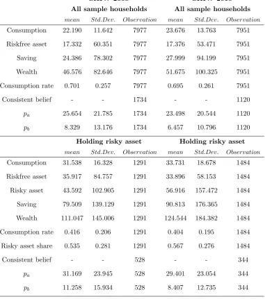
5.1 Descriptive statistics . . . 120

5.2 Distribution of recovered household belief. . . 122

5.3 OLS regression of household belief SHIW 2008 . . . 125

5.4 OLS regression of household belief SHIW 2010 . . . 126

5.5 Probit regression for market participation. . . 128

5.6 Cross-sectional test of risky asset share invariant to saving SHIW 2008 . . . 130

5.7 Cross-sectional test of risky asset share invariant to saving SHIW 2010 . . . 131

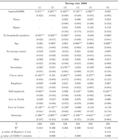
5.8 Cross-sectional test of saving rate invariant to wealth SHIW 2008 . . . 133

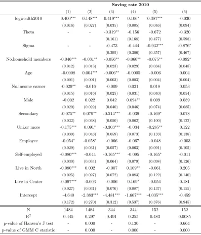
5.9 Cross-sectional test of saving rate invariant to wealth SHIW 2010 . . . 134

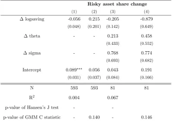
5.10 Panel test of risky asset share invariant to saving . . . 135

5.11 Panel test of saving rate invariant to wealth . . . 136

5.12 Recovered risk and ambiguity aversions based on panel data 137 5.13 Recovered risk and ambiguity aversions based on cross-sectional data . . . 139

5.14 Over-identified risk aversion based on panel data. . . 141

5.15 Over-identified risk aversion based on cross-sectional data . . 141

5.16 Correlation between risk and ambiguity aversions . . . 142

5.17 OLS regression of individual preference . . . 143

5.18 OLS regression of risky asset holding . . . 145

(6)

Acknowledgments

During my PhD study at the University of Warwick, I have benefited from

many people for their advice and help, without which the successful

com-pletion of this dissertation is not possible.

I thank my supervisors Herakles Polemarchakis and Andr´es Carvajal.

They constantly give me generous and insightful advice, and encourage me

to focus and work on my research. Whenever I get lost, it is they that lead

me back to the right track. Although Andr´es Carvajal has left Warwick

since my third year and not been my supervisor officially, he guided my research all the way through my PhD life, and his help has never stopped.

It is really a great honor for me to work with them.

I also thank Pablo Beker, Alan Bester, Ken Binmore, Valentina Corradi,

Mirko Draca, Philiph Reny, and John Stovall, whose helpful comment and

valuable feedback on my work improve the dissertation a lot.

I thank my family, especially my parents, for their love and

encourage-ment. When I feel disappointed and hopeless, their loving support helps

me pick up confidence and carry on my study.

Part of the dissertation was written while I visited the Economics De-partment at the University of Western Ontario in the academic year

2013-2014. It is pleasant and productive experience for me and their hospitality

is gratefully acknowledged.

Finally, I gratefully acknowledge the financial support from the

UK-China Scholarships for Excellence programme and from the Warwick

(7)

Declaration

This thesis is submitted to the University of Warwick in support of my

application for the degree of Doctor of Philosophy. It has been composed

by myself, except Chapter2and Chapter3, each of which has derived from

collaborative work with both Herakles Polemarchakis and Larry Selden. It

has not been submitted in any previous application for any degree.

Xinxi Song

(8)

Abstract

Preference under Ambiguity: Testing and Identification

Xinxi Song

October 2015

This dissertation focuses on testing and identifying individual ambiguity

preference under the framework of ”smooth ambiguity preference”

devel-oped by Klibanoff, Marinacci, and Mukerji (2005). Following the seminal

contributions ofAllais(1953) andEllsberg (1961), experimental data have

consistently demonstrated that individuals do not behave in accordance

with predictions of the expected utility model when they face uncertainty.

As one important class of ambiguity utility, the smooth ambiguity model

distinguishes ambiguity aversion from risk aversion, which makes the

com-parative statics possible. However, currently there is little work on testing

and recovering such preferences based on observable choices.

The dissertation contains four parts. Chapter 2uses two approaches to

derive the necessary and sufficient conditions for observed individual

port-folio choice to be compatible with the smooth ambiguity preference. The

first approach is the revealed preference method, and is based on finite

ob-servations. The second approach is demand function testing, and is based

on infinite observations. Chapter 3 establishes the conditions under which

the smooth ambiguity preference can be uniquely identified from individual

demand functions. In Chapter 4, I extend the argument of Varian (1988)

to multiple observations and incomplete market case to non-parametrically

test different shapes of risk aversion, and then to test hypotheses on shapes

of ambiguity aversion. In Chapter5, to use household survey data to

iden-tify household risk and ambiguity aversion, I build a simple parametric

model to identify household risk and ambiguity aversion from their saving

and portfolio choice. The data from the Bank of Italy Survey on Household

Income and Wealth 2008 and 2010 support the constant relative risk

aver-sion and constant relative ambiguity averaver-sion hypothesis, and give evidence

(9)

Chapter 1 Preference under ambiguity

1.1 Testing and identification

Over the past 50 years following the seminal contributions ofAllais(1953)

and Ellsberg (1961), laboratory data predominantly based on observed

choices over lotteries, have consistently demonstrated that individuals do not behave in accordance with predictions of the expected utility model.

In recent years, extensive effort has concentrated on developing models

that accommodate the fact that in many real world problems individuals

face choices characterized by uncertainty, and not just risk. This is not

handled well by expected utility maximizers who exhibit behaviour

reflect-ing the Ellsberg paradox. One class of models that focus on incorporatreflect-ing

uncertainty and overcoming the problems of the expected utility theory is

referred to as ambiguity preferences.

A number of alternative models of ambiguity preferences have been

developed. These include multiple-priors or maxmin preference, Gilboa

and Schmeidler(1989), smooth ambiguity preference,Klibanoff, Marinacci,

and Mukerji (2005), multiplier preference, Anderson, Hansen, and

Sar-gent(2003), variational preference, Maccheroni, Marinacci, and Rustichini

(2006), vector expected utility, Siniscalchi (2009). For some relevant

lit-erature on decision theory, see Etner, Jeleva, and Tallon (2012), Gilboa

(2009), and Gilboa and Marinacci (2011). The applications of

ambigu-ity preference in economic and finance modelling include portfolio choice

and asset pricing Collard, Mukerji, Sheppard, and Tallon (2011), Epstein

(10)

Miao(2012), and macroeconomicsHansen and Sargent(2001),Hansen and

Sargent (2007),Hansen, Sargent, Turmuhambetova, and Williams (2006). This dissertation focuses on the ”smooth ambiguity preference” model

due to Klibanoff, Marinacci, and Mukerji (2005). There are two reasons:

first of all, this model explicitly separates ambiguity aversion from risk

aversion, so it is meaningful to test the restrictions of ambiguity aversion,

and to identify the ambiguity aversion index; secondly, the utility function

is well-behaved, i.e. it is differentiable and concave, so the analytic

ma-chinery developed in utility and expected utility theory can be generalized

to deal with ambiguity utility.

This dissertation will address two questions: what are the testable re-strictions of the smooth ambiguity model on observable individual portfolio

choice? if an individual’s portfolio choice is compatible with the smooth

ambiguity model, could his ambiguity preference be uniquely identified?

The first question deals with existence problem, and the second deals with

uniqueness problem.

In Chapter 2, we will derive the necessary and sufficient conditions for

observed portfolio choice to be consistent with the strictly increasing, and

strictly concave smooth ambiguity preference, using two approaches:

re-vealed preference approach and demand function approach. The rere-vealed

preference approach developed byAfriat(1967) andVarian(1982) requires only finite observations of individual portfolio choice, and does not specify

any parametric utility functional form, thus is fully nonparametric. The

conditions developed here consist of nonlinear inequalities, and can be used

to test portfolio choice from incomplete markets. The demand function

ap-proach assumes individual asset demand functions are given. We develop

two tests based on demand functions: a functional form test and a demand

derivative test. The demand functional form test requires the observed

asset demands have particular functional form restrictions, while the

de-mand derivative test gives Slutsky−like restrictions. Unlike in the revealed preference test, we assume there are complete state consumption claims

contingent on both ambiguity states and risk states. Such an assumption

is extreme, and such data can be obtained only under well controlled

labo-ratory experiments. However, we think to derive theses restrictions in ideal

data case is an important first step to understanding the implications of

(11)

In Chapter 3, we assume observed individual asset demands pass the

tests in Chapter 2, and develop conditions under which his smooth ambi-guity utility function can be uniquely identified. In Chapter 2, the smooth

ambiguity preference can be explicitly constructed if an individual’s asset

demands satisfy the revealed preference conditions; however, such

construc-tion is not unique, since finite observaconstruc-tions cannot pin down an individual’s

indifference curves. We tackle uniqueness by assuming individual asset

de-mand functions given. This work builds on the recoverability literature for

expected utility preferences in Green, Lau, and Polemarchakis (1979) and

Dybvig and Polemarchakis (1981). For us to address the recoverability of

ambiguity preferences, several important new technical results are required. We assume there is one riskless asset and one ambiguity-free asset (i.e. the

payoff distribution is invariant across ambiguity states). We show that

un-der these assumptions and one technical condition (full rank condition),

the individual’s risk aversion index and ambiguity aversion index can be

uniquely identified from his asset demand functions. The technical

condi-tion basically means individual has ambiguity on the mean return of risky

assets. The existence of riskless and ambiguity free asset can be relaxed;

however, it will put more restrictions on the underlying utility function,

like time separability and analyticity at 0.

Chapter 4tests the restrictions of smooth ambiguity preference with a particular shape (decreasing or increasing ambiguity aversion) on

portfo-lio choice, and gives lower and upper bounds for these measures. Recent

papers in economics and finance show that the implication of the smooth

ambiguity model crucially depends on the shape of the risk and ambiguity

aversion and their magnitudes. Varian (1988) derives the nonparametric

restrictions of decreasing or increasing absolute (increasing) risk aversion

on one observation of Arrow−Debreu security, and gives the lower and up-per bounds for these measures. I revisit Varian’s argument, and extend it

to multiple observations in incomplete markets. The conditions involve the existence of Afriat numbers, and can be used to bound risk aversion. Then

the restrictions of different shapes of ambiguity aversion are derived.

Chapter 5 investigates systematically the nature of household

ambigu-ity preferences using household survey data within a parametric framework.

Despite the importance of individual risk aversion and ambiguity aversion

(12)

there is rare evidence on the shape of individual ambiguity preferences,

except a little evidence from either lab experiments or pure thought ex-periments using variants of Ellsberg’s urns. I derive an explicit solution

in a two-period smooth ambiguity model due to Klibanoff, Marinacci, and

Mukerji(2005) assuming constant relative risk aversion and constant

rela-tive ambiguity aversion, and show that time preference, risk aversion and

ambiguity aversion can be uniquely identified from a special panel dataset.

From the Bank of Italy Survey on Household Income and Wealth (SHIW)

2008 and 2010, the most important findings are: constant relative risk

aversion and relative ambiguity aversion can be a good approximation; the

recovered preference parameters display considerable heterogeneity; the av-erage relative risk aversion is much smaller than 1; and the avav-erage

rela-tive ambiguity aversion is around 3 or larger. Other interesting findings

include, firstly, households’ expectations are very pessimistic, and are

sub-ject to much ambiguity; secondly, the over-identification restriction implied

by the subjective expected utility model rejects the null hypothesis that

households are subjective expected utility maximizers, in favor of the

am-biguity model; finally, household risk aversion and amam-biguity aversion are

not correlated, can’t be explained by observable household characteristics,

and have a quantitatively significant effect on consumption and portfolio

holding.

This dissertation contributes to understanding smooth ambiguity

pref-erence both theoretically and empirically. Chapters 2-4provide theoretical

foundation for future empirical work on testing and recovering individual

smooth ambiguity preference. Chapter5 provides fresh empirical evidence

on the shape and magnitude of household risk and ambiguity aversion based

on household consumption and saving data, which sheds light on the

dis-tribution of ambiguity preference, and can be used in finance and

macroe-conomic calibration to examine the implication of ambiguity preference

models.

In the next section of this chapter, I set up the economic environment

in which a consumer makes his choice. This model setup and notations will

(13)

1.2 Setup

In this dissertation, I consider a one-good two-period economy. Assume

states of the world in the second period are represented by ω∈Ω, a finite set that has a product structure: Ω =A × S, where a ∈ A are states of uncertainty while s ∈ S are states of risk.1 _Ω _{can be interpreted as the}

set of possible outcomes of two-stage lotteries, whereA includes outcomes

of the first stage lotteries, and S includes realizations of the second stage

lotteries. I follow the literature, and assume that the consumption and

the payoff of financial assets are contingent on the realization of risk states only.2 _{For a finite set} _E_{, let} _∆_E _{be the set of probability measures on} _E_,

or, equivalently, the simplex of dimension (#E−1). A probability measure on the set of the states of the world isπ ∈∆(Ω), and it decomposes

π = (µ⊗ν)

into a probability measure over states of the uncertainty

µ∈∆(A)

, and a family of conditional probability measures over states of risk

νa:A→∆(S);

evidently,

π(a, s) =µ(a)ν(s|a).

From now on, for notational ease, I denote π(a, s) by πas, µ(a) by µa,

and ν(s|a) by νas.

A distribution of wealth across the risk states is

x= (..., xs, ...)∈ ×s(0,∞).

1_{The exception is Chapter}₅_{, where I assume lognormal distribution with a continuum} of states.

2_{If consumption and asset payoff depend on both uncertainty and risk states, as}

(14)

A utility function over distribution of wealth is

U :×s(0,∞)→R.

It is continuous, strictly monotonically increasing and strictly quasi−concave. In the interior of its domain of definition, DU 0, and D2U is negative definite on the orthogonal complement of the gradient, DU⊥.

Savage (1954) or, alternatively, Anscombe and Aumann (1963) derive

a probability measure

π =µ⊗ν

, and a cardinal risk−uncertainty index

u: (0,∞)→_R,

such that

U(x) = Eπu(xs) =EµEνau(xs).

3 _(1.1)

Gilboa and Schmeidler (1989) derive a convex set of probability mea-sures

C ⊂∆(Ω)

and a risk index

u: (0,∞)→_R,

such that

U(x) = min

π∈CEπu(xs). (1.2)

Klibanoff, Marinacci, and Mukerji (2005) derive a probability measure

π =µ⊗ν,

and a (cardinal) risk index and an uncertainty index

u: (0,∞)→_R and ˜φ:u((0,∞))→_R,

3_{In the original formulation in} _Savage ₍₁₉₅₄_{), the domain of preference does not}

(15)

respectively, such that

U(x) =Eµφ E˜ νau(xs)

.

Alternatively,

φ : (0,∞)→_R

and

U(x) = Eµφ

u−1 Eνau(xs)

, (1.3)

which, as in Selden and Wei (2014), also Hayashi and Miao (2011),

al-lows for invariance to an increasing affine transformation of the risk index

and generate appropriate comparative statics. The individual is ambigu-ity averse if φ is a concave transformation of u, and ambiguity neutral if

φ◦u−1 _{is linear. Evidently,} _φ _{= ˜}_φ_◦_u _{establishes the equivalence of the}

formulations.

Within the framework of Anscombe and Aumann (1963),µis the

sub-jective probability over horse race lotteries, and ν is the objective

proba-bility over roulette wheels. As shown by experimental evidence in Halevy

(2007), the non-reduction of compound objective lotteries is also

consis-tent with the smooth ambiguity aversion, in which case both µ and ν are

objective probabilities.

More generally, individual ambiguity preference can be defined without

reference to the probability of ambiguity states:

U(x) = Φ w(x)

= Φ ..., wa(x), ...

, (1.4)

where

wa(x) = u−1(Eνau(xs)),

is the certainty equivalent wealth at a state of uncertainty, a;

ν :A→∆(S),

is a family of conditional probability measures over states of risk;

(16)

the distribution of certainty equivalent wealth across states of uncertainty;

u: (0,∞)→_R

is a risk index; and

Φ :×a(0,∞)→R

is an ordinal utility function over the distribution of certainty equivalent

wealth across states of uncertainty.

Evidently, others are special cases. And, there is no explicit reference to a probability measure over states of uncertainty.

There are J assets, whereJ is a finite number. Payoffs of asset j are

rj = (..., rsj, ...)

0

,

a column vector withSrows, i.e. its payoff is risk state contingent. Without loss of generality, let

Eπrj = 1.

At a state of risk, payoffs of assets are

Rs = (..., rsj, ...),

a row vector with J columns. The matrix of asset payoffs is

R= (...,rj, ...) = (...,Rs, ...),

a matrix of full column rank.

A portfolio of assets is

y= (..., yj, ...).

It generates the distribution of wealth across states of risk

x=Ry.

(17)

of wealth across states of risk is non-empty,

Y ={y:Ry 0} 6=∅;

since R is of full column rank, Y is open. The domain of prices of assets

that do not allow for arbitrage is

(18)

Chapter 2 Testing smooth ambiguity

preference

2.1 Introduction

The standard consumer theory assumes that a rational consumer will

max-imize his well-behaved utility function subject to a budget constraint. In

certainty case, the testable implications of such theory have been derived

from two different approaches. The first approach dated back to Antonelli

(1971) and Slutsky (1960) is to assume the whole demand function is

ob-servable, and derives the necessary and sufficient condition on the derivative

of demand functions, which is known as Slutsky equation.1 The second

ap-proach attributed to Samuelson(1938), Afriat (1967),Diewert (1973) and

Varian(1982) is to assume finite data observation, and derive the necessary and sufficient condition to be compatible with utility maximization, which

is known as Afriat theorem, see Kreps (2013).2

Under risk, a rational consumer’s preference is expressed as expected

utility invon Neumann and Morgenstern(1944),Savage(1954) andAnscombe

and Aumann (1963). The testable restrictions of expected utility theory

1_{For the Slutsky condition to be sufficient, income-Lipschitz condition of the demand}

functions-i.e. the derivative of the demand functions with respect to income is bounded on the domain, is needed, seeHurwicz and Uzawa(1971).

2_{This approach is called revealed preference approach since originally the conditions}

(19)

have been exploited using both approaches. Kubler, Selden, and Wei(2014)

derive Slutsky conditions under complete markets, which involves deriva-tives of demand function with respect to probability. Basically, they work

in the framework of von Neumann and Morgenstern (1944), and they

as-sume probability is observable and changes across observations. They also

give a functional form test, where the contingent claim demand must

sat-isfy certain form restrictions. Polemarchakis and Selden (1983) derive the

Slutsky-like conditions under incomplete markets, where the probability

is fixed, and the conditions involve the existence of some unknown

func-tions. The revealed preference conditions have been developed by Green

and Srivastava (1986), and Kubler, Selden, and Wei (2014). The model setup in Green and Srivastava (1986) is quite general, and is applicable

to incomplete markets, and multiple goods in each state. The necessary

and sufficient conditions there involve existence of unknown utility levels

and multipliers. Kubler, Selden, and Wei (2014) assume one good in each

state under complete markets, and characterize the necessary and sufficient

conditions by strong axiom of revealed expected utility (SAREU), which is

free of existential quantifiers.

The expected utility theory has been challenged by Ellsberg’s paradox

Ellsberg (1961) and other experimental evidence, which demonstrate that

individual’s choice will violate the independence axiom when he is am-biguous about the probability distribution of relevant events.3 _{In recent}

years, the decision theory literature has developed alternative models to

accommodate individual choice behavior under ambiguity. In developing

laboratory tests of whether a particular model provides a satisfactory

de-scription of choices of individuals, decision theorists have focused on choices

over lotteries whereas the economists alternatively have focused on choices

over assets (or contingent claims). One potentially important limitation of

the former is that the choices over lotteries reflect neither variable prices for

lotteries nor budget constraints associated with a fixed income. In recent work that overcomes the latter problem, there has been considerable focus

on developing revealed preference tests, where following the classic work of

Afriat(1967) andVarian(1982), one seeks to verify whether observed asset

(price,quantity) pairs are consistent with specific demand tests derived for

(20)

assumed non-parametric forms of utility (such as additive separability or

weak separability). Two important applications of this approach to ambi-guity preferences are Bayer, Bose, Polisson, and Renou (2013) and Ahn,

Choi, Gale, and Kariv (2014). For instance in the former, the authors

de-rive testable inequality conditions, associated with the assumed risk and

ambiguity indices, which are consistent with maximization of ambiguity

preferences. This work, while extremely interesting, would seem to have

two limitations. First, only very special non-parametric forms of ambiguity

preferences can be addressed. Second, almost all of the revealed preference

work in risky or uncertain settings of which we are aware makes the very

strong assumption of complete asset markets where the number of states of nature equals the number of assets, which span the state space.

In this chapter, we use both revealed preference approach and demand

function approach to test smooth ambiguity model. In both approaches, we

assume the probability distributions are known, and change across

obser-vations.4 _{The revealed preference approach does not put any requirement}

on the financial market, i.e. the necessary and sufficient conditions can be

used to test portfolio choice from incomplete markets. For demand function

tests, we assume complete state consumption contingent on both ambiguity

and risk states.

2.2 Revealed preference test

As mentioned in Section1.2in Chapter 1, the ambiguity preference can be

written more generally as

U(x) = Φ

..., Eνau(xa), ...

. (2.1)

We will put some regularity assumptions on the functional form (2.1)

and asset return structure to make the individual optimization problem

well-defined.

Assumption 1

(1) u isC2 on _R++, is strictly concave and satisfies ∀x∈R++,u

0

>0;

4_{As will be seen, observing the probability distribution is not necessary for the}

(21)

(2) Φ is C1 on _RA₊₊, is strictly concave, and satisfies ∀w(x) ∈ _RA

++,

Φa>0 for all a= 1, ..., A;

(3) Φ ..., u−1₍_E

νau(xs)), ...

is strictly quasi-concave on _RS

++.

Assumption 2 For each conditional probability distribution va, the

gross return rj of asset j,j = 1, ..., J satisfies:

(1) prob{rj ≥0} =1;

(2) prob{rj = 0} 6= 1;

(3) rj is linearly independent with return vectors of other assets;

(4) Eνar

l

j <+∞.

Now we specify the data we can observe: dataD={pn_,_yn_,_νn a,R}

n=1,...,N a=1,...,A.

So the dataDincludeN observations of asset pricesp, portfolio choices

y, all conditional probability distributionsv, and the asset payoff structure

R, which satisfies Assumption 2.

Remark 1. No matter the domain of preference is subjective-objective

two-stage lotteries as inAnscombe and Aumann(1963) or a compoundobjective

lotteries as shown by Halevy (2007), the conditional distributions are

ob-jective. So assuming observation of conditional probability distribution

seems to be a tenable assumption. In the experiments ofEllsberg (1961) or

other experiments like Ahn, Choi, Gale, and Kariv (2014), the conditional

probabilities are objectively known to the subjects.

To test the ambiguity preference (2.1) based on finite observations in

dataset D, we extend the revealed preference method developed byAfriat

(1967), Varian (1982) and Matzkin and Richter (1991) to our setting.

Proposition 1 presents the necessary and sufficient conditions for finite

observations in datasetDto be consistent with such ambiguity preference.

Proposition 1. The following conditions are equivalent:

(i) There exists a continuous, locally non-satiated utility function

U(y) = Φ ...,

S

X

s=1

νasu J

X

j=1

rsjyj

!

, ...

!

(22)

where Φ and u satisfy Assumption 1, to rationalize the data D, i.e. for all n= 1, ..., N

yn ∈arg max

y∈_RJ

U(y) s.t. pn·y≤pn·yn.

(ii) There exist real numbers(Un s, Msn)

n=1,...,N

s=1,...,S >0,(Φn) N

n=1,(ρna)

n=1,...,N a=1,...,A >

0, and (λn)N_n₌₁ > 0 such that for all n, m ∈ {1,2, ..., N}, s, s0 ∈ {1,2, ..., S}, a, a0 ∈ {1,2, ..., A} and j ∈ {j = 1,2, ..., J} 5

U_sn−U_sm0 < M_sm0

J

X

j=1

rsjyjn− J

X

j=1

rs0_jym

j

!

,

with equality if PJ

j=1rsjynj =

PJ

j=1rs0_jy_jm; Φn−Φm <

A

X

a=1

ρm_a

S

X

s=1

ν_asnU_sn− S

X

s=1

ν_am0_sU_sm !

,

with equality if PS

s=1ν

n asUsn=

PS

s=1ν

m a0_sU_sm;

and

A

X

a=1

ρn_a

S

X

s=1

ν_asnM_snrsj

!

=λnpn_j.

Proof. (i) implies (ii)

The first order conditions are∀j ∈ {1,2, ..., J},

A

X

a=1

Φ0_a ...,

S

X

s=1

ν_asnu

J

X

j=1

rsjynj

!

, ...

! X

s

ν_asnu0

J

X

j=1

rsjyjn

!

rsj

!

=λpn_j.

(2.2)

Since u and Φ are both strictly concave, the following inequalities hold

u

J

X

j=1

rsjyjn

!

< u

J

X

j=1

r_s0

jy m j

!

+u0

J

X

j=1

r_s0

jy m j

! _J X

j=1

rsjyjn− J

X

j=1

rs0_jym_j !

,

(2.3)

5_{In this condition, the numbers (}_Un s)

n=1,...,N

(23)

and

Φ ...,

S

X

s=1

ν_asnu

J

X

j=1

rsjyjn

!

, ...

!

<Φ ...,

S

X

s=1

ν_asmu

J

X

j=1

rsjyjm

! , ... ! + A X a=1

Φ0 ...,

S

X

s=1

ν_asmu

J

X

j=1

rsjyjm

! , ... ! × S X s=1

ν_asnu

J

X

j=1

rsjyjn

!

− S

X

s=1

ν_am0_su

J

X

j=1

rsjyjm

!!

. (2.4)

Denoting

U_sn =u

J

X

j=1

rsjyjn

!

, M_sn =u0

J

X

j=1

rsjyjn

!

,

Φn = Φ ...,

S

X

s=1

ν_asnu

J

X

j=1

rsjynj

!

, ...

!

,

ρn_a = Φ0_a ...,

S

X

s=1

ν_asnu

J

X

j=1

rsjyjn

!

, ...

!

.

The conditions (2.2), (2.3), and (2.4) can be rewritten as

J

X

j=1

rsjyjn− J

X

j=1

rs0_jym

j

!

, (2.5)

Φn−Φm <

A

X

a=1

ρm_a

S

X

s=1

ν_asnU_sn− S

X

s=1

ν_am0_sU_sm ! , (2.6) and A X a=1

ρn_a

S

X

s=1

ν_asnM_snrsj

!

=λnpn_j. (2.7)

(ii) implies (i)

Given the solution to inequalities in (ii), i.e. real numbers (U_sn, M_sn)n_s₌₁=1_,...,S,...,N >

0, (Φn)N_n₌₁, (ρn_a)n_a₌₁=1_,...,A,...,N >0 and (λn)N_n₌₁ >0, we will modify the argument inMatzkin and Richter (1991) to construct strictly increasing and strictly

(24)

Step 1: construction of u(x)

Since we have only finite inequalities, we can choose small enough

num-ber δ0 such that

J

X

j=1

rsjyjn− J

X

j=1

rs0_jym

j

!

−δ0, (2.8)

for PJ

j=1rsjy

n j 6=

PJ

j=1rs0jy

m j .

Define a function g :_R1 _→

R1 by

g(x) = (x2+T)12 −T 1

2, (2.9)

where T is a positive real number.

It can be shown that the defined function g(x) is nonnegative valued, differentiable, strictly convex, and has bounded derivative. And condition

(2.8) implies that we can choose a small enough number δ such that

J

X

j=1

rsjyjn− J

X

j=1

rs0_jy_jm !

−δg

J

X

j=1

rsjyjn− J

X

j=1

rs0_jy_jm !

,

(2.10)

for PJ

j=1rsjy

n j 6=

PJ

j=1rs0jy

m j .

Define functions un

s(x) :R1 →R1 by

un_s(x) =U_sn+M_sn x− J

X

j=1

rsjynj

!

−δg x− J

X

j=1

rsjyjn

!

, (2.11)

where n∈ {1,2, ..., N}, s∈ {1,2, ..., S}.

It can be shown that the defined functionun

s(x) is strictly concave, and

satisfies un s

PJ

j=1rsjyjn

=Un s.

(25)

u(x) = min

s,n {u n

s(x)}. (2.12)

The defined function u(x) is strictly concave, and we can choose δsmall enough that the function u(x) is strictly increasing. This is possible since the defined function g(x) has bounded derivative and there are finite in-equalities.

We claim that u(PJ

j=1rsjyjn) =Usn,since

u

J

X

j=1

rsjyjn

!

=um_s0

J

X

j=1

rsjyjn

!

≤un_s

J

X

j=1

rsjyjn

!

=U_sn (2.13)

The inequality in above equation can not be strict, otherwise it will

violate inequality (2.10).

Step 2: construction of index Φ(u):

We will sketch the construction, since it follows the same argument as

above.

Define a function G(u) :_RA_→ R1 by

G(u) = (u2₁+...u2_A+T)12 −T 1

2. (2.14)

Choose small enough positive real number such that

Φn−Φm <

A

X

a=1

ρm_a

S

X

s=1

ν_asnU_sn− S

X

s=1

ν_am0_sU_sm !

−G ...,

S

X

s=1

ν_asnU_sn− S

X

s=1

ν_am0_sU_sm, ... !

, (2.15)

for PS

s=1ν

n asUsn 6=

PS

s=1ν

(26)

Define functions φn(u) :_RA→_R1 _by

φn(u) = Φn+

A

X

a=1

ρm_a ua− S

X

s=1

ν_am0_sU_sm !

−G ..., ua− S

X

s=1

ν_am0_sU_sm, ... !

,

(2.16)

where n∈ {1,2, ..., N}, a∈ {1,2, ..., A}.

It can be shown that the defined function φn(u) is strictly concave and satisfies φn

...,PS

s=1ν

n asUsn, ...

= Φn.

Define a function Φ : _RA_→ R1 by

Φ(u) = min

n {φ

n₍_u₎_}_. _(2.17)

The defined function Φ(u) is strictly concave, and we can choose

small enough such that Φ(u) is strictly increasing. It can be shown that

Φ...,PS

s=1νasnUsn, ...

= Φn_.

Step 3: rationalization

We claim that the constructed utility function rationalizes the observed

data, i.e. if pi_yi _>_pi_y _and _yi ₆₌_y_{, then}

Φ ...,

S

X

s=1

ν_asi u

J

X

j=1

rsjyji

!

, ...

!

>Φ ...,

S

X

s=1

ν_asi u

J

X

j=1

rsjyj

!

, ...

!

.

(27)

Φ ...,

S

X

s=1

ν_asi u

J

X

j=1

rsjyj

! , ... ! 1 = min m

Φm+

A

X

a=1

ρm_a

S

X

s=1

ν_asi u

J

X

j=1

rsjyj

− S

X

s

ν_am0

sU m s −G ..., S X s=1

ν_asi u

J

X

j=1

rsjyj

− S

X

s

ν_a0

sU m s , ...

2 = min

m

Φm+

A

X

a=1

ρm_a

S

X

s=1

ν_asi min

s0,n

U_sn0 +Mn

s0 J

X

j=1

rsjyj− J

X

j=1

r_s0

jy n j −δg J X j=1

rsjyj − J

X

j=1

r_s0

jy n j − S X s

ν_am0

sU m s −G ..., S X s=1

ν_asi u

J

X

j=1

rsjyj

− S

X

s

ν_am0

sU m s , ...

3

≤ Φi+

A

X

a=1

ρi_a

S

X

s=1

ν_asi U_si+M_si

J

X

j=1

rsjyj− J

X

j=1

rsjyji

−δg

J

X

j=1

rsjyj − J

X

j=1

rsjyij

− S

X

s

νasUsi

−G ..., S X s=1

νasu J

X

j=1

rsjyj

− S

X

s

ν_asi U_si, ...

4

< Φi+

A

X

a=1

ρi_a

S

X

s=1

ν_asi U_si+M_si

J

X

j=1

rsjyj− J

X

j=1

rsjyji

− S

X

s

ν_asi U_si

= Φi+

A

X

a=1

ρi_a

S

X

s=1

ν_asi M_si

J

X

j=1

rsjyj − J

X

j=1

rsjyij

5

= Φi+λipi(y−yi) 6

≤ Φi

7 = Φ ..., S X s=1

ν_asi U_si, ...

8 = Φ ..., S X s=1

ν_asi u

J

X

j=1

rsjyij

, ...

(28)

where 1 follows from the definition of function Φ, 2 from the definition

of function u, 3 from taking the minimum, 4 from positivity of functions

g and G, 5 from equation (2.7), and 6 from the budget constraint.

Remark 2. As inMatzkin and Richter(1991), we can prove the constructed

function is generically infinitely differentiable. And if we put further

re-strictions: M_sn = M_sm0 if PJ

j=1rsjy

n j =

PJ

j=1rs0jy

m

j , and ρna = ρma0 if PS

s=1ν

n asUsn =

PS

s=1ν

m

a0_sU_sm, then we can use the convolution methods in

Chiappori and Rochet (1987) to smooth our defined functions to be

in-finitely differentiable on the whole domain. So with finite observations,

differentiability is not testable, in the first statement the differentiability

of the objective function is not needed.

Remark 3. In the above testing, we assume the conditional probability is

observed, and varies across observations. The assumption of observing

con-ditional probability can be relaxed, in stead, we can require the existence

of these numbers in condition (ii); however, in this case, we need to assume

these probabilities are fixed across observations, otherwise the testability

will be lost.

The smooth ambiguity model of Klibanoff, Marinacci, and Mukerji

(2005) is a special case when

Φ(..., Eνau(xs), ...) =

A

X

a=1

µaφ S

X

s=1

νasu(xs)

!

. (2.19)

Here the probability of ambiguity states is explicitly referred to. We

put the following restrictions on the functional form (2.19).

Assumption 10

0

>0;

(2) φ is C2 on _R++, is strictly concave, and satisfies ∀w(x) ∈ R++,

φ0 >0;

(3) φ u−1(.) is strictly concave on _R.

To test this functional form, we specify the following data set.

Data D0={pn_,_yn_,_µn_,_νn a,R}

(29)

So the data D0 includes N observations of asset prices p, portfolio choices y, the probability distribution over ambiguity states µ, all condi-tional probability distributions v, and the asset payoff structure R, which

satisfies Assumption 2.

Remark 4. We assume the observation of both µ, the probability over

ambiguity states, and ν, the conditional probability over risk states. If

the domain of preference is compoundobjective lotteries, such assumption

seems to be reasonable. Within the framework of Anscombe and Aumann

(1963), it seems much less plausible to observe probability µ. In the

fol-lowing corollary, we state the necessary and sufficient conditions assuming

observation of µ; however, as pointed out in remark 3, we can require the

existence of these numbers when they are not observable.

Corollary 1 gives the corresponding necessary and sufficient conditions

for data D0 to be consistent with this particular functional form.

Corollary 1. The following conditions are equivalent:

(i) There exists a continuous, locally non-satiated utility function

U(y) =

A

X

a=1

µaφ S

X

s=1

νasu J

X

j=1

rsjyj

!!

,

where φ and u satisfy Assumption 10, to rationalize the data D0, i.e. for all i= 1, ..., N

yn ∈arg max

y∈RJ

U(y) s.t. pn·y≤pn·yn.

(ii) There exist real numbers(U_sn, M_sn)_sn₌₁=1_,...,S,...,N >0,(Φ_an)n_a₌₁=1_,...,A,...,N,(ρn_h)n_a₌₁=1_,...,A,...,N >

0 and (λn₎N

n=1 > 0 such that for all n, m ∈ {1,2, ..., N}, s, s

0 _∈

{1,2, ..., S}, a, a0 ∈ {1,2, ..., A} and j ∈ {j = 1,2, ..., J}

J

X

j=1

rsjyjn− J

X

j=1

rs0_jym

j

!

(30)

with equality if PJ

j=1rsjynj =

PJ

j=1rs0_jy_jm; Φn_a −Φm_a0 < ρm_a0

S

X

s=1

ν_asnU_sn− S

X

s=1

ν_am0_sU_sm !

,

with equality if PS

s=1ν

n asUsn=

PS

s=1ν

m

a0_sU_sm; and

A

X

a=1

µn_aρn_a

S

X

s=1

ν_asnM_snrsj

!

=λnpn_j.

Proof. We can modify the proof of Proposition 1 to prove this result. To

prove (i) implies (ii), use the strict concavity of function u, the strict con-cavity of functionφ, and the first order condition. To prove (ii) implies (i), the construction of u(x) follows the same argument. We give a sketch of the construction of φ(u).

Construction of index φ(u):

Choose a small enough positive real number such that:

Φn_a−Φm_a0 < ρm_a0

S

X

s=1

ν_asnU_sn− S

X

s=1

ν_am0_sU_sm !

−g

S

X

s=1

ν_asnU_sn− S

X

s=1

ν_am0_sU_sm !

,

(2.20)

for PS

s=1νasnUsn 6=

PS

s=1νam0_sU_sm.

Define functions φn_a(u) :_R1 →_R1 _by

φn_a(u) = Φn_a +ρn_a u− S

X

s=1

ν_asnU_sn

!

−g u− S

X

s=1

ν_asnU_sn

!

, (2.21)

where n∈ {1,2, ..., N}, a∈ {1,2, ..., A}.

It can be shown that the defined function φn

a(u) is strictly concave and

satisfies φn a

PS

s=1νasnUsn

= Φn a.

(31)

φ(u) = min

a,n {φ n

a(u)}. (2.22)

The defined function φ(u) is strictly concave, and we can choose

small enough such that φ(u) is strictly increasing. It can be shown that

φPS

s=1ν

n asUsn

= Φn a.

We omit the remaining details of rationalization.

Remark 5. Bayer, Bose, Polisson, and Renou (2013) is a complete market

version of Corollary1, so a special case of Proposition1, and our conditions

can test observations from incomplete markets. Our conditions are stated

for strictly concave functions, but if the strict inequalities are changed to be

weak inequalities, they will become necessary and sufficient conditions for

testing weakly concave smooth ambiguity utility under incomplete markets.

2.3 Demand function tests

In the following demand function tests, we deviate from the literature, and

assume that both probability of ambiguity and probability of risk are

ob-servable, and contingent consumption can be traded contingent on both

states. If the domain of preference is compound objective lotteries, then

such assumption is tenable. As shown by experimental evidence in Halevy

(2007), the non-reduction of compound objective lotteries is also

consis-tent with the smooth ambiguity aversion, in which case both µ and ν are

objective probabilities. If the domain of preference is horse race-roulette wheel two-stage lotteries, the the first stage subjective probability should

be elicited from subjects.

For both demand function tests, we assume the probabilities µ and

ν change across observations. When consumers can trade consumption

claims contingent on both ambiguity and risk states, their utility function

is defined over distribution of consumption over states of the world:

U(x;µ;ν) =Eµφ

Eνau(xas)

.6 (2.23)

6_{That probabilities}_µ_and_ν_{enter the objective function means probabilities change}

(32)

We are interested in consumers who are both risk and ambiguity averse,

and put the following regularity restrictions on the function (2.23):

Regularity Assumption 100

0

>0;

(2) φ is C2 on_R, is strictly concave, and satisfies ∀x∈_R, φ0 >0. Because both of our demand function tests crucially depend on

separa-bility of the objective function, we first give the concepts of separasepara-bility we

use. Forncommodities, the set of these commodities is denoted byN, i.e.

N = {1, ..., n}. A partition of the set N is a class of mutually exclusive and exhaustive subsets {N1, ...,NT} such that N =N1∪...∪NT, and

Ns∩Nt =∅ for s =6 t. So a commodity bundle x = (x1, ..., xn) is

corre-spondingly partitioned into (x(1), ...,x(T)), where for each t, the sub-vector

x(t) _{is composed of} _x

i, i∈Nt.

Definition 1. A utility function u(x) is strongly separable with respect to partition{N1, ...,NT}withT >2, ifu(x) =u(x(1), ...,x(T)) is of the form

u(x) =F u1(x(1)) +...+uT(x(T)), (2.24) where F(y) is a monotone-increasing function of one variable y, and for each t= 1, ..., T, ut(x(t)) is a function of sub-vector x(t).

Definition 2. A utility function u(x) is weakly separable with respect to partition{N1, ...,NT}withT >2, ifu(x) =u(x(1), ...,x(T)) is of the form

u(x) = _z u1(x(1)), ..., uT(x(T)), (2.25) where _z(u1, ..., uT) is a function of T variables, and for each t = 1, ..., T,

ut(x(t)) is a function of subvector x(t) alone.

Remark 6. Both definitions followGoldman and Uzawa(1964). However, in

Goldman and Uzawa(1964), their primitive definition ofstrong separability

is ∂ui(x)/uj(x)

∂xk = 0, for all i ∈ Ns, j ∈ Nt, and k /∈ Ns∪Nt (s 6= t), and that of weak separability is ∂ui(x)/uj(x)

∂xk = 0, for all i, j ∈ Nt, and k /∈ Nt.

Goldman and Uzawa (1964) prove that their primitive definitions imply

the functional forms in Definition 1 and Definition 2, respectively.

(33)

Remark 7. The concepts of both strong and weak separability are ordinal,

and a strongly separable utility function is also weakly separable.

Under the assumption of complete contingent consumption, consumer’s

objective function (2.23) satisfies the property of strong separability across

both ambiguity states and risk states. Consumer’s optimization problem is

max

x∈_RAS ++

A

X

a=1

µaφ S

X

s=1

νasu(xas)

!

, s.t. p·x≤I. (2.26)

Under the regularity assumption, solution to the problem (2.26) exists

and is unique. We assume the optimal consumption demands x(p;I;µ;ν) are observable. We want to know what properties these demand functions

possess if they are generated from problem (2.26).

2.3.1 Functional form test

Goldman and Uzawa (1964) give the conditions characterized by Slutsky terms for the observed demand functions to be consistent with a strongly

(weakly) separable utility function. Here we assume the contingent demand

functions satisfy the conditions for weak separability, the question we ask

is: when will a weakly separable utility function be of the particular form

(2.23)? Proposition 2 below gives the necessary and sufficient conditions

for the derived contingent demands to be compatible with this particular

functional form.

Proposition 2. Assume A > 2 and S > 2, and there exist complete con-tingent claims, which can be rationalized by a well-defined, weakly separable

utility. Then this utility function is ordinally equivalent to a smooth

ambi-guity utility if and only if there exist strictly monotone functionsf :_R2 ++ →

R++, γ : R++ → R++, and G : R2 → R such that for a ∈ {1, ..., A} and

s∈ {1, ..., S}, the observed contingent demands satisfy

xas =f(xa1, kas), (2.27)

S

X

s=1

νas

Z

γ(xa1)

f−1

xa1(xas)

dxas=G S

X

s=1

ν1s

Z

γ(x11)

f−1

x11(x1s)

dx1s, Ka

!

(34)

where kas =def _ννas_a₁p_pa_as1, and Ka =def

µaνa1γ(xa1)p11

µ1ν11γ(x11)pa1. And functions f and G

satisfy: x=f(x,1), u(x) =G u(x),1, and _∂x∂2G

asxa1 = 0.

Remark 8. Condition (2.27) holds for each risk state s, conditional on ambiguity state a. So it is a restriction on the relation between risk state consumption demand xas and its relative risk neutral price kas.

Remark 9. Condition (2.28) relates the expected utility in state a (ex-pressed in terms of integration of demands) to its relative ambiguity neutral

price Ka. The expected utility level depends on the absolute level of the

utility indexu, as indicated byγ function; however, the relative ambiguity neutral price is independent of the unit of u.

Lemma 1. WhenS > 2, a twice continuously differentiable utility function is additively separable u(x) = PS

s=1us(xs) if and only if ∂us/u1

∂ui = 0 for

i, s∈ {2,3, ..., S},and i6=s.

This lemma is used in Kubler, Selden, and Wei (2014), who contribute it toSamuelson(1947). However, it should be noted that we only focus on

the case of one good per state, theadditively separability is a special case of

strong separability in Definition 1, and the proof can be found in Goldman

and Uzawa (1964). Now we go to the proof of Proposition 2.

Proof. Necessity

Since the objective function (2.23) satisfies the regularity assumption,

the following first order conditions are necessary and sufficient for

charac-tering the optimal solution to problem (2.26):

F.O.C with respect to xas,

µaφ

0

S

X

s=1

νasu(xas)

!

νasu

0

(xas) =λpas, (2.29)

F.O.C with respect to x_as0,

µaφ

0

S

X

s=1

νasu(xas)

!

ν_as0u 0

(x_as0) = λp

as0, (2.30)

F.O.C with respect to x_a0

(35)

µ_a0φ 0

S

X

s=1

ν_a0

su(xa0s)

!

ν_a0

su

0 (x_a0

s) = λpa0s, (2.31)

where λ is the Lagrange multiplier.

From equations (2.29) and (2.30), we have

νasu

0 (xas)

ν_as0u0(x

as0)

= pas

p_as0

. (2.32)

From equations (2.29) and (2.31), we have

µaφ

0 _S

P

s=1

νasu(xas)

νasu

0 (xas)

µ_a0φ0 _S

P

s=1

ν_a0

su(xa0s)

ν_a0

su

0 (x_a0

s)

= pas

p_a0

s

. (2.33)

Equation (2.32) characterizes the marginal rate of substitution between

consumptions within the same ambiguity state, and equation (2.33) char-acterizes the marginal rate of substitution between consumptions across

ambiguity states.

Rearrange terms in equation (2.32), we have

u0(xas) =

νa1pas

νaspa1

u0(xa1). (2.34)

Define kas= ν_νas_a₁p_pa_as1, and substitute into equation (2.34), we have

xas =u

0₋₁u 0

(xa1)

kas

=f(xa1, kas). (2.35)

Monotonicity of functionf follows from concavity ofu(or monotonicity of u0). Note that this functional form holds contingent on each ambiguity states; however, the function f itself is invariant across ambiguity states.

To derive equation (2.28), define u0(x) = γ(x), then concavity of u

implies that γ(x) is a decreasing function ofx. From equations (2.34) and (2.35), we have

u(xas) =

Z _γ₍_x

a1)

f−1

xa1(xas)

dxas. (2.36)

(36)

φ0

S

X

s=1

νasu(xas)

!

= µ1ν1su 0

(x1s)pas

µaνasu

0

(xas)p1s

φ0

S

X

s=1

ν1su(x1s)

!

. (2.37)

Use the relation in equation (2.34), and substitute u0(x1s) and u

0 (xas)

into above equation (2.37), we have

φ0

S

X

s=1

νasu(xas)

!

= µ1ν11γ(x11)pa1

µaνa1γ(xa1)p11

φ0

S

X

s=1

ν1su(x1s)

!

. (2.38)

Use equation (2.36), and defineKa = µ_µ₁aν_νa₁₁1_γγ(₍x_xa₁₁1₎)_pp_a11₁, we get

S

X

s=1

νas

Z

γ(xa1)

f−1

xa1(xas)

dxas=φ

0₋₁     φ0 S P s=1

ν1s

R γ(x11)

fx−111(x1s)dx1s

Ka     =G S X s=1

ν1s

Z

γ(x11)

f−1

x11(x1s)

dx1s, Ka

! . (2.39) Denote S P s=1 νas

R γ(xa1)

f_xa−1₁(xas)dxas byu(xa), then the follow holds

u(x) =G u(x),1. (2.40)

Since φ0 is strictly monotone, the functionG will be strictly monotone. If we take derivative w.r.t xason both sides of equation (2.39), we have

∂G ∂xas

=G2

∂Ka

∂xas

=νasu

0

(xas), (2.41)

which is a function of xas only.

So we have

∂2_G

∂xas∂xa1

= 0 (2.42)

(37)

We assume that contingent claim demand functions satisfy income-Lipschitz condition, and the Slutsky matrix of contingent claim demands

satisfies the conditions for weak separability as shown by Goldman and

Uzawa (1964), so there exists a weakly separable function

Φ

..., ua xa1, ..., xaS;µ;ν

, ...;µ;ν

, (2.43)

which can rationalize observed contingent consumption.

So the observed contingent claim demands solves the following problem:

max

x∈RAS++ Φ

..., ua xa1, ..., xaS;µ;ν

, ...;µ;ν

s.t. p·x≤I. (2.44)

The question is whether it takes the smooth ambiguity utility form.

Step one: additive separability of u

First, we show that the condition xas = f(xa1, kas) implies that ua

is additively separable across risk states conditional on certain ambiguity

state.

From the first order condition for problem (2.44), we have

∂ua/∂xa1

∂ua/∂xas

= pa1

pas

. (2.45)

Since xas =f(xa1, kas), and f(xa1, kas) is a strictly monotone function

of kas, we have

νaspa1

νa1pas

=kas=fx−a11(xas), (2.46)

which implies that the first order condition (2.45) can be rewritten as

∂ua/∂xa1

∂ua/∂xas

= νa1

νas

f_x−1

a1(xas), (2.47)

which implies that

∂(∂ua/∂xa1

∂ua/∂xas)

∂xi

(38)

The result from Lemma 1implies that we can assume u takes the form

ua(xa;µ;ν) = S

X

s=s

uas(xas;µ;ν). (2.49)

The first order condition (2.45) now can be rewritten as

u0_a₁(xa1;µ;ν)

u0

as(xas;µ;ν)

= pa1

pas

. (2.50)

Combine with equation (2.46), we have

πasu

0

a1(xa1;µ;ν)

πa1u

0

as(xas;µ;ν)

=kas=fx−a11(xas), (2.51) which must be independent of ν and µ.

Denoting

tas(xas;µ;ν) =

u0_as(xas;µ;ν)

νas

. (2.52)

We have

∂ ∂ν

ta1(xa1;µ;ν)

tas(xas;µ;ν)

= 0, (2.53)

∂ ∂µ

ta1(xa1;µ;ν)

tas(xas;µ;ν)

= 0. (2.54)

These imply that

∂lnta1(xa1;µ;ν)

∂ν =

∂lntas(xas;µ;ν)

∂ν , (2.55)

∂lnta1(xa1;µ;ν)

∂µ =

∂lntas(xas;µ;ν)

∂µ . (2.56)

Taking derivative with respect to xas on both sides of the above

equa-tions yields

∂2lntas(xas;µ;ν)

∂xas∂ν

= 0, (2.57)

∂2_ln_t

as(xas;µ;ν)

∂xas∂µ

(39)

These imply that

lntas(xas;µ;ν) = t1as(xas) +t2as(µ;ν). (2.59)

Define

τ_as1(xas) = exp t1as(xas)

, (2.60)

τ_as2(µ;ν) = exp t2_as(µ;ν). (2.61) We have

tas(xas;µ;ν) = τas1 (xas)τas2 (µ;ν). (2.62)

Due to equations (2.53) and (2.54), τ_as2(µ;ν) must be the same across risk states, and can be denoted τ_a2(µ;ν).

We have

u0_as(xas;µ;ν) = τa2(µ;ν)νasτas1(xas). (2.63)

Since whenkas = 1,xas =f(xa1,1) = xa1, we must have τa11 =τas1 =τa1.

Define

ua(xas) =

Z

τ_a1(xas)dxas. (2.64)

Finally since

f(xa1, kas) =u

0₋₁

a

u0_a(xa1)

kas

(2.65)

is strictly increasing in kas, ua is strictly concave.

Step two: additive separability of φ

First, we want to show that the condition (2.28) implies that Φ is

ad-ditively separable across ambiguity states.

From the previous construction, we have

ua(xa1, ...xaS;µ;ν) =τa2(µ;ν) S

X

s=1

(40)

The objective function can be rewritten as

Φ ...,

S

X

s=1

νasua(xas), ...;µ;ν

!

. (2.67)

The first order condition across ambiguity states would be

∂Φ

∂Uaνasu 0

a(xas) ∂Φ

∂U

a0

ν_a0

su

0

a0(xa0s)

= pas

p_a0

s

. (2.68)

Since the contingent consumption is consistent with a utility function

which is weakly separable across ambiguity states, from the proof in step

one,

νasu

0

a(xas)

νa1u

0

a(xa1)

= pas

pa1

, (2.69) which implies S P s=1 νas

R γ(xa1)

f_xa−1₁(xas)dxas is function of xa1,...,xaS only, indepen-dent of contingent demands in other ambiguity states.

Since function G is strictly monotone, by condition (2.28), we have

Ka=G−_U1₍_x₁₎ U(xa)

. (2.70)

The first order condition (2.68) can be rewritten as

∂Φ

∂Uaνa1u 0

a(xa1)

∂Φ

∂U1ν11u

0

1(x11)

= µ1ν11γ(x11)

µaνa1γ(xa1)

Ka. (2.71)

It implies that

∂

∂Φ ∂Uaνa1u

0 a(xa1) ∂Φ

∂U₁ν11u 0

1(x11)

∂xit

= 0, for i6= 1, a. (2.72)

Thus we can assume Φ takes the form

Φ ...,

S

X

s=1

νasua(xas), ...;µ;ν

! = A X a=1 φa S X s=1

νasua(xas);µ;ν

!

. (2.73)

(41)

φ0₁

P

ν1su1(x1s);µ;ν

ν1su

0

1(x1s)

φ0_a

P

νasua(xas);µ;ν

νasu

0

2(xas)

= p1s

pas

. (2.74)

Equivalently,

µaγaφ

0

1

P

ν1su1(x1s);µ;ν

ν1sνasu

0

1(x1s)

µ1γ1φ

0

a

P

νasua(xas);µ;ν

ν1sνasu

0

a(xas)

=Ka =G−U11(Ua), (2.75)

which must be independent of π_a0 (a 0

6

=a or 1) and µ. The above equation (2.75) can be reduced to

µaγaφ

0

1

P

ν1su1(x1s);µ;ν

u0₁(x1s)

µ1γ1φ

0

a

P

νasua(xas);µ;ν

u0_a(xas)

=Ka =G−U11(Ua). (2.76)

Denote

Ha

X

νasua(xas);µ;ν

=

φ0_a

P

νasua(xas);µ;ν

u0(xas)

µaγa

. (2.77)

We have

∂H1(Pν1su1(x1s);µ;ν)

Ha(Pνasua(xas);µ;ν)

∂ν_a0

= 0, (2.78)

∂H1(Pν1su1(x1s);µ;ν)

Ha(Pνasua(xas);µ;ν)

∂µ = 0. (2.79)

Equivalently,

∂lnH1

P

ν1su1(x1s);µ;ν

∂ν_a0

=

∂lnHa

P

νasua(xas);µ;ν

∂ν_a0

(42)

∂lnH1

P

ν1su1(x1s);µ;ν

∂µ =

∂lnHa

P

νasua(xas);µ;ν

∂µ . (2.81)

Take derivative with respect to xas, we have

∂2lnHa

P

νasua(xas);µ;ν

∂xas∂νa0

= 0, (2.82)

∂2_ln_H

a

P

νasua(xas);µ;ν

∂xas∂µ

= 0, (2.83)

which implies that

lnHa

X

νasug(xas);µ;ν

=τ_a1

X

νasua(xas)

+τ_a2

µ,ν−a

. (2.84)

Let

Γ1_a

X

νasua(xas)

= exp

τ_a1 Xνasua(xas)

, (2.85)

Γ2_a

ν−a,µ

= exp

τ_a2 µ,ν−a

. (2.86) Then Ha X

νasua(xas);µ;ν

= Γ1_a

X

νasua(xas)

Γ2_a

µ,ν−a

. (2.87)

Due to equations (2.78) and (2.79), Γ2

a(µ,ν−a) must be independent of

ν−a, and be the same for all a= 1,2..., A. So it can be denoted by Γ2(µ).

And from the proof in step one, we have

u0_a(xas)

u0_a(xa1)

= νa1pas

νaspa1

= 1

f−1

xa1(xas)

. (2.88)

(43)

S

X

s=1

νas

Z

u0_a(xas)

u0_a(xa1)

γ(xa1)dxas=G S

X

s=1

ν1s

Z

u0₁(x1s)

u0₁(x11)

γ(x11)dx1s, Ka

!

.

(2.89)

Take derivative w.r.t xas on both sides of the equation (2.89), we have

νas

u0_a(xas)

u0_a(xa1)

γ(xa1) =

∂G ∂xas

. (2.90)

Since _∂x∂2G

as∂xa1 = 0, the left-hand side of the above equation should be independent ofxa1. Therefore, we have

γ(xa1) =u

0

a(xa1). (2.91)

When Ka = 1,

X

ν1su(x1s) =

X

νasu(xas). (2.92)

Equation (2.68) implies

µaγ(xa1)Γ2(µ)µ1γ(x11)Γ11

P

ν1su(x1s)

µ1γ(x11)Γ2(µ)µaγ(xa1)Γ1a

P

νasu(xas)

= 1. (2.93)

Therefore

Γ1₁Xν1su(x1s)

= Γ1_aXνasu(xas)

. (2.94)

So

Γ1₁ = Γ1_a= Γ1. (2.95)

Define

φ(u) =

Z

Γ1(u)du. (2.96)

Preference under ambiguity : testing and identification

PREFERENCE UNDER AMBIGUITY:

TESTING AND IDENTIFICATION

Xinxi Song

A thesis submitted in partial fulfilment of the

requirements for the

degree of

Doctor of Philosophy in Economics

Department of Economics

University of Warwick

Contents

List of Tables

Acknowledgments

Declaration

Abstract

Preference under Ambiguity: Testing and Identification

Xinxi Song

October 2015

Chapter 1

Preference under ambiguity

1.1

Testing and identification

1.2

Setup

Chapter 2

Testing smooth ambiguity

preference

2.1

Introduction

2.2

Revealed preference test

2.3

Demand function tests

2.3.1

Functional form test