Designing a series of clinical trials

(1)

University of Warwick institutional repository: http://go.warwick.ac.uk/wrap

A Thesis Submitted for the Degree of PhD at the University of Warwick

http://go.warwick.ac.uk/wrap/50306

This thesis is made available online and is protected by original copyright. Please scroll down to view the document itself.

(2)

Library Declaration and Deposit Agreement

1. STUDENT DETAILS

Please complete the following:

Full name: ………. University ID number: ………

2. THESIS DEPOSIT

2.1 I understand that under my registration at the University, I am required to deposit my thesis with the University in BOTH hard copy and in digital format. The digital version should normally be saved as a single pdf file.

2.2 The hard copy will be housed in the University Library. The digital version will be deposited in the University’s Institutional Repository (WRAP). Unless otherwise indicated (see 2.3 below) this will be made openly accessible on the Internet and will be supplied to the British Library to be made available online via its Electronic Theses Online Service (EThOS) service.

[At present, theses submitted for a Master’s degree by Research (MA, MSc, LLM, MS or MMedSci) are not being deposited in WRAP and not being made available via EthOS. This may change in future.]

2.3 In exceptional circumstances, the Chair of the Board of Graduate Studies may grant permission for an embargo to be placed on public access to the hard copy thesis for a limited period. It is also possible to

apply separately for an embargo on the digital version. (Further information is available in the Guide to

Examinations for Higher Degrees by Research.)

2.4 If you are depositing a thesis for a Master’s degree by Research, please complete section (a) below. For all other research degrees, please complete both sections (a) and (b) below:

(a) Hard Copy

I hereby deposit a hard copy of my thesis in the University Library to be made publicly available to readers (please delete as appropriate) EITHER immediately OR after an embargo period of ………... months/years as agreed by the Chair of the Board of Graduate Studies.

I agree that my thesis may be photocopied. YES / NO (Please delete as appropriate)

(b) Digital Copy

I hereby deposit a digital copy of my thesis to be held in WRAP and made available via EThOS.

Please choose one of the following options:

EITHER My thesis can be made publicly available online. YES / NO(Please delete as appropriate)

OR My thesis can be made publicly available only after…..[date] (Please give date)

YES / NO(Please delete as appropriate)

OR My full thesis cannot be made publicly available online but I am submitting a separately identified additional, abridged version that can be made available online.

YES / NO (Please delete as appropriate)

(3)

3. GRANTING OF NON-EXCLUSIVE RIGHTS

Whether I deposit my Work personally or through an assistant or other agent, I agree to the following:

Rights granted to the University of Warwick and the British Library and the user of the thesis through this agreement are non-exclusive. I retain all rights in the thesis in its present version or future versions. I agree that the institutional repository administrators and the British Library or their agents may, without changing content, digitise and migrate the thesis to any medium or format for the purpose of future preservation and accessibility.

4. DECLARATIONS

(a) I DECLARE THAT:

I am the author and owner of the copyright in the thesis and/or I have the authority of the authors and owners of the copyright in the thesis to make this agreement. Reproduction of any part of this thesis for teaching or in academic or other forms of publication is subject to the normal limitations on the use of copyrighted materials and to the proper and full acknowledgement of its source.

The digital version of the thesis I am supplying is the same version as the final, hard-bound copy submitted in completion of my degree, once any minor corrections have been completed.

I have exercised reasonable care to ensure that the thesis is original, and does not to the best of my knowledge break any UK law or other Intellectual Property Right, or contain any confidential material.

I understand that, through the medium of the Internet, files will be available to automated agents, and may be searched and copied by, for example, text mining and plagiarism detection software.

(b) IF I HAVE AGREED (in Section 2 above) TO MAKE MY THESIS PUBLICLY AVAILABLE

DIGITALLY, I ALSO DECLARE THAT:

I grant the University of Warwick and the British Library a licence to make available on the Internet the thesis in digitised format through the Institutional Repository and through the British Library via the EThOS service.

If my thesis does include any substantial subsidiary material owned by third-party copyright holders, I have sought and obtained permission to include it in any version of my thesis available in digital format and that this permission encompasses the rights that I have granted to the University of Warwick and to the British Library.

5. LEGAL INFRINGEMENTS

I understand that neither the University of Warwick nor the British Library have any obligation to take legal action on behalf of myself, or other rights holders, in the event of infringement of intellectual property rights, breach of contract or of any other right, in the thesis.

Please sign this agreement and return it to the Graduate School Office when you submit your thesis.

(4)

Designing a Series of Clinical

Trials

by

Siew Wan Hee

A thesis submitted in partial fulfilment of the requirements for

the degree of

Doctor of Philosophy in Health Sciences

(5)

List of Tables

3.1 Utility table 44

4.1 Statistics for a two-arm randomized controlled trial with

bi-nary response 59

4.2 Summary measures for binary response 60

5.1 Optimal sample sizes for the design that maximizesG(n) 96

5.2 Optimal sample sizes for various lII 97

5.3 Optimal sample sizes for the design that minimizes L(n) 103

6.1 Summary of estimated proportions of no asthma exacerbation

from published randomized clinical trials 128

6.2 Optimal decision-theoretic designs 135

7.1 Expected utility of a whole programme of (N, K) for various

correlation coefficients 166

(10)

List of Figures

3.1 Normal densities 21

3.2 Beta densities 22

3.3 Power function 37

3.4 Decision tree 42

3.5 Sequential decision tree 46

5.1 The expected number of trials that reject H0, E(Ke(n)) 92

5.2 E(Ke(n)) against n for various α 93

5.3 The expected utility function, G(n), against n 94

5.4 G(n) against n for various lII 98

5.5 The expected loss function, L(n), against n 101

6.1 The decision tree for a series of decision-theoretic phase II trials123 6.2 Expected gain of the whole development plan for various beta

densities 130

6.3 Decision rules for example in Section 6.3.1 131

6.4 Beta densities for various parameters 133

6.5 Decision rules for optimal actions for example in Section 6.3.2 137

(11)

Acknowledgements

I am grateful to Roche Products Limited and Warwick Medical School for the financial support for this PhD project.

Words fail to describe my gratitude to my family and friends. Their hu-mours kept me rooted and their beliefs kept me going.

Many thanks to Professor Nigel Stallard. It is a pleasure to be under your tutelage and I cannot thank you enough for always being patient with me.

My sincere gratitude to Dr Simon Day, Mr Nelson Kinnersley and Mr Paul Mahoney for their invaluable feedbacks, tips and advices throughout the PhD project.

A massive thank you to the staff of Warwick Medical School as well, for their little ways have always mysteriously made the day-to-day work works.

There is one constant thing that keeps me awake at night and it is that I may have forgotten to thank the people who have helped me. If I have forgotten you, please, forgive me.

(12)

Declaration

(13)

Abstract

(14)

Thesis Overview

This thesis germinated from a scholarly idea of designing a series of clinical trials using a hybrid methodology, that is, frequentist and Bayesian. The work is motivated by practical problems from asthma clinical research so it is important that the design is easily adapted and adopted in clinical trials. Although examples from asthma clinical research are used as illustrations for the design, the application of the proposed design can easily be used for other diseases by simply adjusting the hypotheses and prior densities. Also, although the design is presented in a simplistic form, it can be extended to include more complex parameters to model real-life expectations, conduct and end of trial strategies.

(15)

Thesis Overview

Pharmaceutical companies may be simultaneously developing drugs from classes that target different cells and mediators. As these therapies are tar-geting the same population and development is constrained by limitation of resources such as time and budget, drugs are ranked and prioritized for selec-tion for development. Project evaluaselec-tion and prioritizaselec-tion is often a complex challenge. There are four main factors to be considered when assessing po-tential treatments, namely, costs, probability of success, the rewards if the treatment is successful and time to develop (Senn, 2007, Ch. 24). The last criterion, time to develop, may be accounted for in the cost and reward with appropriate adjustment.

The work in this thesis is thus built upon this scenario. Suppose all the potential treatments targeting the same population can be tried concurrently but with the constraints of resources; what is the optimal sample size for each trial if instead by fixing the power of the trials its expectation is maximized? Also suppose that the population is very small such that trials have to be run sequentially and its viability in a larger phase III trial has to be taken into account if it is successful in the phase II trial; what is the optimal sample size?

(16)

Thesis Overview

of clinical trials.

The core of the thesis is in Parts II and III, covering Chapters 5 to 7. In Chapter 5 the design considers a series of trials as a whole instead of designing each trial individually in order to optimize the resources. The design is based on a hybrid of frequentist and Bayesian approaches where the type I error of each trial is maintained and the assurance, that is, the Bayesian expected power, is optimized. The applicability of the design is tested with examples where the primary endpoint is a continuous variable, for example, asthma trials testing bronchodilators where the FEV1 is usually the primary endpoint.

The design is subsequently modified to consider the scenario where the population is much smaller, presented in Chapter 6. The formulation of the design also adopts the hybrid approach but because of the small population, the proposed design uses a Bayesian decision theoretic approach where pa-tients are entered into the trial sequentially and their results are used to update the prior beliefs. The applicability of the design is tested with ex-amples from trials for severe asthmatic patients. The primary endpoint is a discrete variable, that is, number of patients with no exacerbation during the treatment duration (analogous to 1−pwherep is the proportion of patients with at least one exacerbation).

(17)

Thesis Overview

extends the decision theoretic design by considering the dependency of each drug within a family. The prior distribution of each of the treatments are assumed to be related to each other and observed data from the preceding trials in the series are used to update the prior beliefs of the subsequent trials in each interim analysis.

(18)

Ounce by ounce, putting it together

Small amounts, adding up to make a work of art

First of all you need a good foundation

Otherwise it’s risky from the start

Takes a lot of earnest conversation

But without the proper preparation

Having just a vision’s no solution

Everything depends on execution

The art of making art, is putting it together

Stephen Sondheim

Putting It Together

Part I

(19)

Chapter 1 Clinical Trials

Clinical trials are experiments done on human beings to study and assess the effect of an intervention. The intervention could be a new drug, a combina-tion of drugs, a medical procedure, or a medical device for human use. The following review of the nomenclature system and designs of clinical trials are mainly based on pharmaceutical trials evaluating drug therapy. However, the designs are easily generalized to non-drug trials. Throughout this thesis, terms such as “therapy”, “treatment”, and “drug” will be used interchange-ably.

(20)

Clinical Trials

The clinical development of a new drug can be divided into four phases, i) human pharmacology study, ii) therapeutic exploratory study, iii) ther-apeutic confirmatory study, or iv) therther-apeutic use study (ICH, 1997). A common nonmenclature that is used for each type of the study is phase I, II, III and IV, respectively. The description of each phase is by no means restrictive. For example, although a phase II trial is usually meant to assess the therapeutic effect of a new treatment, it is not restricted to only such study. It may also look into the human pharmacology and/or confirmation of the efficacy of the new treatment.

Typically, a development plan of a new drug begins with a phase I trial where the new treatment is first tested on humans. In the phase I trials of most diseases, healthy volunteers are recruited to determine the level of tolerability for later trials. An exception is if the new therapy is highly toxic such as cytotoxic chemotherapy. Patients are recruited instead to these trials and usually these patients have already tried and failed on existing standard therapies. The main objective of a phase I trial is to estimate the maximum dose level that is acceptable for a participant or patient without causing unacceptable toxicity. This dose is conventionally known as the maximally tolerated dose (MTD).

(21)

Clinical Trials

value of the current standard or historical control. Usually a single group of patients is selected to the phase II trial and they are usually a homogeneous group in terms of disease and stage of disease (Gehan, 1961, Schoenfeld, 1980).

If the new treatment has shown some minimally acceptable clinical effect, it would be recommended for further testing in larger phase III trials. A phase III trial is a definitive clinical trial and is comparative in nature. It is a large confirmatory trial where the results are submitted to regulatory authorities for drug approval. Due to the large sample size required in a phase III trial, it is often conducted concurrently by many centres, ranging from tens to hundreds, and as such is sometimes known as a multicentre trial. The advantage of the multicentre trials is the possibility of wider patient population recruitment and a broad range of clinical settings that is more typical of future use.

Phase IV trials are usually undertaken after or during the registration of a drug to monitor and discover more about the safety of the drug for the approved indication. Sometimes, the trials also assess efficacy in different populations. The sample size is usually very large and the trial may not have a control arm.

(22)

Clinical Trials

strategy of drug administration or to lead to more studies to investigate the dose-response relationship. Or the results from a phase III trial may prompt another phase III trial by narrowing the disease population.

The majority of clinical trials aim to demonstrate the superiority of the ef-ficacy of the new treatment against that of the placebo or standard treatment. There are other types of comparison, namely, equivalence and non-inferiority. A common example of clinical equivalence trials is the demonstration of the clinical equivalence of a generic product to the marketed product. A non-inferiority trial aims to show that the efficacy of the new drug is not clinically inferior to the standard treatment.

(23)

Chapter 2 Asthma

The definition of asthma has evolved over time as understanding of the dis-ease has become clearer. However, the pathogenesis of the disdis-ease is still unclear and therefore, the definition by the Global Initiative for Asthma (GINA) is based on the functional consequences of airway inflammation (GINA, 2010). In 2010 GINA issued an updated revision of an operational description of asthma:

(24)

Asthma 2.1 Therapies for asthma

There is still a lack of consensus on the definition of asthma and as a result it is difficult to compare the prevalence rate from different parts of the world. However, it is estimated that 300 million individuals are affected worldwide and based on the application of standardized methods in children and adults, the prevalence “ranges from 1% to 18% of the population in different countries” (GINA, 2010, p. 3). The prevalence rate in the United Kingdom is 6% (3 million) and of this, 10% are children (Corrigan, 2009).

Although there is no clear definition of the asthma phenotype, there is much clearer understanding of asthma clinical manifestations. Appropriate treatments can then be prescribed to control the condition effectively. Most of the existing treatments may be classified into a few classes; bronchodila-tors, corticosteroid, mediator antagonist, or immunomodulatory and they aim “to minimize symptoms, optimize lung function, and prevent exacerba-tions” (Reddel et al., 2009).

2.1 Therapies for asthma

The mainstay of bronchodilator agents is the β2-adrenoceptor agonists. The

(25)

Asthma 2.1 Therapies for asthma

Another commmonly prescribed family of treatments to control asthma symptoms is the corticosteroids. These work by switching off the multiple inflammatory genes that are turned on in the airways by proinflammatory transcription factors (Barnes, 2009). Inhaled corticosteroids are the most common asthma management and they suppress the mucosal inflammation relatively rapid in the asthmatic airways. Some of the common prescribed in-haled corticosteroids are budesonide, fluticasone propionate and beclometha-sone dipropionate.

A large number of inflammatory mediator receptors are involved in the pathophysiology of asthma but so far only one class of mediator antagonists has become the established treatment, that is, anti-leukotrienes. Leukotriene receptor antagonists cause bronchodilation and have an additive effect to the SABA. Their effectiveness against placebo has been shown in short-term clinical studies of 4-6 week duration (Chung and Barnes, 2009). Some of the drugs under this class have been approved as a first-line treatment in the United States and they are zileuton, zafirlukast and montelukast whereas in Europe, only montelukast and zafirlukast have been approved as a second-line add-on therapy.

(26)

Asthma 2.2 Outcome variables

that blocks IgE and it is delivered subcutaneously.

Asthma is a heterogenous condition. Most patients are effectively treated with either corticosteroids or bronchodilators but some patients with severe asthma however, are poorly controlled even with maximal doses. There is also a minority of patients resistant to the anti-inflammatory drugs. Therefore, combined treatments are sometimes recommended for these asthma patients. Inhaled β2-adrenoceptor agonists and corticosteroids are frequently recom-mended to be used together and studies have shown that these two classes of drugs have important molecular interactions (Barnes, 2009). Increasingly, drugs from other classes have gone on trials to be used as concomitant med-ications to the inhaled corticosteroids if the asthma is not controlled.

2.2 Outcome variables

Spirometry has been one of the most fundamental measurements of asthma control. It is objective and highly reproducible in measuring lung function. The most common spirometric measurement is the forced expiratory vol-ume in one second (FEV1). In 2009, the American Thoracic Society (ATS) and European Respiratory Society (ERS) issued an offical guideline that FEV1 should be included as a primary endpoint for bronchodilator clinical trials (Reddel et al., 2009). An improvement of a minimum of 10% from the baseline measurement is considered to be clinically meaningful.

(27)

limita-Asthma 2.2 Outcome variables

of asthma exacerbation is arguably the most important clinical outcome. In the past 10 years some clinical trials have used exacerbation as the primary endpoint but the criteria and definitions used by different studies are quite varied.

The ATS/ERS task force has thus recommended that severe exacerba-tions be events that include at least one of the following: use of systemic corticosteroids or increase dosage from the maintenance dose, and a hos-pitalization or emergency department visit because of asthma and require systemic corticosteroids. The definition of moderate asthma exacerbations include at least one of the following: deterioration in symptoms, deteriora-tion in lung funcdeteriora-tion, increased rescue bronchodilator use, and emergency department visits because of asthma but does not require systemic corticos-teroids.

The ATS/ERS task force also proposed to include moderate and severe asthma exacerbations as the important outcome for clinical trials in primary care. Prior to the issuance of the guideline, studies have reported the per-centage of patients with at least one exacerbation, the time to first severe exacerbation, or the rate of exacerbations. The time to first exacerbation is favoured as the effect of the experimental therapy may be examined before other rescue or add-on treatments are introduced. The rate of exacerbations is advantageous especially for comparing between patient populations.

(28)

nor-Asthma 2.2 Outcome variables

mal activities and health care utilization. Peak expiratory flow is another spirometric measurement but is considered to be inferior to FEV1 as a mea-surement for airways obstruction.

Two main outcomes are considered for the illustrations of the applicability of the proposed designs in this thesis and they are FEV1 and asthma exacer-bation, the former as an example of a continuous variable and the latter as a binary variable where a patient with at least one episode of exacerbation is considered to be a “failure” whereas a “success”, otherwise.

(29)

Chapter 3 Statistical Background

(30)

Statistical Background 3.1 Distribution functions

3.1 Distribution functions

3.1.1 Discrete random variables

Bernoulli random variables

LetX be a Bernoulli random variable. It can only take two values: 1 and 0. If the probability that Pr(X= 1) =pand Pr(X = 0) = 1−p, the probability mass function may be represented as,

f(x) =px(1−p)1−x, x= 0,1

Drawing from the motivation of the asthma research, if a patient is able to achieve the targeted asthma control within the first four weeks, then the observed response is considered as a success. This may be represented nu-merically asX = 1. However, if a patient fails to achieve the targeted asthma control within the first four weeks, then the response is considered as a failure and numerically represented as X = 0.

The binomial distribution

(31)

parameterp. As the sequence of the occurrence of successes is not important there are n_x ways in which a total number of x successes may occur from the n patients. Thus, the probability mass function is

f(x) =

n x

px(1−p)n−x, (3.1)

for x= 0,1, . . . , n, and the parameter 0< p <1. Its cumulative distribution

function is

F(x) =

x X

i=0

n i

pi(1−p)n−i.

The expected value ofX, denoted by E(X), is

E(X) =

n X

x=0

xf(x) = np,

and the variance of X, denoted by var(X), is

var(X) = E[(x−E(X))2] = n X

x=0

(x−E(X))2f(x) = np(1−p).

The statement of X following a binomial distribution with (n, p) can be “rewritten” as X∼Bin(n, p).

The geometric distribution

(32)

patients is recruited and the trial will stop when the first success is observed. LetX be the total number of patients including the first successful out-come and let the probability of a success be p. Following from the indepen-dence of each patient, the probability mass function is

f(x) = (1−p)x−1p, x= 1,2, . . . . (3.2)

The expected value of a geometric random variable is E(X) = 1/p and the variance is var(X) = (1−p)/p2. The statement of X following a geometric distribution with parameter p can be written as X ∼Ge(p).

3.1.2 Continuous random variables

The normal distribution

(33)

density function of a normal distribution is given by

f(x) = √ 1

2πσ2e

−(x−θ)2/2σ2_, _(3.3)

for −∞< x < ∞. The probability density function depends on two

param-eters θ and σ where −∞ < θ <∞ and σ > 0. The cumulative distribution function is

F(x) =

Z x

−∞

1

√

2πσ2e

−(u−θ)2/2σ2_du.

The density of the normal distribution integrates to 1 in the whole space of (−∞,∞). However, the cumulative distribution function cannot be evalu-ated in a closed form but has to be computed numerically. The expected value is

E(X) =

Z −∞

−∞

xf(x)dx=θ,

and the variance is

var(X) = Z −∞

−∞

(x−θ)2f(x)dx=σ2.

For convenience, the statement that the random variable X follows a normal distribution with mean θ and variance σ2 _{is written as} _X_∼_N₍_{θ, σ}2_).

A special case of the normal distribution is the standard normal distri-bution where θ = 0 and σ2 _{= 1. Its density function is usually denoted} by φ(x) = √1

2πe

−x2_/₂

and its cumulative distribution function is denoted by Φ(x) = R_−∞x √1

2πe

−u2_/₂

du. The relationship between a normal and standard normal distribution can be stated by: f(x) = 1

σφ

x−θ σ

(34)

−6 −4 −2 0 2 4 6

0.0

0.2

0.4

0.6

0.8

x

Probability density function, f(x)

(a) θ= 0

−6 −4 −2 0 2 4 6

0.0

0.1

0.2

0.3

0.4

0.5

x

[image:34.595.138.513.149.336.2]

(b) σ= 1

Figure 3.1: Normal densities (a)σ of 0.5 (dotted), 1 (solid), and 2 (dashed), and

(b) θof −1 (dashed), 0 (solid), and 1 (dotted).

The normal distribution when plotted in a plane of f(x) against x has a bell-shaped curve (Fig. 3.1). It is symmetric about its mean, θ, and the shape of the curve, either narrow or wide, depends on the standard deviation,

σ.

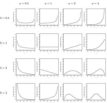
The beta distribution

The beta distribution is a distribution that has very flexible shapes with two parameters a and b, shown in Figure 3.2, from flat to narrow curves. Let X

be the random variable that follows a beta distribution with non-negative parametersa andb,X ∼Beta(a, b). Its probability density function is given by

f(x) = 1

B(a, b)x

(35)

a= 0.5 a= 1 a= 2 a= 4

b= 0.5

0.0 0.2 0.4 0.6 0.8 1.0

0 1 2 3 4 5 6 x

0.0 0.2 0.4 0.6 0.8 1.0

0 1 2 3 4 5 6 x

0.0 0.2 0.4 0.6 0.8 1.0

0 1 2 3 4 5 6 x

0.0 0.2 0.4 0.6 0.8 1.0

0 1 2 3 4 5 6 x

b= 1

0.0 0.2 0.4 0.6 0.8 1.0

0 1 2 3 4 5 6 x

0.0 0.2 0.4 0.6 0.8 1.0

0 1 2 3 4 5 6 x

0.0 0.2 0.4 0.6 0.8 1.0

0 1 2 3 4 5 6 x

0.0 0.2 0.4 0.6 0.8 1.0

0 1 2 3 4 5 6 x

b= 2

0.0 0.2 0.4 0.6 0.8 1.0

0 1 2 3 4 5 6 x

0.0 0.2 0.4 0.6 0.8 1.0

0 1 2 3 4 5 6 x

0.0 0.2 0.4 0.6 0.8 1.0

0 1 2 3 4 5 6 x

0.0 0.2 0.4 0.6 0.8 1.0

0 1 2 3 4 5 6 x

b= 4

0.0 0.2 0.4 0.6 0.8 1.0

0 1 2 3 4 5 6 x

0.0 0.2 0.4 0.6 0.8 1.0

0 1 2 3 4 5 6 x

0.0 0.2 0.4 0.6 0.8 1.0

0 1 2 3 4 5 6 x

0.0 0.2 0.4 0.6 0.8 1.0

0 1 2 3 4 5 6 x

[image:35.595.138.499.125.470.2]

Figure 3.2: Beta densities with various values ofaand b.

for 0< x <1 where the beta function is defined as

B(a, b) = Γ(a)Γ(b)

Γ(a+b).

The gamma function is defined as Γ(a) = R∞ 0 u

a−1_e−u_du_if_a_{is a non-integer.}

If a is an integer the gamma function is a simple factorial function, Γ(a) = (a−1)!.

(36)

distri-Statistical Background 3.1 Distribution functions

butions. A k-parameter exponential family density can be written as

f(x, θ) =r(x)η(θ) exp

k

X

i=1

θipi(x)

.

The beta distribution thus can be shown is a two-parameter exponential family with r(x) = 1, η(θ) = Γ(a+b)/(Γ(a)Γ(b)), θ = (a−1, b−1)0 and

p(x) = (log(x),log(1−x))0 where log(·) is the natural logarithm,

f(x, θ) = Γ(a+b)

Γ(a)Γ(b)exp n

(a−1) log(x) + (b−1) log(1−x)o

= 1

B(a, b)x

a−1₍₁₋_x₎b−1_,

The expected value of a beta random variable is E(X) =a/(a+b), and the variance is var(X) = ab/[(a+b)2₍_a₊_b_{+ 1)].}

3.1.3 Joint distribution

The Sarmanov distribution

One lesser known family of bivariate distribution is the family introduced by Sarmanov which appeared in Doklady (Soviet Mathematics) in 1966 (Lee, 1996). Define X1 and X2 as the random variables and f1(x1) and f2(x2) as the marginal probability density functions of X1 and X2, respectively. Let

µi be the mean of Xi and σi the standard deviation fori= 1,2. The general function of the joint density function is

h(x1, x2) = f1(x1)f2(x2)

1 +ωφ1(x1)φ2(x2)

(37)

where ω is a real number that satisfies the condition 1 +ωφ1(x1)φ2(x2)≥0 andφi(xi) is a nonconstant mixing function bounded by

R∞

−∞φi(xi)fi(xi)dxi =

0 (i= 1,2) for all values of x1 and x2.

The correlation coefficient of X1 and X2 is given by ρ =ωσ1σ2 where ω satisfies the condition

max

₋

1

µ1µ2

, −1

(1−µ1)(1−µ2)

≤ω ≤min

1

µ1(1−µ2),

1

µ2(1−µ1)

.

Therefore,X1 andX2are positively correlated ifω >0; negatively correlated

if ω < 0; and independent if ω= 0.

In her paper, Lee (1996) discussed the properties and applications of the Sarmanov’s family of bivariate distribution. Of relevance to this thesis is the case where the marginals of the bivariate distribution follow the beta distributions. Let Xi be a random variable that follows a beta distribution with parameters ai and bi, that is, Xi ∼Beta(ai, bi), for i = 1,2. Since the sample space of the random variable is contained in [0,1], Lee proposed the mixing function to be

φi(ui) = xi−µi,

where µi =ai/(ai+bi). Therefore, the bivariate density ofX1 and X2 is

h(x1, x2) = f1(x1)f2(x2)

1 +ωx1−

a1

a1+b1

x2−

a2

a2+b2

, (3.5)

(38)

range

max

−(a1+b1)(a2+b2)

a1a2

,−(a1 +b1)(a2+b2)

b1b2

≤ω

≤min

(a1+b1)(a2 +b2)

a1b2

,(a1+b1)(a2+b2)

a2b1

⇔ −(a1+b1)(a2+b2)

max{a1a2, b1b2}

≤ω≤ (a1+b1)(a2+b2)

max{a1b2, a2b1}

.

In the same paper, Lee extended the family of Sarmanov’s bivariate distri-bution to the multivariate case. Let Xi be a random variable with marginal density function fi for i= 1,2, . . . , k then the k-variate joint density is

h(x1, . . . , xk) =

_Yk

i=1

fi(xi)

1 +RΩk(x1, . . . , xk)

, (3.6)

where

RΩk(x1, x2, . . . , xk) =

k−1 X

i1=1

k X

i2=i1+1

ωi1,i2φ(xi1)φ(xi2)

+ k−2 X

i1=1

k−1 X

i2=i1+1

k X

i3=i2+1

ωi1,i2,i3φ(xi1)φ(xi2)φ(xi3)

+· · ·+ω1,2,...,k k Y

i=1

φ(xi),

and Ωk = {ωi1,i2, ωi1,i2,i3, . . . , ω1,2,...,k} is a set of real numbers satisfying the

condition 1 +RΩk(x1, x2, . . . , xk)≥0. If all of the values ofω’s (each element

(39)

Statistical Background 3.2 Bayes’ theorem

3.2 Bayes’ theorem

Suppose that a parameterθdoes not have some fixed value but is random. Its probable value is quantified in a probablity density function known as prior density, fΘ(θ). The random variable X depends on the unknown parameter

θ in a known way and having observed some data X =x the dependency is expressed by a density function, fX|Θ(x|θ), which is known as the likelihood function. The new opinion of the parameter θ is updated and by the Bayes’ theorem it is

fΘ|X(θ|x) =

h(x, θ)

fX(x)

= fX|Θ(x|θ)fΘ(θ)

fX(x)

, (3.7)

whereh(x, θ) is the joint density ofX andθ. The functionfΘ|X(θ|x) is called the posterior density. The marginal density of X is obtained by integrating

h(x, θ) over the sample space of θ,

fX(x) =

Z

h(x, θ)dθ =

Z

fX|Θ(x|θ)fΘ(θ)dθ. (3.8)

The marginal distribution of X is also called the predictive distribution.

3.2.1 Normal mean

The Bayes’ theorem is one of the fundamental tools in the Bayesian analysis. Following are two illustrations of using Bayes’ theorem to infer the unknown parameter of a random variable that follows a known distribution. Let X be a random variable that follows a normal distribution with unknown mean θ

(40)

also follow a normal distribution with known mean µ and variance τ2_{. The} prior density of θ is

fΘ(θ) = 1

τφ

θ−µ

τ

= √ 1

2πτ2 exp

−(θ−µ)

2 2τ2

,

and the likelihood function of X is

fX|Θ(x|θ) =

1

√

2πσ2exp

−(x−θ)

2 2σ2

.

The marginal density ofX is thus,

fX(x) =

Z ∞

−∞

fX|Θ(x|θ)fΘ(θ)dθ

= Z ∞

−∞

1 2πτ σexp

− 1

2τ2_σ2(τ

2₍_x₋_θ₎2₊_σ2₍_θ₋_µ₎2₎ dθ = Z ∞ −∞ 1 2πτ σexp

− 1

2τ2_σ2

θ− τ

2_x₊_σ2_µ

τ2₊_σ2

2

(τ2+σ2)

+ τ

2_σ2

τ2₊_σ2(x−µ)

2

dθ

= √ 1

2πτ2_σ2 exp

− 1

2(τ2 ₊_σ2₎(x−µ) 2 × Z ∞ −∞ 1 √

2πexp

− τ

2₊_σ2 2τ2_σ2

θ− τ

2_x₊_σ2_µ

τ2₊_σ2

2

dθ

= √ 1

2πτ2_σ2 exp

− 1

2(τ2 ₊_σ2₎(x−µ) 2

·

r

τ2_σ2

τ2₊_σ2

= _p 1

2π(τ2 ₊_σ2₎exp

− 1

2(τ2₊_σ2₎(x−µ) 2

. (3.9)

(41)

letλ= (τ2_x₊_σ2_µ₎_/₍_τ2₊_σ2_{) and}_ν _{= (}_τ2_σ2₎_/₍_τ2₊_σ2_{), the posterior density} of θ is

fΘ|X(θ|x) =

h(x, θ)

fX(x)

=

expn−(θ−λ)2₍_τ2₊_σ2_{) +}_ν₍_x₋_µ₎2_/₍₂_τ2_σ2₎o_/₍₂_{πτ σ}₎

expn−(x−µ)2_/₍₂₍_τ2₊_σ2₎₎o_/p

2π(τ2₊_σ2₎

= √1

2πν exp

n

− 1

2ν(θ−λ)

2o_. _(3.10)

The posterior distribution of the random parameter θ is also a normal dis-tribution but with mean λ and varianceν.

3.2.2 Binomial distribution

For the second illustration, let X be a discrete random variable and assume that it follows a binomial distribution such that X|p ∼ Bin(n, p). The parameter p is assumed to be random and as 0< p <1 a convenient choice for the prior distribution is a beta distribution. Assume that p∼Beta(a, b) with known parametersaandb. From equations (3.1) and (3.4) the marginal density of X is therefore,

fX(x|a, b) =

Z 1 0

fX|p(x|p)fp(p)dp

= n x 1

B(a, b)

Z 1 0

pa+x−1(1−p)b+n−x−1dp

=

n x

B(a+x, b+n−x)

(42)

The marginal distribution of X is known as the beta-binomial distribution with index n, and parameters a, and b.

The posterior density ofp given data xis

fp|X(p|x) =

fX|p(x|p)fp(p)

fX(x)

= 1

B(a+x, b+n−x)p

a+x−1₍₁₋_p₎b+n−x−1_, _(3.12)

which has the same form as a beta distribution. The posterior distribution of p given x is thus a beta distribution with parameters (a+x, b+n−x).

In both examples, it is shown that ifXis normal with parameterθ which prior distribution is also normal, its posterior distribution is likewise a normal distribution but with different parameters. Similarly, if X is binomial with parameter p and if it follows a beta distribution, its posterior distribution is also a beta distribution with different parameters. In general, if L(θ;x) is a likelihood function and fΘ is a prior distribution belongs to a family of G where the posterior density

fΘ|x(θ|x)∝fΘ(θ)L(θ;x),

(43)

3.2.3 Sarmanov distribution

The next example is based on the k-variate joint distribution from the Sar-manov’s family. LetXibe a random variable that follows a binomial distribu-tion with index ni and an unknown parameter pi (i = 1,2, . . . , k). Suppose that the likelihood functions of X1, X2, . . . , Xk are independent from each other, then the joint conditional density, denoted byhX|p(x1, . . . , xk|p1, . . . , pk), is the product of all the likelihood functions,

hX|p(x1, . . . , xk|p1, . . . , pk) =

k Y

i=1

fX|p(xi|pi) = fX|p(x1|p1). . . fX|p(xk|pk).

(3.13) Suppose that pi is a random variable and has a beta distribution with known parametersaiandbi, and let the joint distribution ofp1, p2, . . . , pk fol-lows the k-variate Sarmanov’s family as seen in (3.6). Denote hp(p1, . . . , pk) as the joint density ofpi’s and let the mixing function beφi(pi) =xi−µiwhere

µi = ai/(ai +bi) is the expected value of the beta distribution. Therefore, the unconditional joint density ofX1, X2. . . , Xk, denoted by hX(x1, . . . , xk), is

hX(x1, . . . , xk) =

Z · · ·

Z k Y

i=1

fX|p(xi|pi)h(p1, . . . , pk)dp1· · · dpk,

an iterated integral. The detailed working of the integration by parts is shown in Appendix A. From equation (A.8), the unconditional joint density

of X1, . . . , Xk is

hX(x1, . . . , xk) =

_Yk

i=1

fX(xi)

(44)

where fX(xi) = n_x_ii

Beta(ai +xi, bi +ni −xi)/Beta(ai, bi) is the marginal

density of Xi and

DΩk(x1, . . . , xk) =

k−1 X

i1=1

k X

i2=i1+1

ωi1,i2ψ(xi1)ψ(xi2)

+ k−2 X

i1=1

k−1 X

i2=i1+1

k X

i3=i2+1

ωi1,i2,i3ψ(xi1)ψ(xi2)ψ(xi3)

+· · ·+ω1,2,...,k k Y

i=1

ψ(xi),

where the function ψ is defined as ψ(xi) = (xi−µini)/(ai+bi+ni). From equations (3.6), (3.13), and (3.14) the joint posterior density is

hp|X(p1, . . . , pk|x1, . . . , xk)

= hX|p(x1, . . . , xk|p1, . . . , pk)hp(p1, . . . , pk)

hX(x1, . . . , xk)

=

k Y

i=1

fX|p(xi|pi)fp(pi)

fX(xi)

1 +R_Ω

k(p1, . . . , pk)

1 +DΩk(x1, . . . , xk)

= 1 +RΩk(p1, . . . , pk)

1 +DΩk(x1, . . . , xk)

k Y

i=1

fp|X(pi|xi) (3.15)

(45)

Statistical Background 3.3 Hypothesis testing and power function

3.3 Hypothesis testing and power function

The theory of statistical inference is broadly divided into two branches, namely, estimation and hypothesis testing. It is the latter branch that is discussed in this section. Due to the inherent variability in observing an outcome in each situation, a probability distribution is used to describe the variability. However, the true probability distribution is also unknown to us. The inference problem is thus to infer something of the true distribution or the true parameter. Observations from a certain sample space are more likely to belong to some known distributions, for example, continuous vari-ables may follow the normal distribution or the beta distribution and discrete random variable may tend to follow the binomial distribution. Therefore, for this thesis, it is assumed that the inherent variability of observations are adequately explained by a known probability distribution. The inference problem is then to make use of the observed outcomes to estimate the true parameter.

We generally wish to test a statement that the true parameterθbelongs to a subset of the parameter space Θ. This statement is known as a hypothesis. The testing of the hypothesis is to use statistical methods to check if the observations are consistent with the stated hypothesis or not. A statistical rule is used to assign “each possible observation to one of two exclusive categories: ‘consistent with the hypothesis under consideration’ and ‘not consistent with this hypothesis”’ (Silvey, 1975, pp. 95).

(46)

which states that the parameter θ belongs toω which is a subset of Θ. The other hypothesis is simply known as the alternative hypothesis which states that the parameter θ does not belong to the subset ω but belongs to Θ−ω. If there is only one element in ω, the hypothesis is known as a simple null hypothesis because it is in its simplest form, and similarly, if there is only one element in Θ−ωthe alternative hypothesis is a simple alternative hypothesis. Suppose that the elements in ω and Θ−ω are θ0 and θA, respectively, the hypotheses can be formulated as

H0 :θ =θ0 against H1 :θ =θA,

where the statement H0 is the null hypothesis and H1 is the alternative hypothesis. The null hypothesis is always assumed to be true until proven to be otherwise. The statistical rule to reject H0 is called a statistical test.

Two possible decisions can be made based on the observed data at the end of the trial: (1) reject the null hypothesis, or (2) do not reject the null hypothesis. Inevitably, errors may occur when rejecting or not rejecting H0. The type I error is an error incurred when the null hypothesis is rejected when it is true. Another type of error that can be incurred is the type II error. It is an error incurred when the null hypothesis is accepted when it is false. The probability of incurring the type I error is usually capped at a predetermined value α such that,

(47)

and similary, the probability of incurring the type II error is capped by a predetermined value β,

Pr(Non-rejection ofH0|H1 is true)≤β.

The probability that the null hypothesis is rejected when it is false is called the power of the test and it is simply 1−β. Although the choice ofαcould be arbitrary, it is customary to have αat small values such as 0.1, 0.05, or 0.01. Similarly, the customary values of β are 0.2, 0.1, or 0.05. Correspondingly, the power of the test is 0.8, 0.9, or 0.95, respectively.

If X1, X2, . . . , Xn are n independent continuous random variables and

each is normally distributed with unknown mean θ and known variance σ2_, letX=Pn

i=1Xi/n, thenX ∼N(θ, σ

2_/n_{). Let (}_x

1, x2, . . . , xn) be the sample

ofX1, X2, . . . , Xn. It is desired to test whether the true mean is equal to some

constants θ0 or θA. The simple hypotheses are

H0 :θ =θ0 against H1 :θ =θA.

The decision to either rejectH0or not is made on the basis of the test statistic upon observing the responses at the end of the trial. The test statistic is most powerful if X > c where c is some constant such that the size of the test is

α,

Pr(X > c) =α.

(48)

distribution, Z ∼N(0,1). Solving for cunder the null hypothesis,

Pr(Reject H0|θ =θ0) =α

⇔ Pr(X > c|θ =θ0) =α

⇔ Pr

X−θ

p

σ2_/n >

c−θ

p

σ2_/n

θ=θ0

=α

⇔ Pr

X−θ0

p

σ2_/n >

c−θ0

p

σ2_/n

=α

⇔ Pr

Z > _pc−θ0

σ2_/n

=α

⇔ 1−Φ

c−θ0

p

σ2_/n

=α

⇔ c=z1−α

p

σ2_/n₊_θ

0 (3.16)

where zγ is the lower 100γ percentile of the standard normal distribution. The computation of the power on the other hand is important when designing a trial. The power calculation is one of the standard statistical methods in determining sample size. Under the alternative hypothesis, X ∼

N(θA, σ2/n) and from equation (3.16),

Power = Pr(Reject H0|θ =θA)

1−β = Pr

X−θ

p

σ2_/n >

c−θ

p

σ2_/n

θ =θA

= Pr

Z > z1−α

p

σ2_/n₊_θ

0 −θA p

σ2_/n

= 1−Φ

z1−α−

θ_A−θ₀ p

σ2_/n

(49)

Statistical Background 3.4 Assurance

of n and if n is fixed, it can be evaluated as a function of θA.

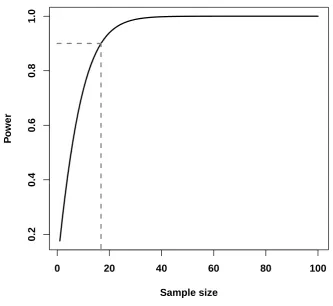
As an example, a new bronchodilator for asthma control is ready to be put on clinical trials. The primary endpoint is the mean percentage change in FEV1 from baseline. Let θ be the difference of mean change between the new bronchodilator and a placebo. The new bronchodilator is considered to be effective in controlling asthma if the mean change difference is at least 10 percent, that is, let θ0 = 0 (there is no difference in mean change between the new bronchodilator and placebo) and θA = 10. Assume that the popu-lation standard deviation is known and fixed at σ = 14, and the size of the hypothesis test is α = 0.05. The power function which for a fixed θA is a function of n is shown in Figure 3.3. According to the figure, in order to achieve a power of at least 90%, the sample size has to be at least 17.

3.4 Assurance

(50)

0 20 40 60 80 100

0.2

0.4

0.6

0.8

1.0

Sample size

P

o

[image:50.595.156.490.171.477.2]

wer

Figure 3.3: Power as a function of n.

for θ. Therefore, the power is now a kind of average power and is called as-surance. Denote the assurance as A and from equation (3.17) the assurance is given by

A=E(Power) = Z

Θ

1−Φ

z1−α−

θ−θ₀ p

σ2_/n

fΘ(θ)dθ, (3.18)

(51)

3.4.1 Normal distribution

As an illustration, consider a random variable X whose likelihood is X|θ ∼

N(θ, σ2/n) where the variance σ2/n is known and θ is a random parameter such that θ ∼ N(µ, τ2) where µ and τ are known. Similar to the workings in equation (3.9), the marginal distribution of X can be shown to be normal with mean µ and variance (τ2₊_σ2_/n_{). Thus, the assurance is}

A= Pr(X > z1−α p

σ2_/n₊_θ

0)

= PrZ > z1−α

p

σ2_/n₊_θ

0−µ

τ2₊_σ2_/n

= 1−Φz1−α− p

n/σ2₍_µ₋_θ

0) p

1 +nτ2_/σ2

, (3.19)

which is a function of n.

3.4.2 Binomial distribution

For another illustration, letX1andX2 be binary random variables andX1 ∼

Bin(n1, p1) andX2 ∼Bin(n2, p2). Under the frequentist setting, it is desired to test the hypothesis,

H0 :p1 =p2 against H1 :p1 6=p2.

A simple measurement to test the hypothesis isδ =p2−p1 which lies between

−1 and 1. However, the restricted parameter space ofδmay lead to anomalies

(52)

defined as

θ= logp2(1−p1)

p1(1−p2)

,

and because the log odds ratio lies between−∞and∞, it is a more appealing measurement than the simple measurement of difference of proportions. The hypotheses are now rewritten as

H0 :θ = 0 against H1 :θ6= 0,

The score statistic for θ is

B = n1S2−n2S1

n , (3.20)

and the Fisher’s information is

V = n1n2S(n−S)

n3 , (3.21)

where Si is the number of successes out of ni for i = 1,2, S =S1 +S2 and

n = n1 +n2. The score statistic B is approximately normally distributed with mean θV and variance V, B ∼ N(θV, V). Assume that n1 = n2, and that the probability of success of the whole trial is ¯p= (p1+p2)/2. For large sample size, S ≈np¯, and so the equation (3.21) becomes

V ≈ np¯(1−p¯)

(53)

For a two-sided hypothesis, under the null hypothesis,

Pr(B > c|θ = 0) =α/2

⇔ PrZ > c−√θV

V

=α/2

⇔ 1−Φ√c

V

=α/2

⇔ c=z1−α/2

√

V .

Let θA be the anticipated log odds ratio to be detected from the trial and it is one of the parameters in the alternative space Ω−ω. The power of the trial is,

1−β = Pr(B > c|θ=θA)

= Pr

Z > z1−α/2

√

V −θAV

√

V

= PrZ > z1−α/2−θA

√

V

= 1−Φz1−α/2−θA √

V.

Assume that p1 is a fixed constant while p2 is a random parameter that follows a beta distribution with fixed parameters a and b. The power now has to be averaged over all possible values of p2,

A=

Z 1 0

1−Φz1−α/2−θ

√

V

f2(p2)dp2

= Z 1

0

1−Φz1−α/2−log

p₂(1−p₁)

p1(1−p2)

r

np¯(1−p¯)

4

f2(p2)dp2,

(54)

Statistical Background 3.5 Decision theory

which is also a function of n and can only be evaluated numerically.

3.5 Decision theory

The simple hypothesis testing is one of inference problems where the results from the trial is used to infer the value of the unknown true parameter θ of a random variable X. In a broad sense, it is also a decision problem. After the collection of observations, a decision is made from a choice of two. These decisions are:

d0: The hypothesis that the unknown θ belongs to ω is true.

d1: The hypothesis is false.

Another technique of formally making informed decision is the statistical decision theory. Decision theory is concerned about making decision un-der uncertainty and each decision has its consequence and “value”. Unun-der the uncertain circumstances, a decision has to be made such that it is the best possible one with the knowledge that the worst scenario could happen (Pratt et al., 1995, Ch. 1).

(55)

Action T

Action A

Success

Failure

G(T,q1)

G(T,q2)

[image:55.595.178.485.116.362.2]

G(A)

Figure 3.4: A simple decision tree for a phase II trial.

For the review of the decision theory, a simple illustration is used. Sup-pose that a new treatment is available for a phase II clinical trial then there are two possible actions to choose:

Action T: Try the new treatment in the phase II trial, or

Action A: Do not try the new treatment in the phase II trial.

There are two possible states of nature from the new treatment:

θ1: The new treatment is effective,

θ2: The new treatment is not effective.

(56)

that is, a failure, it has 0 unit of gain. Let the cost of starting a trial be m

which is relative to the one unit of gain. The gain of taking action T and if the treatment is effective is, G(T, θ1) = 1−m, and if the treatment is not effective it is, G(T, θ2) = −m. If action A is taken, then there is no cost incurred and so G(A, θi) = 0 for i= 1,2 (Hilden, 1990). The utility table is as shown in Table 3.1.

Suppose that the probability of the trial being a success is p and the probability of it failing is 1 − p. The expected utility function of action

a ∈ {T, A} is

G(a) = X θ∈Θ

G(a, θ)p(θ).

Thus, the expected utility for action T is

G(T) = p(1−m)−(1−p)m =p−m,

and the expected utility for action A is

G(A) = 0.

Therefore, if the probability of success is greater than the relative start-up cost, the optimal action is action T, otherwise, action A. For example, if the relative start-up cost is 0.02, then if p > 0.02, the treatment should be put on trial but if p <0.02 then the trial should be abandoned.

(57)

Table 3.1: Utility table for a phase II trial.

State of nature

Action θ1 θ2

T 1−m −m

A 0 0

responses from these patients are available in a sequential order, the analysis to test the hypothesis is still performed at the end of the trial—after the data from the last patient has been obtained. Nevertheless, due to the sequential nature there is a feasibility to analyse the data as they are made available especially if it deems more advantageous to do so. One of the advantages of doing sequential analysis is the flexibility to stop a trial early.

After each sequential analysis, there is a possible set of decisions to be made: 1) to stop the trial because the new treatment is not efficacious and thus subject fewer patients to the inferior treatment, 2) to stop the trial and recommend the drug for larger confirmatory trials or for marketing, thus making it available for more patients quicker, or 3) to recruit more patients as the results are inconclusive to decide if the treatment is effective or not.

(58)

the chance of claiming efficacy when in fact it is not. Another method is to construct stopping boundaries where a set of critical values are determined before the trial begins. The observed data are used to calculate the test statistics and then compared with the critical values to determine if the trial should stop or continue.

3.5.1 Backward induction

The formulation of the design of sequential clinical trials to be discussed in Chapters 6 and 7 is based on the Bayesian decision theoretic approach and thus, will be discussed in slightly greater length here. For an illustration, in a clinical trial, n1 patients are recruited in the first stage and upon the collection of observations a decision is made from a choice of:

Action R: Recruit another patient, or

Action A: Abandon the trial.

If action R is taken, n2 patients are recruited in the second stage and a decision to take action R or A is made from the accumulated responses. At stage k the decision making is based on the accumulated data from

n1, n2, . . . , nk patients and either the trial terminates or continue by

recruit-ing nk+1 patients. Suppose that there are only N patients eligible for trial and N = Pk

i=1ni. If all N patients were observed, then the only action available is to terminate the trial, action A. The sequential decision tree is shown in Figure 3.5.

(59)

Action R Action A

Action A

1st_stage ₂nd_{stage …} ₍_k– 1)-th stage _k_{-th stage}

Action R

Action A Action R

[image:59.595.163.505.134.386.2]

Action A

Figure 3.5: A simple sequential decision tree for a phase II trial.

the first stage of the observation (DeGroot, 1970, Ch. 12). Analogous to the simple decision tree, the gain function of recruiting n1 patients must be greater than the gain function of not recruiting in order for the trial to commence. Based upon the observation fromn1patients, if there is benefit in recruitingn2 patients for more information than not recruiting, then action R should be taken. Otherwise, action A. In the former scenarion2 patients are recruited in the second stage and based on the accumulated information from

(60)

patients should be recruited to the k-th stage before the trial terminates. Let xi be the observed events from the i-th stage, i = 1,2, . . . , k. The gain function at the k-th stage can be denoted by G(A|x1, . . . , xk) because only action A is available after obtaining information from all N patients. At the (k−1)-th stage, the gain function of action R is

G(R|x1, . . . , xk−1) =

X

xk

G(A|x1, . . . , xk)f(xk|x1, . . . , xk−1),

which depends on the benefit of recruiting nk more patients and the possi-ble values that may be observed. The expression f(xk|x1, . . . , xk−1) is the function of the possible observed events in the k-th stage given the observed events x1, x2, . . . , xk−1.

Similarly, the gain function of action A depends on all thex1, x2, . . . , xk−1 observations, denoted by G(A|x1, . . . , xk−1). If

G(R|x1, . . . , xk−1)> G(A|x1, . . . , xk−1),

then the optimal decision is to take action R and if otherwise, action A. By working recursively back to the first stage, an optimal decision can be made for all possible observations from n1 patients.

As described by Lindley (1961), the optimality problem at each present stage is solved by considering the optimum future. The sequential recruit-ment of patients by blocks ofni’s is known as group sequential. Whenni = 1,

for i = 1,2, . . . , k the sequential recruitment is called fully sequential. In

(61)

Statistical Background 3.6 Concluding remarks

for a series of trials are based on fully sequential.

3.6 Concluding remarks

In the design of clinical trials, one of the key components is to have an appropriate sample size such that the minimally clinical accepted efficacy is detected with small errors. Some of the methodology to determine sample size is discussed in the following chapter. Most of the designs regard each clinical trial individually even though the success or the failure of one may have an impact on subsequent trials. A new design for a series of trials is proposed in Chapter 5 so that the optimality of the whole of the project development is considered. Following on that, a series of sequential trials with sequential sampling is proposed in Chapter 6. Patients are recruited sequentially and observations from the patients are then used to support if the current trial should continue recruitment, stop and initiate another clinical trial or abandon the development programme. Treatments targeting the same population may be more similar and thus may be correlated. The design for a series of sequential trials is therefore extended by considering the correlation between treatments (Chapter 7).

(62)

Statistical Background 3.6 Concluding remarks

(63)

Chapter 4 Sample Size Determination

Due to the inherent biologic variations in patients presented with the same condition it is necessary to have a group of patients in clinical trials. The results from the sampled patients are consequently used to infer how the treatments may behave in the population. Thus, one of the fundamental issues in the design of a clinical trial is the number of patients that should be sampled. On the one hand, a sample size that is too large may delay the treatment from being made available to the population when it has shown some minimum clinical efficacy. On the other hand, an inadequate sample size may not be able to draw a valid conclusion thus, subjecting patients unnecessarily to “questionable” treatments.

(64)

Sample Size Determination

the experimental treatment is compared against a known value of an his-torical control. The designs discussed in the later sections thus include both controlled (two-arm) and uncontrolled (one-arm) trials, and the primary end-point is assumed to be either a continuous variable or a binary variable.

This thesis assumes that the trial’s primary outcome, X, is a random variable that has a known form of a probability distribution function with an unknown parameter θ. The probability density function (or equivalently the probability mass function for a discrete variable) is represented by f(x|θ). Patients’ outcomes are independent of each other and so each random vari-able is assumed to be independently and identically distributed with the same probability density function, f(x|θ).

The sample size is determined based on the analysis of the primary end-point that is to be done at the end of the trial (ICH, 1998), that is, an inference on parameter θ is made. Issues such as patient withdrawal and protocol violation may affect the actual number of patients in a trial and thus, methods that deal with these issues are employed alongside the com-mon sample size calculation formulations to determine the minimum sample size that is necessary. However, these methods will not be discussed in this thesis.

Designing a series of clinical trials

Library Declaration and Deposit Agreement

Designing a Series of Clinical

Trials

by

Siew Wan Hee

A thesis submitted in partial fulfilment of the requirements for

the degree of

Doctor of Philosophy in Health Sciences

Contents

I

Background

5

II

Designs for a Series of Hybrid Trials

85

III

Designs for a Series of Decision-Theoretic

Tri-als

106

IV

Summary

172

V

Appendices

183

List of Tables

List of Figures

Acknowledgements

Declaration

Abstract

Thesis Overview

Part I

Chapter 1

Clinical Trials

Chapter 2

Asthma

2.1

Therapies for asthma

2.2

Outcome variables

Chapter 3

Statistical Background

3.1

Distribution functions

3.1.1

Discrete random variables

3.1.2

Continuous random variables

3.1.3

Joint distribution

3.2

Bayes’ theorem

3.2.1

Normal mean

3.2.2

Binomial distribution

3.2.3

Sarmanov distribution

3.3

Hypothesis testing and power function

3.4

Assurance

3.4.1

Normal distribution

3.4.2

Binomial distribution

3.5

Decision theory

3.5.1

Backward induction

3.6

Concluding remarks

Chapter 4

Sample Size Determination