Design of an Integrated Long
Distance Transportation, Ordering
and Inventory Quantity
Optimization Tool
Bachelor Thesis
Industrial Engineering & Management
Management summary 4
Purpose of research 4
Problem Statement 4
Proposed solution and preliminary results 4
Conclusion 4
Recommendations 4
1. Introduction 5
1.1. Company 5
1.2. Management problem 5
1.3. Problem Identification 5
1.4. Core Problem 6
1.5. Research focus 7
1.6. Norm, reality and variables 7
1.7. Methodology - Problem solving approach 7
1.7. Criteria for the Solution 8
2. Current Situation 10
2.1. Responsible employees 10
2.2. Current ordering process 10
2.3. Effects on performance 11
3. Theoretical framework 11
3.1. Exploratory Systematic Literature Review 11
3.2. The Supply Chain from academic theory 12
3.3. The Economic Order Quantity (EOQ) 12
3.4. Dynamic Lot-Size Model 13
3.5. Demand 13
3.6. Optimization Models and Techniques 14
Deterministic Models 14
Stochastic Models 14
Economic Models 14
Simulation Models 14
3.7. Demand Forecasting Techniques 14
3.7.1. Extrapolation methods 14
Moving average 14
Exponential smoothing 14
3.7.2. Causal forecasting methods 15
Regression analysis 15
3.8. Forecast Error and Expected Accuracy 16
Mean Absolute Deviation 16
Mean Squared Error 16
Normal Distribution 16
4. Solution proposition 17
4.1. Selection of Technique 17
4.1.1. Deterministic vs stochastic model 17
4.1.3. Selection Forecasting Model 18
4.2. Assumptions and Limitations of the Models 19
4.2.1. Assumptions for the Supply Chain 19
4.2.2. Demand 19
4.2.3. Assumptions for the ordering quantity dynamic program 19 4.2.4. Assumptions for the Transportation Quantity Dynamic Program 19
4.2.5. Factors of the Forecasting Model 20
4.3. Dynamic Programming Model 20
4.4. Triple Exponential Smoothing Model 21
4.4.1. Standard TES formulas 21
4.4.2. Example calculations, forecast error and forecast accuracy 21
4.5. Overview of Input and Output Streams 22
4.6. Implementation in the Company 22
5. VBA Program 22
5.1. VBA Programming Approach 22
5.2. Program dashboard functions and usability 23
5.2.1. Forecast Dashboard 23
5.2.2. Transportation Schedule 24
5.2.3. Ordering Schedule 25
5.5. Validation Ordering and Transportation Model 25
5.6. Validation Forecasting Model 26
5.7. Implementation 26
6. Evaluation 27
6.1. Usability 27
6.2. Realization of the norm 27
7. Conclusion and recommendations 29
7.1. Conclusion of this research 29
7.2. Further research and optimization possibilities 29
7.2.1 Further validation with periodical data 29
7.2.2. Stochastic modeling approach 29
7.2.3. Linear Programming model 29
7.2.4. Extension of product ranges in the tool 29
7.2.5. Forecasting 30
8. Bibliography 31
9. Appendix 31
Appendix A - Systematic Literature Review 31
Appendix B - Conceptual Model and Overview of Design Process 39
Appendix C - Standard TES formulas 39
Appendix C - Specific example calculations 41
Émile Heijs
Student number: s1711865
Email address: [email protected] Telephone: 0640422836
Supervisory Committee
Lead Supervisor University of Twente Martijn Koot Msc
Email address: [email protected] Telephone: +31534896083
Second Reader University of Twente Nils Knofius Msc
Management summary
Purpose of research
The research described in this report proposes a method to optimize logistic processes within a small Dutch (4 FTE) wholesale company delivering high quality olive oil and derivatives to B2B clients. This research is done because, according to the management of the company, these processes were not performing according to their expectations. This research focuses on the transportation, ordering and inventory decisions within the company related to their most important product, referred to in this research as product X. This is a small and durable plastic single-serving container filled with a variety of different contents (such as extra virgin Italian olive oil) and is available in different sizes. The sale of product X contributes to about 70% of their revenue and is therefore the cornerstone of the company. This research aims to provide the company with an easily implementable solution to improve the logistics performance by substantiated decisions in this area.
Problem Statement
Product X is ordered and transported ad hoc from Italy in small quantities (1 to 4 pallets) and delivered straight to their clients in the Netherlands/Northern Europe. Every order is bought separately for a specific client, so no significant inventory is kept and no quantitative forecasting is done. In 2018 this meant 5% of the company’s revenue was spent on transportation of product X. Shipping one pallet is relatively expensive, but when combining pallets in a single transportation order these costs decrease exponentially. This is also true for the ordering cost of product X, and has therefore been included in this research. Additionally, these repetitive logistic actions demand a significant amount of time from employees. Mathematically substantiated decisions in the areas of ordering, transportation and inventory quantities combined into an integrated planning system are believed to reduce transportation and ordering cost while also decreasing order handling time. The core problem is defined as follows: In the current situation, quantity discounts on ordering and transportation quantities by using inventory are not utilized causing transportation costs to be 5% of revenue instead of the market average of 3%.
Proposed solution and preliminary results
The solution is proposed in the form of a simple to use Excel tool which provides the management with a demand forecast and an ordering and transportation planning. As a basis for the Excel planning tool a combination of three mathematical models have been used. Transportation and ordering quantities are found using an extension of the EOQ (dynamic lot-size model) solved over a multiple period planning horizon using the dynamic programming technique (DP). The deterministic demand for the dynamic programming models is calculated using a triple exponential smoothing forecasting model. The tool gives the company insight into transportation, order and inventory quantities that will minimize total cost over the planning horizon based on the demand pattern provided. When comparing the total cost of the schedule output of the tool to the current ad hoc strategy, using realistic input and an average ad hoc order size of 3 pallets, preliminary results show transportation costs can be reduced by more than 50%. This reduction achieves a decrease in transportation costs from 5% to 1.3% of the total revenue. Smarter investment in price discounted product (order more less often) is also estimated to achieve an efficiency gain of around 50% in investment cost for the scenarios tested.
Conclusion
In conclusion, a deterministic DP approach to solving a multi-periodic dynamic lot-size model for a certain planning period is likely to provide the company with significant savings in transportation costs and investment in product X. Still, the tool remains fast, user-friendly and easily implementable in existing logistic processes. This approach is therefore a useful stepping stone in improving their logistics performance rapidly..
Recommendations
The company is strongly advised to keep track of 2 weekly demand levels and order sizes for further validation purposes which could not be done in this research, since no periodical historical data was available; only total cost and revenue figures, transportation costs and the amount of units product X on one pallet were provided. Hence, expected cost reductions are calculated based on a number of assumptions (e.g. demand patterns, historical order sizes and investment costs). The lack of necessary data is an important side note to this research. After the right data has been tracked, the performance of the tool should be compared to historical situations where the demand and the decisions are known. Both with and without an optimization. In time, other products varieties and/or other transportation distances could be included in the Excel tool. Longer-term recommendations concerning this research are:
1. Introduction
In the first chapter of this thesis, the company and the management problem are introduced. Furthermore, after an analysis of the management problem, a core problem for this thesis is selected. Based on this core problem the problem solving approach is presented.
1.1. Company
The company for which this research has been conducted is a small Dutch wholesale company delivering high quality olive oil and derivatives (balsamic vinegar, sauces) to supermarkets, retail chains and restaurants. Their most important product range consists of small and durable one-dose plastic containers (available in three sizes: 8ml, 15ml and 24ml) filled with a variety of different contents, referred to in this research as product X. This innovative packaging concept was introduced by the company in 2012 and is very successful. The sale of product X contributes about 70% of their revenue and is therefore the cornerstone of the company. A few years ago they also started selling high quality olive oil delivered at home to regular customers via their webshop. They use special bottles for these very premium products. These products are available in a variety of different ‘flavours’ as well. This company sources product X from Italy. There is a liaison with one very big Italian production company (this producer is also shareholder), which produces product X sourcing olive oil from Italian farmers.
1.2. Management problem
At the moment of starting this research, the management came forward with the following problem: “The logistic processes within our company are not performing according to our expectations. The costs (transportation costs in particular) are too high and actions take too much time. With the rapid growth of the company in mind,
optimization of these processes is needed to make the company ready for the future.” (Mulder - 2018)
1.3. Problem Identification
Since the management problem above is very broad, an analysis of the logistical situation was performed to find a suitable core problem for this research. With respect to the logistic processes within the company outlined in the management problem, all underlying problems that the company experiences have been identified by working at the company for a few months, conducting interviews and analyzing their processes. Subsequently, these problems have been analyzed for cause and effect and placed in a problem cluster. In such a cluster, links between various problems can be found more easily. The Managerial Problem Solving Approach (MPSM) (Heerkens & van Winden - 2012) details three varieties of problems in the process of business problem solving: problems that are and problems that aren’t caused by other problems in the company and problems that cannot be influenced. Core problems are those problems which have no cause and can be influenced. At the company the selected problems affect three main parts of the business: the sale of product X, the sale of bottles and the company in general. In the figure 1 below, all identified problems are presented with their cause and effect relations and grouped by colour to easily see their distinction.
Figure 1: Problem cluster
1.4. Core Problem
To select an appropriate core problem, the core problems from the problem cluster will be examined further below. One by one all identified core problems are presented in more depth, to eventually select the problem which has the highest value for the company when solved..
As seen in the diagram, multiple problems referring to the olive oil glass bottle production and sale via the
webshop have become clear. The CEO plays an important role in the sales department of the company, but is the only one with the authority to make payments. Since the CEO is away a lot on business, delays in payments often occur. This has serious effects on the production of their glass bottles for example. Because the filling company will only start production when there are no unpaid bills. Delays in production of the olive oil for these bottles happens regularly as well. Often farmers in the south of Italy have trouble to deliver in time. The delivery of olive oil to the Netherlands can take up to six weeks. This is partly because of cultural differences and partly because of inadequate stocks. Lastly, the collection of all necessary order details to finish a client order can take a week or more. This is partly due to the amount of tasks the responsible employee has, and partly because of vague communication within the company and difficult insight in stock.
The most significant identified core problem in the logistic processes is found in the production and transportation process of product X. Since the revenue of the company heavily relies on the sale of this product, significant financial gains may be realized with improvements in this area. Despite the fact that until now no demand forecasting was done, management believes that the sales outlook for product X is very positive and demand will continue to grow. This means this product will likely remain important in the future. As becomes clear from the problem diagram, product X is ordered and transported ad hoc from Italy in small quantities (1 to 4 pallets) and delivered straight to their clients in the Netherlands/Northern Europe. Every order is bought separately for a specific client, so no significant inventory is kept. In 2018 this meant 5% of the company’s revenue was spent on transportation of product X, which is significantly higher than the market average of 3% (according to the accountant of the company). Shipping one pallet is relatively expensive, but when combining more pallets in one order these costs decrease exponentially. This is also true for the ordering cost of product X, and has therefore been included in this research. While this fact is known at the company, no research has yet been conducted to address it. Additionally, the ad-hoc ordering strategy and repetitive logistic actions demand a significant and unnecessary amount of time from employees. Mathematically substantiated decisions in the areas of ordering, transportation and inventory quantities combined into an integrated planning system are believed to reduce transportation and ordering cost while also decreasing order handling time. The core problem is defined as follows:
In the current situation, quantity discounts on ordering and transportation quantities using inventory are not utilized causing transportation costs to be 5% of the revenue instead of the market average of 3%.
1.5. Research focus
Having defined the core problem the research focus for this research can be defined. Within this focus, the suitability for academic research, correspondence with the IEM program and prospected practical utility and implementability of the solution for the company have been taken into account. This research confines itself to the transportation, ordering and inventory quantity decisions within the company for product X. The aim is to provide the company with an easily implementable solution to improve efficiency and logistics performance, and thereby reduce cost and realize financial savings.
1.6. Norm, reality and variables
The core problem can be defined in variables to evaluate the effect of the solution in this research. The variable which is chosen is: transportation cost. This variable is measured as a percentage of total company revenue. The norm and reality of this variable is defined as follows: the transportation cost of product X as a percentage of the total revenue was 5% in 2018. This percentage needs to decrease to at least 3% (Drost, market average according to accountant, CEO - 2018).
1.7. Methodology - Problem solving approach
This research is divided into six phases to provide structure and clarity based on the Managerial Problem Solving Approach (MPSM - Heerkens & van Winden - 2012). The MPSM is a systematic approach for solving
management problems and provides a predefined path to follow and eventually construct the right solution for the right problem.
Phase 1 - Problem Identification and description of the current situation (Ch. 1 & 2)
The core problem is already identified. Also, in this phase the current situation has been outlined, explaining the current process of ordering and transporting pallets. This is done in chapter 2. In this phase the knowledge questions below will be answered:
●
What does the current supply chain for product X look like?●
What is the effect of current ordering and transportation strategy of product X on the supply chainperformance?
Phase 2 - Exploration of theory and optimization solutions (Ch. 3)
Next, possibilities for optimization of the current situation have been explored. Criteria that the solution must meet were defined, and a review of theory in the area of the core problem was performed. In this phase the following knowledge questions are answered:
● What research is available on mathematical optimization of transportation, ordering (production)
and inventory quantities?
● What criteria does the solution have to meet?
● With respect to previous research and the IEM program, which are possible ways to provide a
solution to the core problem?
● How can a deterministic model be used in an uncertain future planning scenario?
● Which way of demand forecasting should be used?
● How can the accuracy of the forecast be measured?
Phase 3 - Selection of optimization approach and creation of mathematical model (Ch. 4)
Based on the criteria from the previous phase an optimization approach has been selected and with this approach a mathematical model is created. Also the following knowledge questions are answered:
● Which mathematical models are best to optimize the ordering and transportation processes at the
company?
● How can a mathematical optimization model be integrated best in the company for easy and
simple usability?
Phase 4 - Creation of mathematical model solver program (Ch. 5)
After answering the previous research question, a solver program has been constructed based on the mathematical model and criteria of the previous two phases.
Phase 5 - Experimentation and validation of model Ch. 5)
In this phase, the Excel tool is used to validate the model and experiment. In this phase the last two knowledge questions are answered:
● Can the validity of the model be proven?
● What conclusions can be drawn from the model using data from the company?
Phase 6 - Evaluation and recommendations (Ch. 6 & 7)
In the last phase the solution will be evaluated based on the results of the previous phase. Also, recommendations will be made for further research and improvement in the research area.
Regarding the phases and knowledge questions above, the main research question is as follows:
How can the decision process regarding order, transportation and inventory quantities for product X be substantiated to increase efficiency and reduce cost?
1.7. Criteria for the Solution
There are a number of criteria for the solution that have been taken into account:
1. There are no theoretically substantiated logistic process optimizations in place at the company around product X. This will bethe first time there is research done specifically to optimize logistics around product X. The solution, therefore, has to be suitable to act as a first step for the company in this department. The solution has to be easy to use and user friendly, have a high degree of credibility (corresponding well with the real situation, models must not be so difficult they cannot be understood at the company)
2. The solution has to provide an insight in more cost efficient transportation, order and inventory quantities to subsequently make decisions according to results. The KPI that is used is total transportation cost. (as a percentage of revenue)
give a complete and usable solution to the problem without needing additional work, time or investment shortly after implementation of this research..
4. The ease of implementation is paramount. The final solution must be simple to understand and easy to use by the company, as staff is only 4 fte. If the proposed solution is too complex or time consuming, it will not be used and the intended results will not be achieved.
5. The techniques used in the solution have to be directly linked to the Industrial Engineering and
Management program at the University of Twente and fit within the time available for this research, which is about 10 weeks.
2. Current Situation
This chapter will give a brief overview of the current situation regarding the logistics around product X at the company. It will outline the responsible employees, the supply chain and the specific processes within the company.
2.1. Responsible employees
The company consists of the CEO, three full-time employees and one part-time employee. Within the company, the processes around product X are performed by the CEO and the account manager. This, however, is not their only responsibility. They both have a great variety of tasks, the most important of which is in the sales department (getting new clients). This means traveling often, keeping in contact with their B2B partners and biggest clients and selling product X or other products to new organizations.
2.2. Current ordering process
At the moment Product X is ordered ad hoc from Italy in mostly small quantities (1 to 4 pallets) and transported straight to the customer in the Netherlands/northern Europe. In 2018 this meant 5% of their revenue was spent on transportation of product X. Shipping one pallet is relatively expensive but when combining pallets in one order these costs decrease exponentially. Transportation is therefore significantly cheaper when more pallets are transported at once. This is also true for the purchasing price of product X. When product X is ordered in greater quantities at once, quantity discounts can be utilized and less investment in product is needed per unit of product X. The current process around the ordering and transport of product X is demand driven and therefore the
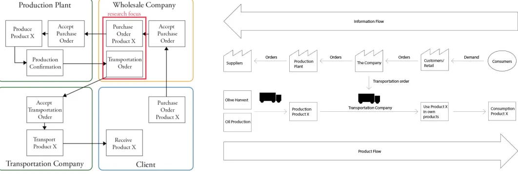
company does not keep inventory as every order is ordered separately. Currently, the only stock the company has is mandatory inventory for a client in the UK and one or two pallets at their office. Inventory is not used as a buffer for example while there are multiple interesting options for the company to start keeping inventory, either in the Netherlands or in Italy. Since product X can be ordered immediately when an order arrives via email, no demand forecasting is conducted. Since the company is relatively new and small, no real optimizations within this process have been conducted. A step by step description of the process as well as a detailed diagram are presented below:
1. The company receives an email with an order for a specific amount and variety of product X 2. A production order of this product is made and is sent to the production plant via email 3. Every order is printed as well and stored in a dossier.
Figure 2 & 3: Total supply chain overview and Value Stream Map
2.3. Effects on performance
The process above has certain effects on the supply chain performance of product X:
1. Handling each order separately → demands unnecessary time from employees while being repetitive and easy work.
2. Ad hoc investment in product X → very difficult to make use of quantity discounts at production plant 3. Rarely combining transportation of pallets → also not benefiting from quantity discounts in transportation 4. No use of inventory → low inventory risk → no buffer facing problems with late production etc., so
expensive alternative solutions are used (such as priority transport or last minute production in the Netherlands)
5. No tracking of periodical demand → no insight into more (cost/time) efficient ways of working 6. No demand forecasting → no insight into more (cost/time) efficient ways of working
The effects described above, especially the separate handling of orders and having no inventory (inventory could be a possibility in both Italy and the Netherlands), correspond well with the problem cluster from the previous chapter. This research aims to provide the company with a more efficient process to make decisions that combine multiple different orders in a smart way and save costs. A planning tool integrating transportation, ordering and inventory quantities is likely to reduce order handling time, utilize quantity discounts and use inventory as a buffer.
3. Theoretical framework
In this chapter, the existing research on the combination of transportation, ordering and inventory quantity will be explored using a systematic literature review. The results from the review will be used to define a number of concepts and theories in this research area, that can be used to develop a solution to the core problem. The abstracts that are selected for the development of the final solution will be explained in the beginning of chapter 4.
3.1. Exploratory Systematic Literature Review
[image:11.612.28.559.58.237.2]The most important conclusions that can be drawn from the 36 articles reviewed in the SLR are:
●
Although 12 articles account for a full supply chain integration (a combination of production, inventory and transportation), for the most part only one or two are taken into account.● Almost every problem is modeled using linear or integer programming.
● 11 articles account for a single producer single client supply chain, 9 articles a single producer multiple client scenario and 11 for a multiple producer multiple client.
● 15 articles account for a multiple product and 17 articles for a single product supply chain.
● 22 articles use deterministic demand and only 5 stochastic. The rest is unknown or not mentioned. ● 27 articles account for transport cost, 25 for inventory cost, a bit over half for production cost and only 5
for service level.
● 14 articles propose a solution where inventory, transportation and production are combined from which only 4 in a comparable single producer multiple client scenario
Based on this review the conclusion can be drawn that there is room for additional research in combining transportation, inventory and ordering quantities.
3.2. The Supply Chain from academic theory
As mentioned in the previous chapter (Ch. 2) the logistic processes around product X correspond with a supply chain with one producer and multiple clients. In this paragraph a definition of a supply chain is given and compared with the supply chain of the company for product X, before proposing optimization techniques. This gives a better understanding how a solution can fit in the supply chain on the whole. Beamon B.M. (1998) defines a supply chain as “an integrated process wherein a number of various business entities (i.e., suppliers,
manufacturers, distributors, and retailers) work together in an effort to: (1) acquire raw materials, (2) convert these raw materials into specified final products, and (3) deliver these final products to retailers.” According to Beamon a supply chain as a whole consists of a combination of two main processes:
1. Production Planning and Inventory Control: an integration of the design and management of the total manufacturing process and policies for inventories along the way.
[image:12.612.61.536.453.543.2]2. Distribution and Logistics Process: combination of inventory retrieval, transportation decisions and delivery of product.
Figure 4 : Comparison of the supply chain from the company (L) and according to Beamon B.M. (1998) (R)
The company mainly deals with providing and getting information from their clients (retail), the production company in Italy and the transportation company to fulfill demand from retail. This, however, involves their own investment and risk in a certain amount of product X. They are an independently operated company within the total supply chain. They have to make ordering decisions to deliver product X timely to the client via an external transportation company. At the moment this is done order per order and no inventory is used as buffer. The problem faced in this research, in which the number of pallets to order, transport and keep in inventory needs to be determined, is essentially an extensive integrated inventory problem.
3.3. The Economic Order Quantity (EOQ)
making purchasing decisions. The more is ordered, the more the fixed costs are spread over the total order quantity. Fixed costs per unit product may be higher than necessary when ordering ad hoc like the company since fixed costs may have been more divided over additional units product. The EOQ is given by the following formula as derived by Winston W.L. (2004):
OQ
E =
(
2 ordering cost demand* holding cost*)
1/2
Figure 5: Cost curves standard EOQ Figure 6: Total cost curves with price discounts
Figure 5 lies at the basis of the EOQ. The holding cost per quantity is set out against the order cost per quantity. Combining these the total cost curve is obtained. Low ordering quantities give high ordering cost per unit product and low holding cost, whilst high ordering quantities provide lower ordering costs per unit and higher holding costs per unit product since more product sits in inventory. The point at which the total cost is at its minimum, the corresponding order quantity is called the EOQ. The basic EOQ model applies when demand is known and constant. A well-known extension of the basic EOQ model is one that allows for quantity discounts. In reality it is often the case that suppliers offer lower prices when larger amounts are purchased. This is another reason to buy more product at once. This scenario will have an effect on the total cost curve and therefore the EOQ, as depicted in figure 6.
3.4. Dynamic Lot-Size Model
The EOQ model, however, only takes one level of demand into account. The dynamic lot-size model (Wagner H.M. & Whitin T.M. - 1958) allows for varying demand over time. The equation for this model is given below:
Where at each period based on deterministic demand the production quantity is determined when minimizingt xt the total cost function for that period where inventory costs and production set-up cost are incurred. WhereI st the minimum cost in a period corresponds with ft(I). Wagner and Within proposed dynamic programming to find an optimal solution to the problem.
3.5. Demand
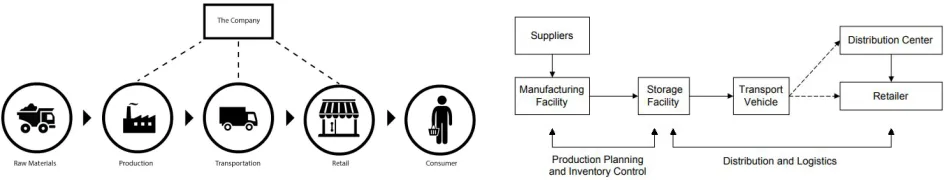
Inventory models are based on a certain demand, either constant or following a series. Future demand is rarely known with certainty. To decrease model complexity, it can be useful to assume the demand pattern is already known (one can for example try to predict future demand using forecasting techniques, or consider a multiple of different scenarios). In this case the mathematical model is assumed to be deterministic. When choosing a stochastic approach, demand, or other factors within the model (e.g. production quantities or lead time) depend on a certain probability distribution. When, for example, a Poisson distribution is used, the chance the demand for a period is at a certain level, corresponds with the chance according to the distribution for that level. In the case of the distribution of figure 7 on the next page for example, there is a fifteen percent chance to reach 1 unit.
[image:13.612.47.547.86.275.2]Figure 7: Probability distribution example (Poisson)
3.6. Optimization Models and Techniques
In an article from Beamon M.B. (1998) summarizing research on supply chain management and optimization, Beamon M.B. states that optimization models can be divided into four categories based on the modelling approach while mentioning relevant articles using the technique. This will gives a good overview which approaches could be suitable for this research. The consideration for the selection of the technique for this research is found in paragraph 4.2.2.
Deterministic Models
As mentioned before, in deterministic models all the variables are assumed to be known. Within the deterministic approach there are different modeling techniques one can use. Williams, J.F. (1981) for example proposed multiple heuristic techniques for scheduling production and distribution. Williams, J.F. (1983) subsequently proposes a dynamic programming algorithm to determine production and distribution sized for an assembly process. Dynamic programming is an approach to solving optimization problems by working backwards. Mixed integer linear programming is another technique that can be used to model a supply chain. This is used for example by Cohen and Lee (1989) who base their model on the EOQ. More recently, a mixed integer linear programming model was proposed by Mohammadi Bidhandi, H. et al (2009) considering multiple commodities and single period.
Stochastic Models
In stochastic models one or more variables are unknown and follow a probability distribution. The same modelling techniques can be used as with a deterministic approach, which includes, but is not limited to, dynamic, linear, non-linear and integer programming models.
Economic Models
The use of economic models is a less often used modeling technique for supply chain design problems. Christy and Grout (1994) use an economic game-theory framework to model relationships between buyers and suppliers within a supply chain. Within game-theory (Morgenstern O. & von Neumann J. - 1944) decisions in certain scenarios are analyzed and tried to be understood.
Simulation Models
Simulation models are mainly used to model an existing supply chain design and test certain strategies for performance. Simulation can be very simple (Monte-Carlo Simulation) or more advanced and detailed (object based discrete event simulation). Towill et al. (1992) has used a simulation model for example to test a just-in-time policy, removing echelons, modifying order quantities and/or procedure parameters. Simulation models can be of deterministic or stochastic nature.
3.7. Demand Forecasting Techniques
demand patterns. Winston W. L. (2004) distinguishes two important methods: extrapolation methods and causal methods:
3.7.1. Extrapolation methods
Within this technique future values of a time series are predicted based on past known values.
Moving average
One of the most widely used and easy forecasting methods is the moving average. The method states that when considering a range of demand with N entries, the next value which is unknown and has to be forecasted is calculated by taking the average of the total value of the N entries. Now the range consists of N + 1 entries. The next value to be forecasted N + 2 will be the average of entries 1 + 1 (=2) to N + 1. Notice the average is ‘moving’.
Exponential smoothing
A more advanced extrapolation method to forecast demand is the exponential smoothing method and its
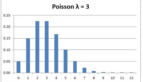
[image:15.612.54.558.266.417.2]extensions. There are three varieties within exponential smoothing, namely simple, double (Holt C.C. - 1957) and triple (Winters P.R. - 1960). When analyzing demand patterns, three properties can often be distinguished: volatility, trend and seasonality.
Figure 8: Volatile demand without trend or seasonality Figure 9: Volatile demand with upward trend
Figure 10: Volatile demand with upward trend and 4 period season
These properties coincide with the three variations on exponential smoothing. Simple exponential smoothing can be used to forecast demand where no trend or seasonality can be detected, like graph in figure 8. This method uses only one smoothing variable α, which can take a value between 0 and 1 and determines how much the volatility of the forecasted demand will be smoothed out (lower peaks, higher lows). Holt's double exponential smoothing should be used instead when the demand line shows an upward or downward trend as depicted in figure 9. This method introduces a second variable β, which can influence the trend of the forecasted values. Lastly, Winters’s triple exponential smoothing is used when there is both trend and seasonality in the demand line
as depicted in figure 10. In this third and final variation a third smoothing variable γ, which influences the degree in
[image:15.612.183.433.457.582.2]3.7.2. Causal forecasting methods
These methods use causality between variables to predict future values. Here the variable which has to be predicted is the dependent variable and the variable used for the prediction is the independent variable.
Regression analysis
Regression analysis may be used to establish if the dependent and independent variable are related and how. Predictions for future values can be based on the mathematical formulation of the relation between the variables. For example, in the case of linear dependence, a linear equation can be formulated and predictions can be based on this equation.
3.8. Forecast Error and Expected Accuracy
Forecasting is never one hundred percent accurate. To measure the degree in which forecasted demand series corresponds to the real demand, a number of techniques can be used. Because whichever forecasting method is used, when this method is used to also forecast known demand, the two series can be compared and the
measure of fit can be determined.
Mean Absolute Deviation
The mean absolute deviation (MAD) shows how much, on average, the forecasted series differs from the known series. This is the absolute average of the forecasted value minus the known value for every period.
Mean Squared Error
The mean squared error (MSE) shows the average of the squared differences of two series of values, often a known series and a predicted series. The MSE is an indicator of the quality of an estimator (the method used to predict a series of data).
Normal Distribution
Winston W.L. (2004) states that with normally distributed forecasting errors it is important to check the accuracy by comparing these values with the normal distribution. Assuming normally distributed errors the standard deviation can be calculated using the formula: standard deviation = 1.25 * MAD. Then, a minimum of 68% of the error values should differ at most one time the standard deviation from the mean and a minimum of 95% should differ at most two times the standard deviation from the mean. If this is not the case the forecast may need extra data, to improve the accuracy of the forecast.
Figure 11: Normal distribution
4. Solution proposition
This chapter will aim to find a suitable technique to substantiate transportation, ordering and inventory quantity decisions. It will elaborate on assumptions made in the mathematical model, and explain the route taken to create the dynamic programming and exponential smoothing model. An overview of the model relations can be found in paragraph 4.5. An overview of the total design process from theory to solution can be found in the conceptual model in appendix B.
4.1. Selection of Technique
4.1.1. Deterministic vs stochastic model
Considering the scope of this research, and it being the first optimization effort within the company, the
deterministic modeling approach has been selected. This way, unnecessary model complexity and development time can be avoided, while the uncertain demand in the multiple period planning scenario can be predicted by demand forecasting. Calculation time will likely be lower as well, which is desirable, since the solution is meant to be used frequently. The model is not meant to be used for a single extensive in-depth recommendation. See also paragraph 4.2.2.
4.1.2. Mathematical Model Selection
Paragraph 3.6 described that within the deterministic modeling approach there are three techniques most
commonly used to solve supply chain inventory problems. These are: (object based discrete event) simulation, linear(integer) programming and dynamic programming. To substantiate the decision for one of these
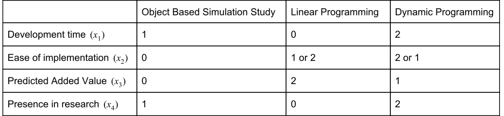
methods, a multi-criteria decision analysis is performed. First, a number of criteria have been defined, ranked by their importance and reviewed. Then, per criterium, the three methods will get 0, 1 or 2 points assigned, indicating how strong the method performs for this criterium. This will be based on both objective and subjective factors. The criteria that will be used for this analysis (with their weight in a percentage) are:
Predicted development time - 35%
This is the prediction of time necessary to construct the (mathematical) model and fashion it in such a way it can be used in the company. This is based on my skill with the approach gained from the IEM program.
Wagner & Whitin (1958) propose to solve the relatively simple dynamic lot-size equation with the dynamic programming technique. This is also the method used in Winston (2004), subsequently followed by the Silver Meal Heuristic which can be used to find a near-optimal solution and involves less work. The work associated with the dynamic programming approach is expected to be easily automated with modern software, so dynamic programming scores highest on this criterium. Development time for a simulation model will depend on the amount of detail and type of simulation. A more extensive object-based discrete-event simulation model (which is the prominent approach within the IEM program), development time is likely higher than a dynamic programming model. The success of a linear programming approach heavily depends on the construction of constraints. Certain aspects that would need to be included for sufficient correspondence with reality (i.e.: future demand over multiple periods) would extend beyond the material from the IEM program. Therefore, linear programming scores lowest on this criterium.
Implementation in company - 35%
This is a combination of the time the company needs to use or implement the solution and how easily the solution can be integrated in the current process without the need of additional personnel etc.
One of the advantages of linear programming is the amount of detail that can be added to the model. Letting transportation decisions depend on production decisions can, for example, be combined in a single model and will provide the company with a really extensive solution. Ease of implementation of both linear and dynamic
existing process. The most important bottlenecks are already known however, and high cost investments are not being considered at the moment of writing this report.
Predicted added value - 20%
This is the added value the solution is likely to bring the company compared to the current process and for their current situation and size.
The company is in a beginning stage of redesigning and optimizing their supply chain processes. Reasons to opt for a simulation approach (i.e.: high cost investments, interactions of components, testing of strategies) are therefore not yet present, so this technique scores lowest. On the other hand, mathematical insight into inventory management might not only help determine order- and transportation quantities for combined demand of multiple clients, but also help determine next steps in this area. Linear programming has the highest possibility for very extensive and in-depth model and scores therefore highest.
Presence in existing research - 10%
This is based on the number of articles that already use the approach according to the SLR (chapter 3.1).
Optimal order and transportation quantities can be calculated with either dynamic or linear programming. The linear programming approach is the most used approach in the articles reviewed in the SLR, while no articles use dynamic programming. Using an approach which is new in the existing research field may provide interesting possibilities (better implementation possibilities in a small company) and/or insights, so LP scores lowest and DP highest.
Object Based Simulation Study Linear Programming Dynamic Programming
Development time (x1) 1 0 2
Ease of implementation (x2) 0 1 or 2 2 or 1
Predicted Added Value (x3) 0 2 1
[image:18.612.50.569.312.432.2]Presence in research (x4) 1 0 2
Table 1: Multi-Criteria Decision Analysis score table
MCDA formula:
ax q 0.35x 0.35x 0.2x 0.1x
M = 1 + 2 + 3 + 4
Within the calculation favoring dynamic programming the object based simulation study scores 0.45 points, linear programming 0.75 point and the dynamic programming approach 1.8 points. When switching x2 in favour of LP, it scores 1.1 points and DP 1.45 points. Therefore, deterministic dynamic programming will be used in this research.
4.1.3. Selection Forecasting Model
To provide the model with deterministic demand the triple exponential smoothing (TES) forecasting technique is selected. This technique is one of the more extensive extrapolation forecasting methods and is generally
4.2. Assumptions and Limitations of the Models
Within the dynamic programming, and forecasting models, several assumptions have been made. These will be presented below.
4.2.1. Assumptions for the Supply Chain
1. The supply chain where the model is applicable consists of a single supplier and multiple customers. 2. The model will determine optimal inventory decisions, so vehicle routing is excluded. This is not the
responsibility of the company.
3. Product X is bought at the producer in a certain quantity of whole pallets.
4. Production is assumed to take one week and consequently enters the inventory of the company at the production plant.
5. When deciding to transport a certain number of pallets, these are shipped from Italy to multiple customers in northern Europe via the transportation company, who receive a transport order.
6. Transported product can also be added to inventory in the Netherlands or possibly delivered early to a customer.
4.2.2. Demand
Demand will be assumed to be deterministic. At this moment there is no need to make the model more
complicated using stochastic modeling, and most likely significantly improve the calculation speed. Per period of the planning horizon the demand represents the total amount of product X that has to be delivered to customers. Backlogging is not allowed, as the company risks big penalties for late delivery. One of which could be losing the account. Because demand is assumed to be known, which is not always the case, the dynamic program is extended with a triple exponential smoothing forecasting algorithm to predict as accurately as possible the demand for the planning horizon.
4.2.3. Assumptions for the ordering quantity dynamic program
The ordering quantity cost function from paragraph 4.3. is subject to the following assumptions:
1. The length of one period is assumed to be two weeks to provide a clearer resemblance to reality for the company. This does not have an impact on results and the mathematical formula, but will increase credibility. These two weeks consist of 1 week production time and 1 week transportation to satisfy demand at the end of the period.
2. This model uses the output of the transportation quantity model to calculate the ordering quantity per period.
3. The ‘holding cost’ is calculated as a percentage of production order value. This is done for two reasons: firstly, since the producer is shareholder, the company does not pay to store pallets of product X at the production location, so direct holding costs cannot be used. Therefore, the risk of investment in product is regarded as holding cost. Secondly, as mentioned before, when more of the same product is produced, the company can make use of quantity discounts at the producer. Quantity discounts mean a smaller total investment per unit of product and a smaller investment risk.
4. For every production order, an order cost can be assigned, this can reflect reality (salary of employee who orders the product) or used to influence results and test different scenarios. Also starting inventories can be set.
5. Inventory is assumed to be 0 at the end of the planning period.
4.2.4. Assumptions for the Transportation Quantity Dynamic Program
The transportation quantity cost function from paragraph 4.3. is subject to the following assumptions:
1. The cost function of the transportation quantity dynamic program uses the same structure as the ordering quantity model. In this model, based on forecasted demand, the model will calculate transportation quantities that minimize total transportation costs. So in this model, the production quantity discounts from the previous model will be regarded as the transportation cost for n pallets which also decreases in a price discounted fashion.
3. Maximum ordering cost will be regarded as maximum transportation quantity or vehicle capacity. 4. Holding cost is regarded as the cost to keep inventory in the Netherlands or to regulate the amount of
product that can be delivered early to the customer. Storage capacity in the Netherlands is already available via a partner.
5. No vehicle routing is considered, as this is the responsibility of the transportation company. 6. Inventory at the end of the planning period is assumed to be 0.
4.2.5. Factors of the Forecasting Model
Certain steps have been taken to evaluate the probable accuracy of the calculated forecast in the model, based on the highlighted techniques of section 3.7. Based on the error values when comparing the forecast with the known demand, the MSQ, MAD and SD are calculated to give an impression of accuracy. Besides this, the distribution of the error values will be compared to the normal distribution with the same mean and standard deviation.
4.3. Dynamic Programming Model
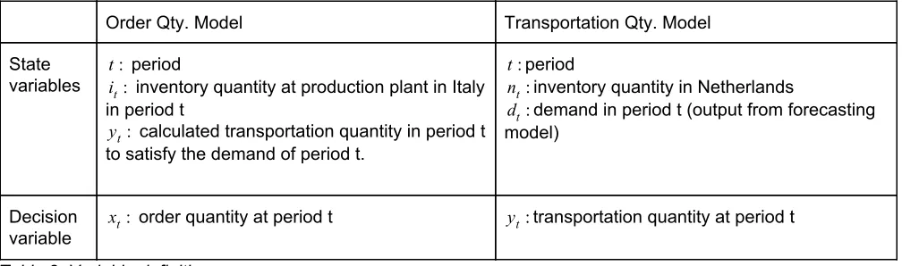
The dynamic programming model needs to determine transportation and ordering quantities that minimize costs over a planning horizon. Therefore, the model is separated into two models. Both these models aim to minimize a total cost function based on the dynamic lot-size model. Table 2 below gives an overview of the definitions of variables in the cost function ft(i), where one unit of product X corresponds with one pallet. ft(i) dictates the minimum cost achievable in period t when i units product are in inventory.
Order Qty. Model Transportation Qty. Model
State variables
period t:
inventory quantity at production plant in Italy it:
in period t
calculated transportation quantity in period t yt:
to satisfy the demand of period t.
period t:
inventory quantity in Netherlands nt:
demand in period t (output from forecasting dt:
model)
Decision variable
order quantity at period t
[image:20.612.55.559.299.448.2]xt: yt:transportation quantity at period t
Table 2: Variable definitions
Definition of the cost functions:
(i) min {(h c(x) (i x y)) ((c(x) x) o) f (i x )} ft = * t * t + t − t + t * t + + t + 1 t + t −yt
(n) min {(h c(y) (n y d)) ((c(y) y) o) f (n y )} ft = * t * t + t − t + t * t + + t + 1 t + t −dt
Subject to:
xt , yt , it , nt , dt ≥ 0
Input values:
: investment risk and opportunity cost when investing in inventory at production plant (ordering model) or at a h
warehouse in the Netherlands (transportation model) as a percentage of c(x).
(ordering model): investment cost in 1 unit product when ordering x units product. (x)
c
(transportation model): investment cost in transportation of 1 unit product when transporting x units product. (x)
c
: fixed cost of sending a production or transportation order. o
product or both. The cost associated with fulfilling demand for every level of inventory and ordering/transportation quantity is then calculated first for the last period of the planning horizon. Then, this process is repeated for every remaining period working backwards adding the minimum cost of the previously calculated period. How this model will be calculated efficiently and easy to implement in the company will be discussed in paragraph 4.5.
4.4. Triple Exponential Smoothing Model
Triple exponential smoothing (TES) is a mathematical technique to forecast demand patterns. This model
accounts for a combination of volatility, trend and seasonality factors. TES predicts a demand value for one period in the future based on a number of values which are calculated and updated on the basis of known demand p)
(
. Different variables are used in this model, because in this model historical demand is used, whereas in the Yp
dynamic programming models, demand is based on the prediction of this model. Every period gets three values assigned to it:
1. A level value L which indicates the basis value to calculate the demand prediction. 2. A trend value T, which indicates the slope of the demand.
3. A seasonal value S, which indicates how every period in a season behaves according to seasonal factors.
The amount to which these values impact the predicted value Fp, is influenced by the smoothing parameters ⍺, 𝛽 and 𝛾. These parameters can range between 0 and 1, to have either a small or large effect.
4.4.1. Standard TES formulas
The standard formulas can be found in Appendix C
4.4.2. Example calculations, forecast error and forecast accuracy
An example of calculations made to predict a future demand pattern as is done in the Excel tool can be found in Appendix D.
Because predictions are also made for the periods where demand is already known, the accuracy of the forecast is assessed by analyzing the error values. For this research the mean square error (MSE) and the mean absolute deviation (MAD) have been used:
AD
M = 24
Y − F ∑
24
p = 1| p p|
SE
M = 24
(Y − F )
∑
24
p = 1 p p
2
Minimizing the total error can provide values for α , β and for which the forecast is most accurate. This will beγ further explored in the next chapter, as well as the comparison to the normal distribution proposed by Winston W.L. (2004) and the calculation of the standard deviation.
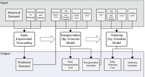
[image:21.612.153.461.575.739.2]4.5. Overview of Input and Output Streams
4.6. Implementation of Solution
As was stated in paragraph 3.1. the solution should be easily implementable, usable and understandable by the company. This is one of the reasons why the dynamic programming approach with deterministic demand is used. This approach is relatively simple and can be programmed in visual basic for applications (VBA, a programming language of Microsoft Excel) within the time constraints. Excel is used so the company does not need extra software, knowledge or time to use the solution and has a fast and clear overview of the output of the model. The KPI that can be used is the total transportation cost as a percentage of company revenue. In the forecasting model the KPI that is used to assess the quality of the forecast is the mean squared error.
5. VBA Tool
This chapter will give an overview of the decisions made to program the mathematical model in VBA. An
explanation on how the tool functions will be given and the model will be validated. At the end of this chapter it will be explained how the program can contribute in the daily decision processes of the company
5.1. VBA Programming Approach
This paragraph will describe the decisions made to program the mathematical program in VBA (Visual Basic for Applications). A step by step description of the VBA code with explanatory text (in green) can be found in Appendix E. The method described in Winston W.L. (2004) to solve dynamic lot-size inventory problems is used as a general guideline. The first step is to calculate the costs for the last period, where the number of periods, maximum inventory amount, maximum production amount, inventory costs, ordering cost, starting inventory, (price discounted) investment cost and demand are all variable and can be influenced in the input section of the dashboard. The total cost for every combination of possible inventory levels and ordering amount per period is assigned to a three-dimensional array F(period, inventory level, production level). Every time this is done, it is checked if this total cost value is lower than the current optimal value F, if this is the case this becomes the new value for F for the corresponding period and inventory level. The optimal production level is assigned to the array X. The final optimal values are outputted to their cells in the dashboard for the production schedule.
The standard ordering quantity dynamic program does not account for transportation time. When the way of thinking when solving dynamic programs is used however, the two dynamic programs can be combined. The demand can be used normally as input for the transportation planning model. The output of the transportation planning can then be used as input for the order planning model. In VBA, the code for the transportation quantity model is the same as the ordering quantity model. In the case of deterministic demand, the amount of pallets that have to be delivered, so transported from the production facility to the client, is known. When this is known, the amount has to be ready (produced) on time is known as well. This can be used as input for the ordering quantity model.
Within the triple exponential smoothing model VBA program, multiple arrays are used to store the calculated values of Yp(historical demand), Lp (level value), Tp (trend value), Sp (seasonal value) and Fp (forecasted value) which correspond with these letters. The values for α , β, γ (smoothing parameters), the number of known periods and the number of periods to predict can be adjusted in the dashboard and are assigned to VBA
variables.
The initial values for Sp = 1 to Sp = season, Lp = 1, Tp = 1 and Sp = season + 1 are calculated using the formulas from Holt C.C. (1957). These values can be used to calculate the first value for Fp = season + 2. Then, for the next number of periods the values of Lp, Tp and Sp can be updated per known period and Fp + 1 can be calculated for these periods. One season before the last period, Sp cannot be updated anymore and last-known values must be used. To calculate the values Fpfor the forecast period, the parameter is used, which increases by 1 for every nextk period to influence the trend value. Next, the error values (MSE, MAD) are calculated and assigned to a new array which are outputted to the dashboard.
5.2. Program dashboard functions and usability
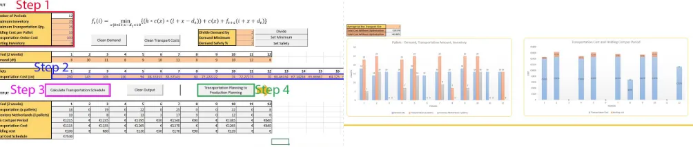
This paragraph will shortly explain how these dashboards can be used to get to an optimal transportation and ordering schedule. An overview of the Excel dashboards can be found in figure 13, 14, 15, 16 where the 4 steps are highlighted. The three complete dashboards can be found in appendix F
5.2.1. Forecast Dashboard
Step 1 - Input known demand
First input demand that is known. It does not matter how many periods or which unit of demand measurement is used (for this example pallets are used), however more periods of known demand will give a more accurate forecast. Also for TES to work properly, there should at least be three complete seasons of known data available.
Step 2 - Input necessary variables
Now the necessary variables for TES have to be inputted. When the number of periods per season are unknown, the graph on the right of the input section can be consulted, since the demand will automatically update in this graph. A longer forecast period will be less accurate than a shorter one obviously. α , β and input can be setγ manually or step three can be used to calculate the optimal values. When extra accuracy for α , β and isγ needed the number of decimals can be increased, but the calculation optimal values will be slower.
Step 3 - Calculate the forecast
When everything is set in the input section, the demand can be forecasted. On the right in the output section the forecasted values and error values will be outputted. The graph showing the known demand and forecasted demand will be updated, as well as a graph showing the number of certain error values, and how well they compare with the normal distribution with corresponding mean and standard deviation.
Step 4 - Use the forecasted values as input for the transportation model
[image:23.612.63.225.413.635.2]This button can be used to easily copy the forecasted values to the next step and switch sheets to calculate the optimal transportation schedule.
[image:23.612.264.566.418.625.2]5.2.2. Transportation Schedule
Step 1 - Input the necessary variables
First the input variables can be adjusted, such as maxima for inventory or transportation quantity. Each time a transportation order is sent, a fixed cost can be assigned (such as employee salary, or to influence the calculation). Also, if there is still inventory left from an earlier calculation this can be included.
Step 2 - Input transportation cost
Because the demand is already copied from the previous sheet, only the cost of transporting a number of pallets has to be set, this is the cost per pallet of transporting that number of pallets.
Step 3 - Calculate schedule
The next step is to calculate the schedule for the inputted values with which the cost function is minimized. The schedule and associated costs will be outputted to the table below and the two graphs.
Step 4 - Use output on next sheet
[image:24.612.63.565.275.382.2]To use the transportation schedule as input for the production schedule this button can be used to automatically copy the values.
Figure 15: Transportation quantity dashboard - Figure 16: Accompanying graphs
5.2.3. Ordering Schedule
Step 1 - Input the necessary variables
Again, the input variables can be adjusted, such as maxima for inventory or ordering quantity. Each time a production order is sent, a fixed cost can be assigned (such as employee salary, or to influence the calculation). Also, if there is still inventory left from an earlier calculation this can be included.
Step 2 - Input product cost
The transportation schedule is already copied from the previous sheet, and serves as demand in this model. Only the cost of a certain number of pallets of product X has to be set, this is the cost per pallet of when buying that number of pallets.
Step 3 - Calculate schedule
Figure 17: Ordering Schedule
5.5. Validation ordering and transportation quantity model
The ordering/transportation model can be validated by inserting a known scenario. In this case, since the technique from Winston W.L. (2004) is used to solve an inventory problem, the example scenario can also be used to validate the model.
In this example, there are four periods, where demand follows the following pattern:
Period 1: 1 Period 2: 3 Period 3: 2 Period 4: 4
The setup cost equals €3, production cost per unit equals €1 and holding cost equals €0.50 per unit. The maximum production level is 5 units and maximum inventory is 4 units.
Using these values as input for the model, the following output is calculated:
Figure 18: Production schedule output using known situation
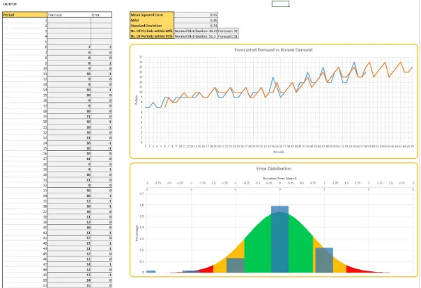
[image:25.612.60.348.479.556.2]5.6. Validation Forecasting Model
Figure 19: Example Forecast output
Every time the forecast is performed the quality of the forecast can be assessed. Error values are calculated per known period, with which the mean squared error, the mean absolute deviation and the standard deviation for these errors is calculated. According to Winston W. L. (2004) it can be assumed that forecast errors are normally distributed. Therefore, the calculated errors are compared with the normal distribution. Also it becomes clear how much error values differentiate either more than one or more than two standard deviation from the mean.
5.7. Implementation of Excel Tool
The proposed solution has taken into account easy implementation in the company. How this solution can fit into the current process will be outlined in this paragraph.
Based on historical demand of the company a forecast can be made for the upcoming t periods. This historical demand may have to be adjusted for the period length of 2 weeks. The forecasted demand can then quickly be inserted in the transportation planning sheet. In this sheet the predicted demand may be adjusted slightly to include a safety percentage, or already known orders. Then, using the right input values, an optimal transportation schedule can be calculated for the predicted demand. This schedule can be used to put in transportation orders in advance, or as a basis for more general strategy decisions. In certain situations it may, for example, be more cost efficient to transport a number of pallets equal to 4 or 6 weeks of demand and keep this in stock. The next step, an optimal production schedule can be calculated using the transportation schedule and meet the required transportation amounts. This schedule can be used to let the production plant know when to expect orders of a certain size, or substantiate broader production quantity strategy.
Because the program works in Excel, it is expected to be quickly understood and usable for the company. Demand analysis and tracking is already done in Excel, and this data can easily be copied in the program since it takes data from Excel worksheets and not a user form. Adjustments to predictions or calculations can easily be done and the whole process, from historical demand to production schedule, takes less than 5 minutes and only has to be done once every few weeks.
6. Evaluation
The evaluation of the proposed solution will look at two areas: usability of the model and the output of the tool.
6.1. Usability
One of the most important criteria the solution had to meet was easy and fast implementability and simplicity of use. When the tool was presented to the CEO of the company, who mainly has expertise in sales and
management, the tool could be explained in about twenty minutes. This explanation included usability, the principles of dynamic programming and forecasting and how the tool would calculate a solution which would be more optimal than the current process. The limitations and use case scenarios were covered as well.
Also, because only Excel is needed to run the tool (which is already used by the company) it allows for easy and fast implementation with a separate extended guide. The fact that calculations take a really short amount of time and at most 4 steps are needed to get results adds to the usability of the solution. Some calculation times in different scenarios are presented in table 3:
Forecast Smoothing Var. Transportation Ordering
64 periods 1 decimals
12 period forecast
0.85 s 0.21 s 12 periods
97 demand
0.12 s 0.11 s
64 periods 1 decimals
24 period forecast
0.75 s 0.22 s 12 periods 194 demand
0.14 s 0.12 s
64 periods 2 decimals
12 period forecast
0.88 s 170.65 s 24 periods 194 demand
0.17 s 0.12 s
32 periods 2 decimals 24period forecast
[image:27.612.54.554.240.457.2]0.89 103.7 s
Table 3: Calculation time of different scenarios
6.2. Realization of the norm
Figure 20: Transportation Price Discount (data from transportation company)
A substantial cost reduction may be obtained in case an alternative to the ad hoc policy is used. Below is an example using the most frequent average transportation sizes used by the company. These average transport batch sizes are assumed following this logic: from the product X variety with the highest revenue 48 pallets were sold in 2018. This means 24 pallets in half a year. When using periods of 2 weeks on average a minimum of 2 pallets is sold (transported) every two weeks. This value is likely to be slightly higher because of individual orders from clients are not received every two weeks. Therefore this value is assumed to be an average of 3, but also 2 and 4 are included for comparison.
Figure 21: Expected transportation cost reductions
This is, as expected, a significant cost reduction. This however is an approximation, since this does not include priority transportation cost, or other measures that can drive up total transportation cost when no stock is kept. When these reductions are compared to the norm of 3 percent of the revenue, it can be concluded that this could be reached using this tool. For the demand pattern corresponding to the ‘average ad hoc transport size’ of 4, which utilizes the price discount the most and is therefore the most efficient, the model will produce a
transportation cost of about 3.2 % of the revenue. When an average transport batch size of 3 pallets is assumed the model will reduce cost by 61.73 % which corresponds to 1.3 % of the total revenue defined earlier.
[image:28.612.241.372.301.330.2]Looking at the ordering schedule Excel tab, the transportation planning of the previous part and a linearly decreasing quantity discount is used as input. Below are some resulting cost reduction percentages.