Teacher and school effects on student achievement

(1)

warwick.ac.uk/lib-publications

A Thesis Submitted for the Degree of PhD at the University of Warwick

Permanent WRAP URL:

http://wrap.warwick.ac.uk/81768

Copyright and reuse:

This thesis is made available online and is protected by original copyright. Please scroll down to view the document itself.

Please refer to the repository record for this item for information to help you to cite it. Our policy information is available from the repository home page.

(2)

Teacher and school effects on student

achievement

by

Mario Fernando Sanclemente Villegas

Thesis

Submitted to the University of Warwick for the degree of

Doctor of Philosophy

Department of Economics

(3)

List of Tables

1.1 Educational levels and pupils’ age . . . 2

2.1 Standard Deviations of Teacher effects estimates in the literature . 51 3.1 Usage of performance data bases by chapters and cohorts . . . 56

3.2 Variables Description - Individual Scores DB . . . 64

3.3 Variables Description - Directories DB . . . 65

3.4 Variables Description - Parental Questionnaire DB . . . 65

3.5 Variables Availability - Parental Questionnaire DB . . . 65

3.6 Number of Students by year and grade . . . 66

3.7 Number and distribution of students by type of dependence . . . . 67

3.8 Number and distribution of schools by type of dependence . . . 67

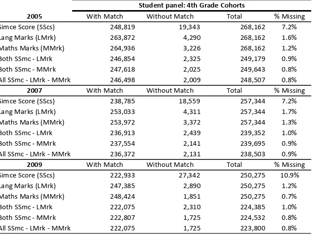
3.9 Match between performance data bases (selected cohorts) . . . 70

3.10 General correlations - Selected cohorts . . . 71

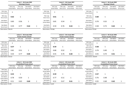
3.11 Correlation matrices by type of school dependence - 4th _{grade cohorts 71} 3.12 Correlation matrices by rurality - 4th _{grade cohorts . . . 72}

3.13 Linear regressions (4th grade cohorts 2005-2007-2009) . . . 76

4.1 Reduced panels for selected cohorts . . . 82

4.2 Selected cohorts transition . . . 82

4.3 Matching school marks to students in selected cohorts . . . 83

4.4 Matching teachers to classrooms by subject in selected cohorts . . . 84

4.5 Teacher classification at student level in selected cohorts . . . 84

4.6 Teacher classification at class level in selected cohorts . . . 85

4.7 Summary statistics mini panel Cohort 1 . . . 86

4.8 Distribution of schools by number of classes per grade (Mini panel Cohort 1) . . . 87

4.9 First criterion: School selection . . . 87

(8)

4.13 Student mobility in the mini panel . . . 89 4.14 Summary statistics mini panel Cohort 1 - Groups 1 & 2 . . . 91 4.15 Distribution of students by type of school dependence in mini panel

Cohort 1 - Groups 1 & 2 . . . 92 4.16 Non-random assignment (Non-RA) Indexes per school . . . 102 4.17 Potential cases of non-random assignment tested with RDM

coun-terfactuals (Group 1) . . . 102 4.18 Potential cases of non-random assignment tested with RDM

coun-terfactuals (Group 2) . . . 103 4.19 Potential cases of non-random assignment tested with SRT

coun-terfactuals (Group 1) . . . 104 4.20 Potential cases of non-random assignment tested with SRT

coun-terfactuals (Group 2) . . . 105 4.21 Estimated levels of Non-Random assignment (Group 1) . . . 107 4.22 Estimated levels of Non-Random assignment in percentage (Group

1) . . . 107 4.23 Estimated levels of Non-Random assignment (Group 2) . . . 108 4.24 Estimated levels of Non-Random assignment in percentage (Group

2) . . . 108 4.25 Estimated levels of Non-Random assignment in percentage (Groups

1 & 2) . . . 109 5.1 Sample Selection Criteria - 2005 4th _{grade cohort} _{. . . 123}

5.2 Number of observations dropped by type of selection . . . 124 5.3 Descriptive statistics - Before and after selection (4th _{grade cohort}

2005) . . . 125 5.4 Maximum Likelihood coefficient estimates - 4th grade 2005 selected

sample cohort . . . 127 5.5 Simce scores distribution - 4th _{grade 2005 selected sample cohort . . 131}

5.6 Distribution of Teacher Effects, Hypothetical Treatment and Teacher Ranking - 4th _{grade 2005 selected sample cohort . . . 133}

5.7 Descriptive statistics single-sex schools - 4th _{grade 2005 selected}

sample cohort . . . 136 5.8 Simce score distribution by gender-type of school - 4th _{grade 2005}

selected sample cohort . . . 137 5.9 Distribution of Teacher Effects, Hypothetical Treatment and Teacher

(9)

5.10 Descriptive statistics by type of school dependence - 4th _{grade 2005}

selected sample cohort . . . 142

5.11 Simce score distribution by type of school dependence - 4th _grade 2005 selected sample cohort . . . 143

5.12 Distribution of Teacher Effects, Hypothetical Treatment and Teacher Ranking - 4th _{grade 2005 selected sample cohort by type of school} dependence . . . 145

6.1 Sample selection criteria - 4th grade cohorts (2005 - 2009) . . . 162

6.2 Number of observations dropped by type of selection - 4th grade cohorts (2005-2009) . . . 164

6.3 Maximum Likelihood coefficient estimates - 4th _{grade selected} sam-ple cohorts 2005-2009 . . . 166

6.4 Observed patterns in original school panel . . . 171

6.5 Observed patterns in the reduced school panel . . . 172

6.6 Number of schools shifting to subject specialist (SS) teacher scheme 173 6.7 Descriptive statistics: Original vs Reduced School Panel - 4thgrade cohorts: 2005-2009 . . . 174

6.8 Transition matrices . . . 175

6.9 Transition matrices (percentage) . . . 176

6.10 Set of conditions - Downward trajectory schools . . . 177

6.11 Set of conditions - Upward trajectory schools . . . 177

6.12 Distribution of trajectories by trackable groups . . . 178

6.13 Changes to subject specialist (SS) teacher scheme by trajectory groups . . . 178

6.14 Descriptive statistics: Type of quality trajectory - 4thgrade cohorts: 2005 - 2009 . . . 181

8.1 Summary of Data Sets in the VAM Literature . . . 202

8.2 Summary Statistics - Cohort 2 . . . 211

8.3 Summary Statistics - Cohort 3 . . . 212

8.4 Estimated levels of Non-Random assignment - Group 1 & 2 (Cohort 2) . . . 221

8.5 Estimated levels of Non-Random assignment in percentage - Group 1 & 2 (Cohort 2) . . . 221

8.6 Estimated levels of Non-Random assignment - Group 1 & 2 (Cohort 3) . . . 222

(10)

8.8 Maximum Likelihood coefficient estimates by gender-type of school

- 4th _{grade 2005 selected sample cohort . . . 224}

8.9 Maximum Likelihood coefficient estimates by type of school depen-dence - 4th _{grade 2005 selected sample cohort} _{. . . 225}

8.10 Simce distribution - Absolute and standardised Simce scores - 4th grade 2005 selected sample . . . 226

8.11 Empirical Bayes distributions - All schools - 4th grade 2005 selected sample . . . 228

8.12 Empirical Bayes distributions - Girls-only schools - 4th grade 2005 selected sample . . . 229

8.13 Empirical Bayes distributions - Boys-only schools - 4th _{grade 2005} selected sample . . . 230

8.14 Empirical Bayes distributions - Municipal & Private Voucher schools - 4th _{grade 2005 selected sample . . . 231}

8.15 Empirical Bayes distributions - Municipal schools - 4th _{grade 2005} selected sample . . . 232

8.16 4th grade cohort 2005 - Before and after selection . . . 233

8.19 4th _{grade cohort 2008 - Before and after selection} _{. . . 236}

8.20 4th _{grade cohort 2009 - Before and after selection} _{. . . 237}

8.21 Simce score distribution - 4th _{Grade cohorts (2005 - 2009) . . . 238}

8.22 Estimated Teacher Effects and Hypothetical Treatment - Selected sample cohorts (4th _{grade 2005-2009) . . . 238}

8.23 Estimated of School Effects and Hypothetical Treatment - Selected sample cohorts (4th grade 2005-2009) . . . 239

8.24 Empirical Bayes distributions - 4th grade 2005 selected sample . . . 240

8.25 Empirical Bayes distributions - 4th grade 2006 selected sample . . . 241

8.26 Empirical Bayes distributions - 4th _{grade 2007 selected sample . . . 242}

8.29 Cross Section cohorts 4th _{Grade 2005 - 2009 . . . 252}

8.30 Transition matrices - Groups 1.1 & 1.2 . . . 253

(11)

List of Figures

3.1 Processing Data Sets - Flowchart . . . 59

3.2 Timeline - Simce . . . 68

3.3 Selected cohorts . . . 69

3.4 Stdsed. School Marks vs Stdsed. Simce Scores (4th _{grade cohorts} 2005-2007-2009) . . . 73

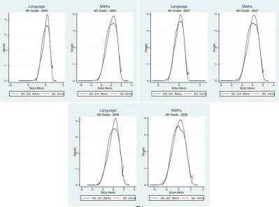
3.5 Kernel distributions in Municipal schools (4th _{grade cohorts} 2005-2007-2009) . . . 74

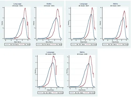
3.6 Kernel distributions in Private Voucher schools (4th grade cohorts 2005-2007-2009) . . . 74

3.7 Kernel distributions in Unsubsidised Private schools ( 4th _grade cohorts 2005-2007-2009) . . . 75

4.1 Class Size Histogram in selected groups . . . 90

4.2 Counterfactual classes generating process - Group 1 . . . 93

4.3 Counterfactual classes generating process - Group 2 . . . 94

4.4 Real classes vs random counterfactuals based on GPA (Group 1) . . 95

4.5 Real classes vs random counterfactuals based on GPA (Group 2) . . 96

4.6 Real classes vs perfectly sorted counterfactuals based on GPA (Group 1) . . . 97

4.7 Real classes vs perfectly sorted counterfactuals based on GPA (Group 2) . . . 97

4.8 Real classes vs random counterfactuals based previous school marks (Group 1) . . . 99

4.9 Real classes vs random counterfactuals based previous school marks (Group 2) . . . 99

4.10 Real classes vs perfectly sorted counterfactuals based previous school marks (Group 1) . . . 100

4.11 Real classes vs perfectly sorted counterfactuals based previous school marks (Group 2) . . . 100

(12)

5.2 Path diagram for teacher effects estimation . . . 118

5.3 Kernel distributions: Stdsed. Simce Scores - Before and After Se-lection (4th _{grade cohort 2005) . . . 125}

5.4 Empirical Bayes distribution of Teacher Effects - 4th _{grade 2005} selected sample cohort . . . 131

5.5 Kernel distributions: Stdsed. Simce Scores single-sex schools - 4th grade 2005 selected sample cohort . . . 136

5.6 Empirical Bayes distribution of Teacher Effects by gender-type of school - 4th grade 2005 selected sample cohort . . . 138

5.7 Empirical Bayes distribution of Teacher Effects within girls-only schools - 4th _{grade 2005 selected sample cohort . . . 139}

5.8 Kernel distributions: Stdsed. Simce Scores by type of school de-pendence - 4th _{grade 2005 selected sample cohort} _{. . . 142}

5.9 Empirical Bayes distribution of Teacher Effects by type of school dependence - 4th _{grade 2005 selected sample cohort . . . 144}

5.10 Empirical Bayes distribution of Teacher Effects within Municipal schools - 4th grade 2005 selected sample cohort . . . 144

5.11 Empirical Bayes distribution of Teacher Effects separated by type of school - 4th grade 2005 selected sample cohort . . . 146

6.1 Type of teacher specialisation 2005 - 2009 . . . 169

6.2 Type of teacher quality 2005 - 2009 . . . 170

6.3 School rankings 2005 - 2009 . . . 179

6.4 School effects evolution 2005 - 2009 . . . 183

6.5 School effects evolution 2005 - 2009 - With and without subject specialist (SS) teacher scheme . . . 184

6.6 School trajectory 2005 - 2009 by type of school dependence . . . 184

6.7 Teacher specialisation evolution 2005 - 2009 by school quality tra-jectory . . . 186

6.8 Teacher quality evolution 2005 - 2009 by school quality trajectory . 188 8.1 Real classes vs random counterfactuals based on GPA - Group 1 (Cohort 2) . . . 213

8.2 Real classes vs random counterfactuals based on GPA - Group 2 (Cohort 2) . . . 213

8.3 Real classes vs perfectly sorted counterfactuals based on GPA -Group 1 (Cohort 2) . . . 214

(13)

8.5 Real classes vs random counterfactuals based previous school marks Group 1 (Cohort 2) . . . 215 8.6 Real classes vs random counterfactuals based previous school marks

Group 2 (Cohort 2) . . . 215 8.7 Real classes vs perfectly sorted counterfactuals based previous school

marks Group 1 (Cohort 2) . . . 216 8.8 Real classes vs perfectly sorted counterfactuals based previous school

marks Group 2 (Cohort 2) . . . 216 8.9 Real classes vs random counterfactuals based on GPA - Group 1

(Cohort 3) . . . 217 8.10 Real classes vs random counterfactuals based on GPA - Group 2

(Cohort 3) . . . 217 8.11 Real classes vs perfectly sorted counterfactuals based on GPA

-Group 1 (Cohort 3) . . . 218 8.12 Real classes vs perfectly sorted counterfactuals based on GPA

-Group 2 (Cohort 3) . . . 218 8.13 Real classes vs random counterfactuals based previous school marks

Group 1 (Cohort 2) . . . 219 8.14 Real classes vs random counterfactuals based previous school marks

Group 2 (Cohort 3) . . . 219 8.15 Real classes vs perfectly sorted counterfactuals based previous school

marks Group 1 (Cohort 3) . . . 220 8.16 Real classes vs perfectly sorted counterfactuals based previous school

marks Group 3 (Cohort 3) . . . 220 8.17 Empirical Bayes distribution of Student Ability - 4th _{grade 2005}

selected sample cohort . . . 223 8.18 Empirical Bayes distribution of Teacher Effects - 4th grade 2005

selected sample cohort . . . 223 8.19 Empirical Bayes distribution of School Effects - 4th _{grade 2005}

se-lected sample cohort . . . 223 8.20 Kernel distributions: Stdsed. Simce Scores - Before and After

Se-lection - 4th _{grade cohort 2005 . . . 233}

8.21 Kernel distributions: Stdsed. Simce Scores - Before and After Se-lection - 4th _{grade cohort 2006 . . . 234}

8.22 Kernel distributions: Stdsed. Simce Scores - Before and After Se-lection - 4th grade cohort 2007 . . . 235 8.23 Kernel distributions: Stdsed. Simce Scores - Before and After

(14)

8.24 Kernel distributions: Stdsed. Simce Scores - Before and After Se-lection - 4th _{grade cohort 2009 . . . 237}

8.25 Disaggregated type of teacher specialisation 2005 - 2009 . . . 245 8.26 Aggregated type of teacher specialisation (2005-2009) - Municipal

schools . . . 246 8.27 Aggregated type of teacher specialisation (2005-2009) - Private Voucher

schools . . . 247 8.28 Aggregated teacher specialisation (2005-2009) - Unsubsidised

Pri-vate schools . . . 248 8.29 Disaggregated teacher specialisation histogram (2005-2009) by teacher

quality . . . 249 8.30 Disaggregated teacher specialisation distribution (2005-2009) by teacher

quality . . . 250 8.31 Disaggregated teacher specialisation evolution (2005-2009) by school

(15)

Acknowledgments

I have no words to express my gratitude to my supervisors Professor Wiji

Aru-lampalam andProfessor Robin Naylor. I feel very lucky of having the opportunity

to live this life experience close to them. With them I have received the best academic training and research orientation. They have always encourage and sup-port me unconditionally, sharing with me their knowledge and time with extreme generosity.

Thanks to the Warwick Economics Department, particularly to Dr Roland

Rathelot, Dr Clement de Chaisemartin, and many others who gave me helpful

comments in the CAGE-AMES Seminars and were willing to meet me and giving me their advice. Thanks to my friends at Warwick, they were my family here and made more enjoyable this process. I would especially want to thank to Mrs

Margaret Nash for being always worried about us and keeping our days sweet and

happy.

Thanks to my family; my parentsFernando andMaria Cristina, my brother

Daniel, and my sisterXimena, because despite of the distance and time, they have

always made me feel as if I have never left home. Thanks to my girlfriend, and future wife Maria Teresa, for helping me to achieve this dream.

Thanks to the Chilean Government for the financial support, provided by means of the CONICYT BECAS CHILE Folio 72100370.

(16)

Declarations

I declare that the contents of this thesis are based on my own research in ac-cordance with the regulations of Warwick University. The work in this thesis is original, unless where indicated by references. This thesis has not been submitted for examination at any other university.

(17)

Abstract

This thesis investigates the topics related to the estimation of Teacher Ef-fectiveness (TEs) and School EfEf-fectiveness (SEs). With regard to TEs, the focus is on the predicted teacher impact on improving academic achievement when a student from the median (or the mean) of the achievement distribution is exposed to a more effective teacher. Regarding SE estimates, we explore the evolution of SEs over a specific period of time. In both cases, we base our estimations on the Chilean education system, from which we have exclusive access to very rich datasets.

Our main objectives are summarised as follows: (i) to consistently estimate TEs and SEs using Value Added Models (VAMs), studying the most common estimation approaches used in the literature, and the required assumptions on which they are founded; (ii) to provide the first TE estimates for the Chilean educational context; and (iii) to investigate the evolution of SEs, identifying what factors are associated.

The thesis is organised into five chapters. In Chapter 2, we present a de-tailed review of TE estimations based on typical Value Added Models, which are derived from a general achievement function (GAF). We then discuss some estima-tion methodologies and the validaestima-tions of the estimaestima-tions found in the literature. In Chapter 3, we present the data and describe how it is organised, placing spe-cial emphasis on the selected sample cohorts and the performance measures used through the thesis. In Chapter 4, we test for evidence of non-random assignment of pupils to classrooms (or teachers) in the Chilean context, in order to examine the random assignment assumption imposed in most of the VAMs.

For Chapter 5 and Chapter 6, we choose the VAM that enable us to estimate TEs and SEs simultaneously. We employ the Maximum Likelihood estimation (MLE) methodology and obtain predictions of teacher and school effects from the estimated empirical Bayes (EB) distributions. In both chapters, we discuss the assumptions required to consistently estimate our TE and SE measures using this method. We usually conduct the estimations under two VAM specifications, one with a preset value of the persistence parameter λ, and another with an unrestricted value of λ.

The results suggest that teachers are more able to generate a larger impact on Maths than on Language scores. If a pupil from the median of the standardised examination scores distribution were exposed to 1 standard deviation (SD) more effective teacher, she will move up around 9 percentile positions in Language and 12 percentile positions in Maths, in terms of the pupils’ ranking by subject. Regarding the SE estimates in the long run, we find that neither downward nor upward

(18)

effectiveness are associated with the proportion ofHigh (orLow) quality teachers, based on our estimated TEs.

(19)

Abbreviations

• GS: Cohort Specialists

• CST: California Standards Tests

• CPF:Cumulative Production Function

• EB: Empirical Bayes

• FGLS: Feasible Generalised Least Square

• FE: Fixed Effects

• GS: Grade Specialists

• GAF: General Achievement Function

• HLM: Hierarchical Linear Models

• HP: High Performance Counterfactuals

• KS: Kolgomorov-Smirnov test

• LAUSD: Los Angeles Unified School District

• LP: Low Performance Counterfactuals

• MLE: Maximum Likelihood Estimation

• Mineduc: Ministry of Education, Chile

• Non-RA: Non-Random Assignment Index

• NTS: National Teacher Statute

(20)

• NTS: National Teacher Statute

• OLS: Ordinary Least Squares

• PSS: Priority Scholar Subsidy

• SRT: Perfectly Sorted Counterfactuals

• RDM: Random Counterfactuals

• RE: Random Effects

• RSP: Reduced School Panel

• SEs: School Effects

• SoE: Sorting Evidence

• Simce: Standardised National Examination, Chile

• SScr: Simce Scores

• LMrk: Language Marks

• MMrk: Maths Marks

• SPD: Student Panel Dataset

• SS: Subject Specialist

• TCAP: Tennessee Comprehensive Assessment Program

• TEs: Teacher Effects

• TVAAS: Tennessee Value-Added Assessment System

• VAMs: Value-Added Models

(21)

Motivation

It is commonly accepted in the field of economic study that education plays an important role in determining economic productivity and growth. Regarding the accumulation of human capital, a key factor in the individual learning process is schooling. Schools are a very complex system where students, parents, teachers and principals mutually interact. Every component within the system contributes to create what we call theeducational context, which is a fundamental determinant in the development of pupils performance, teachers skills and the whole education experience.

Different educational contexts may favour or hinder the pupil’s learning process. Exposure to an unfavourable context is highly costly for both individual students and for wider society. Thus, it is important to understand how to shape

theeducational context so as to enhance, as far as possible, the individuals learning

and the acquisition of human capital.

Education is a direct mechanism to address inequality issues because it may generate social and economic intergenerational mobility (Dearden et al. (1997)). Society, in general, benefits when education reaches a wider range of the popu-lation, especially less-advantaged people. Differences in quality of education may exacerbate current income and opportunity gaps. Blanden and Machin (2010) suggest that initial academic differences between pupils whose parents have high levels of education and pupils whose parents have low levels of education are likely to increase due to the impact of the ongoing exposure to a more advantageous environment provided by the highly educated parents.

Educational studies have proposed a huge variety of policies intended to improve educational quality, particularly for more disadvantaged schools. These policies include: investment in infrastructure, additional staff training, teacher specialisation in subjects or study areas, incentive pay schemes, and reduction in the number of pupils per class. These differences also generate inequalities, in terms of opportunities, for the most vulnerable children who are regularly associ-ated with low quality schools.

(22)

literature has not totally agreed which of these policies are more effective. Krueger

and Whitmore (2001) suggest that the reduction from a medium class size

(22-25 students) to a small class size (13-17 students) would boost achievement test scores by a standard deviation (SD) of 0.2 the equivalent of an increase in scores of 5 to 7 percentage points. However, findings regarding the effects of class size on achievement are not uniform. Hoxby (2000) finds no significant impact on text scores when reducing class size, while Rockoff (2004) reviews the literature of class size effects estimation obtained from field experiments and suggests a circumspect interpretation of causal effects conclusions. Hence, these estimations may be misleading, depending on the context. For example, in ChileUrquiola and

Verhoogen (2009) finds that a smaller class size is not necessarily associated with

higher academic performance.

Our results from Chapters 5 and 6 suggest a similar magnitude of gains in academic achievement when a pupil from the mean of the performance dis-tribution is exposed to a teacher who is one standard deviation more effective. However, we must be cautious when interpreting these results with design of pol-icy in mind; the magnitude of the effectiveness, and potential differences among specific programmes might be difficult to compare.

This paper is organised as follows: In Chapter 1, we offer an introductory description of the key characteristics of the Chilean educational system, the setting for our analysis. The Chilean school system provides a valuable context for study-ing educational issues; Chile was one of the first countries to implement a national school voucher system, and Chile also has a very detailed data set available. The Ministry of Education (Mineduc) manages students, teachers and school registers making possible to keep tracking them on yearly basis.

In Chapter 2, we present a detailed review of Teacher Effect (TE) esti-mations based on common Value Added Models (VAMs) found in the literature. Using a general cumulative education production function, we construct a general achievement function (GAF); from this function we are able to derive four VAMs. We discuss the required assumptions and typical estimation methodologies for these models.

Chapter 3 introduces the multiple sources of the Chilean school system data set on which we base our investigations throughout the thesis. We describe the available performance measures, and we discuss how we handle cases in which some availability constraints surface.

(23)

mini panels that allow us to track students over an appropriate period of time. Chapter 5 presents our estimation methodology of teacher effects for the Chilean school system. We describe the strategy to simultaneously estimate not only teacher effects but also school effects, and unobserved student heterogeneities. To our knowledge these are the first teacher Value Added measures for the Chilean school system, and they provide an interesting comparison for the estimations undertaken in different institutional environments and technical contexts of the existing literature. Although we obtain teacher and school effects measures, in this chapter we mainly focus on the predictive differences of teacher’s impact on pupil academic performance under different VAM estimations.

In Chapter 6, we expand our analysis by examining school effectiveness in the long run, and the composition of teacher type within schools. Moreover, we are particularly interested in the evolution of school effectiveness, and the factors that might explain positive or negative trajectories in the school quality classification over the years.

(24)

Chapter 1 The Chilean school system

The Chilean school system is composed of a pre-school stage (nursery to kinder-garten), leading to primary and secondary schools. Schools can provide education from pre-school levels (e.g. pre-kindergarten and kindergarten) through secondary schools. Most of the schools provide both primary and secondary education, al-though some offer either primary or secondary only.

Secondary education has been mandatory since 2003 and from 2014 the pre-school stage became compulsory; thus pupils start school around the age of 3. Therefore, the Chilean school system ensures universal and free access education from age 3 to approximately age 18.1

The pupils age and the corresponding grade are presented in Table 1.1, where we show how primary education consists of eight grades, and secondary education consists of four grades. These 12 years are known as the KS-12 system. Schools can be either state owned or private institutions, but irrespective of this distinction, all schools must teach minimum standards as set out in the national curriculum , which is designed by the Ministry of Education (Mineduc). The following section describes the institutional organisation of the Chilean school system for the last 30 years.

1.1 School system organisation

Among developing countries, Chile was the first to introduce a school voucher programme. Chile is also a pioneer in implementing vouchers at a national level.

1_{These policies have implied an increase the government’s budget on education. Some}

(25)

Table 1.1: Educational levels and pupils’ age

Grade& Age

Day$nursery* 0$2

Pre$kinder* 3$4

Kindergarten 5$6

Primary&School

1 6$7

2 7$8

3 8$9

4 9$10

5 10$11

6 11$12

7 12$13

8 13$14

Secondary&School

9 14$15

10 15$16

11 16$17

12 17$18

Pre3School

Source: Ministry of Educa0on, Chile Source: Ministry of Education, Chile

By the early 1980s, only the Netherlands had a nationwide school voucher system; subsequently Chile and New Zealand adopted a national voucher system, and they were followed later by Sweden and Hungary in the early 1990s (Patrinos (2000);

Ladd (2002)). In other countries, such as the United States, from 1990s, several school voucher programmes were designed and implemented at state or city levels. Hence, the Chilean education system, with its universal voucher programme, has been under the gaze of policymakers and academics around the world.

Generally speaking, the voucher consists of a fixed amount of money per pupil enrolled, paid directly to schools. Voucher supporters argued that the system would promote private schools in order to provide improved educational services to a wider spectrum of students. In theory, on the supply side, existing and new schools would provide agood quality education in order to compete for pupil enrolment (Friedman (1955, 1997)). On the demand side, parents would be able to choose between Municipal and Private schools in order to find the best feasible option in terms of quality, costs and accessibility.

1.1.1 The supply side

(26)

by the school’s principal; (ii) Private Voucher schools, they are privately owned and managed establishments, which receive public funding via vouchers per pupil enrolled. They can also raise extra funding by charging parents a limited amount of fee, private donations, or via other targeted public educational programmes; (iii) Unsubsidised Private schools are privately owned and administered establish-ments. They do not apply for any public funds.

The three types of schools are different in significant ways when it comes to the rules of governance. Municipal schools face more constraints in terms of student selection and staff-hiring decisions. In theory, Municipal schools are not allowed to select students, and their staff contracts are ruled by the National Teacher Statute (NTS), leaving principals with less flexibility to control salaries, or to offer other types of pay schemes. In contrast, the other two types of schools;

(Private Voucher and Unsubsidised Private schools) are free to select students,

based on admission exams or any other criterion, and their hiring process is more flexible as it is only ruled by the National Labour Code.

The differences in the management restriction betweenMunicipal and

Pri-vate schools might suggest that most-effective schools attractive high quality

stu-dents also attract the most-effective teachers by offering them higher salaries. Richer Municipalities might also compete for better students and teachers as they can provide additional resources to their schools. Unfortunately, we are unable to observe salaries in the private sector or additional payments to teachers in some Municipal schools; however, this is an issue important issue to be considered throughout the analysis.

The introduction of the voucher programme markedly increased the number of private schools. However, studies of whether quality itself has been enhanced across all types of school as a result of the competition among schools present mixed findings (McEwan and Carnoy (2000); Hsieh and Urquiola (2006)). There is no evidence that definitively shows that Private Voucher schools perform better than Municipal schools. Today, more than 30 years after its implementation, the Chilean national school voucher programme, its benefits, and the potential adverse consequences are all still under discussion.

1.1.2 The demand side

(27)

Municipal schools only serve from 7th _{grade onwards and thus do not affect our}

analysis of earlier primary grades (e.g. 3rd _{and 4}th _grades).

The fundamental decision of which school pupils attend begins in early years when choosing primary schools. This is either because most of the well-known private schools have fewer vacancies in later years, or because traditional Municipal schools select students via admission exams .

Under this framework the perception of school quality plays an important role in school choice. The only publicly available indicator of school quality is the school league tables obtained from the Sistema de Medicin de la Calidad de la Ed-ucacin (Education Quality Measurement System known by the acronym, SIMCE), a standardised national examination. Even though the SIMCE is not designed to construct school rankings, SIMCE results nonetheless are usually interpreted to compare schools directly.

1.2 Standardised National examination (Simce)

Since its implementation in early 1980s, students take the Simce exam every year but not in every grade. Initially, students take the exam only in 4th, 8th and 10th _{grade alternately, although the test has expanded over the years so that}

students take it more frequently. For example, from 2005 onwards the 4th _{grade is}

constantly taken and recently new grades and subjects (e.g. Science and History) were incorporated. From 2012, 2nd _{grade started being evaluated and currently,}

since 2013 pupils take the exam in 4th_{, 6}th_{, 8}th _{and 10}th _{grades. It is important to}

note that our available information is from 2003 to 2012.

The Simce is administrated by external examiners from the Ministry of Education (Mineduc). The Simce is administrated by external examiners from the Mineduc. The students take the exam in a familiar environment, that is, in their school, classrooms, and with the same classmates. The only differences between the national and school exams might be the formats and presence of an external examiner, who invigilates the National Exam, and who is responsible for the attendance sheet. A minimum pupil attendance on the day of the exam must be met in order for results to be publicly released.2

The Simce scores are publicly available at school and grade levels, but not at individual or classroom levels (in the event that a school has more than one class per grade). Both, principals and parents know how well the school is performing

2_{The Simce scores are officially reported if some requirements are satisfied. Among these}

(28)

on average for every grade-cohort that took the exam, but they do not have access to individual scores. The individual Simce scores, to which we have access, are only available for academic purposes, and a formal application must to be submitted to work with them.

Fortunately, all data sets provided by the Mineduc and respective agencies are linked by a unique student, teacher and school by unique identifiers.

1.3 Chilean Education Reform

The Chilean Education Reform Act was introduced in 1981 and is the basis of the current education system. In this section, we describe the Reform and some posterior modifications, especially the most-relevant and latest education policies. The administration and funding of state schools were decentralised, giving autonomous control to local government. Municipalities thus began to take charge of state schools, from then on called Municipal schools. The administrative mech-anism to decentralise public funding to Municipal schools is via vouchers, in the form of a fixed amount of money per enrolled pupil.3 However, some other sources of supplemental funding from Municipal resources could be used, along with fund-ing from other focused Governmental policies, such as free meal programmes.

The main objective of the Chilean Education Reform was to improve the access to and quality of education by introducing increased competition between state owned school and some of the private schools via individual voucher subsi-dies. The Private Voucher schools were created since then. In the new and open education market all schools have incentives to attract and retain students, in or-der to assure public or private funds. Parents are, in theory, free to choose schools, as there is no residential restriction to attend schools from different municipalities. The implementation of the Reform caused a considerable change in the or-ganisation of the education system. As of 1981, three types of schools provide education services in primary and secondary levels. We classify the schools as fol-lows: (1) Municipal schools: those schools whose administration was transferred from the Mineduc and depend on the local governments or municipalities. They received the same amount of voucher per pupil enrolled.; (2) Private Voucher

schools: privately owned schools whose administration is also private (can be

re-ligious or secular) but receive fiscal funding from the per-student voucher system

3_{The individual voucher was designed as a specific multiple of a basic unit called Unit of}

(29)

(e.g. the Priority Scholar Subsidy (SEP)); (3) Unsubsidised Private schools: pri-vately owned schools that do not receive public funds, and rely on tuition fees charged as their main source of funding.

Examining the evolution in the market composition, we see that the par-ticipation of state school in 1981, before the Reform was enacted, it was around 78 percent while the private sector only had 22 percent. After 10 years, in 1991, the distribution of students had changed. Almost 60 percent of students were en-rolled in Municipal schools; 32 percent were in the Private Voucher schools; and 8 percent were in the Unsubsidised Private schools.4 By 2007, the distribution had again changed: the number of students enrolled in Municipal schools had decreased to 46 percent of total enrolment, Private Voucher schools participation had grown to 45 percent, and enrolment in Unsubsidised Private schools had re-mained unchanged with at 9 percent. The majority of years for which data are available, suggest that the distribution appears to have stabilised, with only small changes fromMunicipal to Private Voucher schools affecting the distribution.5

1.3.1 Modifications post Reform

Since the reform was implemented in the early 1980s, some modifications have been made, especially during the 1990s. Even though the competitive educa-tion system has been retained, the government increased the amount of resources spent in education on less favoured pupils, developing both universal and targeted programmes.

Some of the new policies implied different sources of funding. In 1993 the Shared Funding System (SFS) was introduced, and Private Voucher schools were free to join. The SFS allows schools to charge parents extra tuition fees without losing the total value of the voucher. Participant schools would reduce the amount of money received per voucher, depending on the additional amount of fees charged. The maximum fee allowed is around four times the value of a voucher, and under the co-payment tier the voucher would be decreased up by to its 40 percent. The introduction of the SFS could be considered very successful, as almost 40 percent of the Private Voucher schools converted to the new system by 1996.6

Simultaneously, theMunicipal schools also get financial assistance from mu-nicipalities and from the Mineduc given targeted programmes, mainly designed for the most vulnerable students. Those specific programmes increase the real

edu-4_{From the share evolution graph presented in}_{McEwan et al.}₍₂₀₀₈_).

5_{Refer to Chapter 3. Data description. In Table 3.7 we show the distribution of students by}

type of school dependence from 2003 to 2012 using our available dataset.

(30)

cation expenses and reward those institutions with higher academic achievements within a comparable contextual group. Therefore,Municipal school budgets differ among and within municipalities.

Municipal schools cannot select students, and they can reject applicants

only when their maximum enrolment capacity has been reached (and it has to be proved). In contrast, Private Voucher schools are able to select students by admission exams, interviews, enrolment fees and any other criterion. The pupil selection also occurs when approximately 67% of Private Voucher schools charge an additional fee under the SFS scheme.

Teachers from Municipal schools are represented by a centralised union which negotiates salaries and benefits for them. Whereas teachers from Private Voucher schools are hired under regular private contracts, providing more-flexible wages and benefits. As our research interest is in teacher and school effects, it might be interesting to study whether different teacher employment contracts could have an impact on teacher effectiveness on pupil academic achievement, although we do not have this information.

1.3.2 The latest educational policies

The Priority Scholar Subsidy (PSS)

The Priority Scholar Subsidy (PSS) Law, enacted in February 2008, offers addi-tional economic resources to schools with the most socioeconomically disadvan-taged students. The extra funding is assigned to improve educational quality in schools where it is expected to be most costly to teach and generate students achievement gains. School participation in this programme is voluntary, but once the school decides to join it has to fulfil certain legal requirements.7

Because the programme consists of increasing the amount of the voucher per priority student, extra funding depends on the number of priority students en-rolled in a PSS-School. The priority classification is obtained via specific criteria which is annually revised. Municipal and Private Voucher schools’ participation depends on the number of priority students enrolled in their schools, and their will-ingness to follow the administrative recommendations instructed by the Ministry of Education.8

7_{Referred to Priority Scholar Subsidy (PSS) Law, from the document LEY DE}

SUBVEN-CION ESCOLAR PREFERENCIAL (SEP). LEY No. 20,248, Febrero 2008.

8_{Sequential criterion for categorising Priority Student Rights enrolled in SEP-Schools: (i)}

They do not pay fees when the school is subject to the Shared Financing System; (ii) Priority Students cannot be expelled, and if they repeat a grade, they should be retained in the school; (iii) The School commits to improve their academic results; (iv) The School gets extra funding to elaborate and implement an Improvement Educational Plan.

(31)

elab-PSS-Schools have to show improvement in the academic performance of priority students. So, the expectation of succeeding in this challenge determines their participation. The additional amount of subsidy per student depends on the PSS-School category, and it could mean an increase in the amount of the individual voucher up to 56%. A second criterion is related to the concentration of priority students within school. Schools in which priority students represent at least 60% of the total enrolment could apply for an extra 30% increase in the voucher.

Extensions for the Standardised National Exam (Simce)

• From 2010, the Simce for Sports and Physical Activities is taken by students in 8th _{grade in order to evaluate the physical condition of students, and to}

document differences across schools.

• From 2011, the Information and Communications Technology (ICT) Simce Exam started to assess the different ability levels related to ICT. Students take this exam in in 10th grade.

• From 2012, a new Reading Simce Exam is given to students in 2nd _{grade in}

an effort to enable early identification of any reading difficulties.

Additional Supporting Programme

In 2011 a voluntary supporting programme was created for low achievement

Mu-nicipal and Private Voucher schools. The Share Support Plan (SSP) (Plan de

Apoyo Compartido - PAC) offers principals the opportunity to work jointly with a specialised team from the Mineduc to design and develop strategies that improve the Simce scores in 4th grade. The target is students from Kindergarten to 4th

grade in low achievement schools. Currently, more than 1,000 schools participate, representing approximately 210,000 students and 6,000 teachers.

Compulsory increase in teaching Language hours

From 2012, there is a mandatory increase of 240 hours in Language (yearly) in-struction from 5th _{to 10}th _{grades, and 320 hours in Maths instruction in the same}

orated mainly by the principal; (2) Establish academic attainment goals, particularly to those classified as priority students; (3) Inform to the community about the programme; (4) publicly present a yearly report of the SEP resource usage; (5) Formalise the activities of School Council, Teachers Council, and Parents Centre; (6) Incorporate artistic activities besides and/or cul-tural and sports activities; (7) Incorporate artistic activities besides and/or culcul-tural and sports activities; (8) Resign to select pupils in admission process.

(32)

grades as well.

Compulsory nursery school

(33)

Chapter 2 Teacher Effects and Value-Added

Modelling:

A review of specifications and

estimators

Abstract

In this chapter we present a detailed review of “Teacher Effects” (TEs) es-timations based on common Value Added Models (VAMs) found in the literature. From a general cumulative education production function, we derive a general achievement function (GAF), and show how the four most common VAMs can be derived by imposing various restrictions.

We then discuss three different approaches to estimate TEs in these models:

Approach 1, which relies only on observable teacher characteristics; Approach 2, which uses teacher dummy variables to identify teacher effects; Approach 3, which assumes TEs are randomly drawn from a particular distribution. Then, we review the literature based on the last two approaches, which are the most common approaches.

(34)

2.1 Introduction

Human capital acquisition is considered as a dynamic cumulative process, which is commonly expressed by an education production function where student achieve-ment is explained by pupil, teacher and school characteristics (e.g. Hanushek

(1971); Todd and Wolpin(2003);Sass et al. (2014)).

Earlier studies have suggested that conventional concepts of school and teacher quality, such as teacher qualifications and years of experience, are weak indicators of true “School Effects” (SEs) and “Teacher Effects” (TEs) on pupils’ academic outcomes. For example, Hanushek (1986) recommends that TEs must be estimated within a Value Added framework that truly identifies the aggregated value of each teacher on improving average student performance, compared to other teachers in a similar context (controlling for school, classroom and pupil characteristics).

Based on Value Added Models (VAMs), more recent investigations (Rivkin

et al.(2005); Aaronson et al.(2007); Buddin and Zamarro (2009)) have proposed

that observed teacher characteristics tend to have low predictive power in forecast-ing student achievement. The VAMs rely on the concept that TEs must represent individual teacher skills rather than student average improvements due to pupil sorting and teacher-to-classroom assignments.

In particular, Rivkin et al. (2005) suggest that most of the teacher con-tribution to student performance comes from teacher unobserved heterogeneity. There is not much evidence that teacher observable characteristics have an effect on pupil academic achievement.1

Students outcomes might be affected by factors other than teacher and pupil skills. A vast literature suggests that unobserved student heterogeneities are

1_{Clotfelter et al.}₍₂₀₀₆_{) is one of the few studies which found significant impact of teacher}

(35)

also related tonon-cognitive abilities (e.g. Heckman et al.(2006)). These abilities are also influenced by social skills which are mainly developed within schools. Hence, the combination of student, teacher and school unobserved characteristics is expected to have significant impact on academic outputs. However, we only focus on measuring impacts on individual cognitive abilities.

Within the VAM context, we identify three levels of unobserved hetero-geneities affecting pupils educational progress. Student and teacher latent abilities joined in a particular school environment contribute to pupil attainment progress. Thus, in addition to observable characteristics, it is important to consider all of these potential unobserved factors when modelling pupil academic performance.

The recent availability of richer data sources, in particular from adminis-trative datasets, and better access to computational technologies have generated a considerable increase in education studies. The technical scope is larger, and now it is possible to estimate TE distributions based on computationally intensive methods using iterative algorithms. These algorithms allow us to predict teacher impact, and to construct teacher rankings according to their expected effective-ness.

In this chapter we present a detailed review of TE estimators based on popular VAMs. We discuss the most used VAM specifications and estimation methodologies. We propose a set of restrictions generally imposed to VAMs and we discuss what type of assumptions authors have claimed in their VAM estimation strategies.

Basically, we identify three main approaches to VAM estimators:

Ap-proach 1 which is based on observed teacher characteristics only; Approach

2 which is supported by introducing teacher dummies which capture their corre-sponding teacher effects; and Approach 3 which relies on the assumption that TEs are randomly drawn from a stochastic distribution.

Then, we show how authors have tried to validate teacher Value Added measures and teacher rankings based on TE estimates. This analysis is highly relevant as every study has its own context, and it is necessary to determine how reliable TE predictions are under contextual environments.

After reviewing most of the current discussion on TE estimations and their statistical validations, we find that there is not a unique consistent estimation strategy that can be employed across all contexts. We also find that it is not advisable to discard VAM specifications and estimators using typical validation tests when potential non-random assignment of teachers to classrooms occurs. Therefore, it is still an open discussion of how helpful and reliable TE estimates are under different scenarios.

(36)

effectiveness literature, and to introduce a general VAM which is also going to be employed to estimate our own TEs and SEs in later chapters.

The current chapter is organised as follows; In Section 2 we introduce a general achievement function from which can be derived most of the VAM specifi-cations used in the literature. Section 3 explains the teacher effectiveness concept within the VAM and presents the most common estimation methodologies. In Section 4 we review VAM estimators classified by different estimation approaches, and we check the discussion of VAM validation. In Section 5 we present some of the Value Added measures obtained in the literature which can be compared to our TE estimations presented in Chapter 5. Finally, Section 6 provides conclusions and further remarks.

2.2 Value Added Models

Our research interest is focused on “Teacher Effectiveness” and the corresponding TE measures which are usually estimated within a Value Added Model (VAM) framework. We therefore start with the most commonly estimated VAMs and discuss how these can be derived by imposing some structural restrictions on the General Achievement Function. The estimation of TEs will be discussed in the next Section.

The theoretical model that forms the basis for the Value Added Models (VAMs) is the one initially proposed by Hanushek (1971), and it relates educa-tional outputs (achievements), such as Exam Scores, to a set of inputs, current and historical, provided by family and school characteristics. The model also includes a component of individual ability, though it is ignored for estimation pur-poses. Boardman and Murnane (1979) extended the general achievement model to include unobserved characteristics and discussed the estimation and interpre-tation of the effects of inputs in the presence of different types of data such as a simple cross section or a panel. Other empirical papers following this model are:

Todd and Wolpin (2003); Hanushek and Rivkin (2010); Harris and Sass (2014).

These more recent papers also base their VAMs on similar production functions, assuming that the current student achievement is a function not only of current educational inputs but also of all past inputs. This lead to the notion of a “Cu-mulative Production Function” (CPF).

The CPF specifies the achievement Ai,g for child i, who is in grade (class

or year) g, as:

(37)

where the vector Xi(g) includes all current and past individual and family

edu-cational inputs. Similarly, the vector Ei(g) includes the entire history of teacher

and school inputs. The input factor αi is assumed to be a time-invariant student

specific unobservable variable (e.g. student genetic endowment), and ε∗_i,g can be interpreted as a measurement error or a component of luck (e.g. an individual’s bad day or a disruptive environment at the moment of an exam).

Assuming a linear separable function for Ai,g, we transform equation (2.1)

into our General Achievement Function (GAF).

Ai,g =

g X

r=1

[x0_i,rβg,r+ei,r0 γg,r] +αi+εi,g (2.2)

The vector xi,r contains the individual and family educational inputs, and

ei,r consist of teacher and school inputs in grade r. The coefficients βg,r and γg,r

are vectors representing the impact of each observed variable, in all current and past grades, on current academic performance. The observable and unobservable child/family specific components fromXi(g) have been separated out and we have

assumed that there is only one unobserved child specific component αi and no

family-specific unobservable component.

We follow the literature and assume that the effect ofαi is grade invariant.

The term εi,g is assumed to be an idiosyncratic iid (independent and identically

distributed) error in the approximation. It is important to highlight the assump-tion that current inputs not only have an effect on current achievement, but also continue to have an impact on future achievements too, ceteris paribus.

Although equation (2.2) does not explicitly show it, the school educational input vector ei,r includes observable as well as unobservable variables. For

ex-ample, these unobservables which are present in two levels, may include: (i) at the school level characteristics, the ability of the principal, and the availability of resources; (ii) at class-level variables, teacher ability, and peer characteristics in the classroom.

(38)

2.2.1 Restricted VAMs

We take the GAF from equation (2.2) as a starting point to first discuss the set of restrictions generally imposed to obtain a manageable Value Added Model for estimation purposes. Then we discuss specific restrictions on VAMs that have been imposed in the literature due to data limitations.

The first restriction imposed is that although there are grade-specific effects of inputs, the persistence of effects on subsequent pupil achievements decays over time. In addition, it is also assumed that all input factors have the same rate of persistence parameterλ across periods, and it follows a geometric distribution. This particular form of decaying has the considerable advantage of enabling us to rewrite the initial GAF from equation (2.2) with two main components, all current inputs and a function of the previous years’ achievements.

Under the above assumptions, equation (2.2) can now be written as

Ai,g =x0i,gβg+e0i,gγg+αi+ g−1 X

r=1

λg−r[x0_i,rβr+e0i,rγr] +εi,g (2.3)

where 0≤λ ≤1 andβg, =λg−rβr.

Equation (2.3) says, for example, that the effect of last year’s inputs xi,g−1

onAi,g isλβg−1 and the effect ofxi,g−2 onAi,g isλ2βg−2. This assumption has two

important implications: (i) the rate of persistence is the same for all educational input factors, and (ii) the rate of geometric decay is constant across grades: hence, the effect of an input factor in, for example, two previous periods will have the same effect λ2βg−2 on current grade g achievement, independent of whether the

current grade is 3, 4 or 5.

Thus, considering equation (2.3) for period g-1 multiplied by λto subtract both sides of equation (2.3), we get2

Ai,g−λAi,g−1 =x0i,gβg +ei,g0 γg+ (1−λ)αi+εi,g−λεi,g−1

and we rewrite the above equation as:3 Model 1:

Ai,g =λAi,g−1+x0i,gβg+e0i,gγg+αi+εi,g−λεi,g−1 (2.4)

Equation (2.4) now forms the basis for various VA estimations. This equa-tion represent the most general case of VAMs, which can be interpreted as

indi-2_{This trick is used in the Partial Adjustment Models to reduce the number of parameters,}

and the demonstration of the transformation is shown in Appendix 2.2.

3_{WLOG we can write (1}_−λ₎_α

i=αi.However, as we shall see later, this term will disappear

(39)

cating that: pupil achievement in a given gradeg depends on current and previous observed and unobserved input factors (including teacher effects).

Before we turn to the estimation of TE, it should be noted that the estima-tion of equaestima-tion (2.4) is complicated due to the presence of Ai,g−1 and αi, which

are correlated with εi,g−1. Hence, it requires much more stringent assumptions to

obtain consistent estimators, as we will discuss later in the VAM specifications and literature review (e.g. Aaronson et al.(2007);Kane and Staiger (2008);Rothstein

(2010); Buddin (2011)).

We next examine what additional restrictions researchers have imposed on equation (2.4) to enable them to address this issue. Of course, if a valid instrument forAi,g−1 can be found, estimation of this equation becomes easier. In that sense,

we present some of the restricted models commonly used as VAMs in the literature.

Model 2: Non-Historical with total decay of input factor effects (λ = 0)

Ai,g =x0i,gβg+e0i,gγg +αi +εi,g (2.5) Model 3: No decay with full persistence of input factor effects (λ= 1)

Ai,g−Ai,g−1 =x0i,gβg+e0i,gγg+εi,g−εi,g−1 (2.6) Model 4: Geometric decay with a fixed known persistence parameter λ0,

(0< λ0 <1)

Ai,g−λ0Ai,g−1 =x0i,gβg+e0i,gγg+αi+εi,g−λ0εi,g−1 (2.7)

In Model 4, λ is set equal to a specific parameter value to avoid the correlation problems mentioned above (e.g. λ0 is taken from estimates reported

in the literature).

However, further additional assumptions for the above models are necessary in order to generate consistent estimators depending on the estimation approach taken. In the following section we explore in detail the estimation methodology of TE and the required assumption for each estimation approach.

2.3 Teacher Effectiveness in VAMs

So far, we have includedei,gin the VAMs to capture the effect of school and teacher

inputs that can be composed of both observable and unobservable variables. Sup-pressing the school specific index, we let Sg and Tj,g be the observed, and sg and

(40)

j identifies the teacher, andg the grade in which student iis enrolled in. We now write teacher and school inputs factors as

e0_i,gγg =Tj,g0 πg+τj,g+Sg0θg+sg (2.8)

The total contribution of teacher j in this model is given by T_j,g0 πg+τj,g,

whereas the total contribution of the school in grade g over and above individual teacher effects, is represented byS_g0θg+sg.4 How to disentangle both contributions

and, in particular, how to estimate TEs has been a highly debated research ques-tion in the recent literature (e.g. do we measure teacher effectiveness asT_j,g0 πg+τj,g

conditional on school characteristics or should we use another alternative specifi-cation?).

The idea is that the potential effectiveness of schools and teachers should not depend on the type of students enrolled in a particular type of school, and it should not depend either on teacher allocation into sorted groups of students within schools. True teacher effects should be independent of the contextual and environmental setting. Only when this occurs we can talk about causal effects rather than correlations.

For the moment, and just to keep the discussions focussed on TE esti-mations, we will ignore the additional contribution of schools (S_g0θg +sg) in the

following subsections.5

The most popular methods of estimation have been either Ordinary Least Squares (OLS) or Maximum Likelihood Estimation (MLE). Whatever is used, we have to ensure that if unobservable components are present in the estimation equation, they must be uncorrelated with other included covariates in order to obtain consistent estimators.

One possible reason for the failure of this assumption is that teachers are not always randomly assigned to classes. If this is the case, even in the absence of any other correlation, the unobserved child specific componentαiin equation (2.4)

will be correlated with the observed teacher and pupil characteristics, including past achievements. We discuss this important issue in detail below.6

We next turn to the estimation of TEs using the VAM and discuss the

4_{Note that we associate teacher} _j _{with class} _j_{, and there can be more than one class or}

teacherj per gradegin the same school.

5_{Similar arguments in terms of the econometric issues arise in the presence of school}

ob-servables and unobob-servables in these VAMs. However, if teachers and students are randomly allocated to schools, we don’t have to worry about the school effects.

6_{It may be possible to include many student and teacher characteristics in equation (2.4) to}

capture most of the influence of unobservedαi in the model (Guarino et al.(2014b)). However,

(41)

importance of further assumptions that are needed to obtain consistent estimators.

2.3.1 Estimation of VAMs and TE

Models 1-4 can now be rewritten as

Model 1(unrestricted λ):

Ai,g =λAi,g−1 +x0i,gβg+Tj,g0 πg+τj,g+αi+εi,g−λεi,g−1 (2.9)

Model 2(λ = 0)

Ai,g =x0i,gβg+Tj,g0 πg+τj,g+αi+εi,g (2.10)

Model 3(λ = 1):

Ai,g−Ai,g−1 =x0i,gβg+Tj,g0 πg+τj,g+εi,g−εi,g−1 (2.11)

Model 4(λ =λ0, whereλ0 is a preset value):

Ai,g −λ0Ai,g−1 =x0i,gβg+Tj,g0 πg+τj,g+αi+εi,g−λ0εi,g−1 (2.12)

We first list the main common assumptions that are required for all ap-proaches to modelling TEs, and then we discuss the specific assumptions required for each specific approach.7

Assumption A1. Strict Exogeneity of covariates conditional on

unobservables:

E[εi,g|past, present and f uture values of (x, T, S), αi, τj, sg] = 0.

This assumption implies that all covariates are strictly exogenous tional on all the time invariant unobservables. This statement is about the condi-tional mean of the time-varying idiosyncratic error term εi,g. In certain cases, it

might be possible to relax this strict exogeneity to sequential exogeneity whereby the conditioning is only carried out in terms of current and past values of the covariates and not in terms of future values. Hence, when the lagged dependent variable, such as Ai,g−1, is included in the VAM, it satisfies sequential exogeneity

rather than strict exogeneity.

Also note that the variables relevant to other students are assumed not

7_{Note, we have already assumed}_ε

(42)

affected by the outcome of student i.

Assumption A2. Random assignment of students to teachers

(or classrooms)

This assumption states that all student variables are uncorrelated with all teacher variables. It is important to highlight that just having random allocation of teachers to classes may not be enough to yield consistent estimators of parameters of interest in the above models. We need to ensure that all unobservables factors in the estimation equation are uncorrelated with all observable covariates included in the model, in order to obtain consistent estimators.

We now turn to the discussion of three general approaches that have been used for modelling and estimating TE, and we discuss the additional specific as-sumptions that are needed to obtain consistent estimators in each case.

Approach 1

Early investigations were focussed on identifying high quality teachers using ob-servable characteristics only (Hanushek (1986)). This approach assumes that a very rich data source is available to account for the full effects of teachers on achievement using a variety of teacher characteristics, i.e. we can ignoreτj,g in the

above models.

Under Assumption A1, OLS estimation of Model 3 either with a pure cross-section that has one single observation on the previous score (Ai,g−1) or with

panel data, will produce consistent estimators. We can also use OLS to estimate

Model 2 and 4. However, if we only have a single cross-section with the previ-ous grade achievement, we will need the additional assumption A3.1 due to the presence of αi.

Assumption A3.1. Expected value of student heterogeneities is

equal to 0, conditional on observables:

E[αi|past, present and f uture values of x, T] = 0.

Note that we have omitted τj from the conditioning variables for this

par-ticular approach. If the model estimated contains the student unobservable factor

αi, in case it cannot be eliminated prior to the estimation, then A3.1 becomes

crucial. This is because αi might still be correlated with student covariates even

Teacher and school effects on student achievement

warwick.ac.uk/lib-publications

Teacher and school effects on student

achievement

Mario Fernando Sanclemente Villegas

Thesis

Doctor of Philosophy

Department of Economics

Contents

List of Tables

List of Figures

Acknowledgments

Declarations

Abstract

Abbreviations

Motivation

Chapter 1

The Chilean school system

1.1

School system organisation

1.1.1

The supply side

1.1.2

The demand side

1.2

Standardised National examination (Simce)

1.3

Chilean Education Reform

1.3.1

Modifications post Reform

1.3.2

The latest educational policies

Chapter 2

Teacher Effects and Value-Added

Modelling:

A review of specifications and

estimators

Contents

2.1

Introduction

2.2

Value Added Models

2.2.1

Restricted VAMs

2.3

Teacher Effectiveness in VAMs

2.3.1

Estimation of VAMs and TE