A parameter free perfectly matched layer formulation for the finite element based solution of the Helmholtz equation

Manuscript version: Author’s Accepted Manuscript

The version presented in WRAP is the author’s accepted manuscript and may differ from the

published version or Version of Record.

Persistent WRAP URL:

http://wrap.warwick.ac.uk/128475

How to cite:

Please refer to published version for the most recent bibliographic citation information.

If a published version is known of, the repository item page linked to above, will contain

details on accessing it.

Copyright and reuse:

The Warwick Research Archive Portal (WRAP) makes this work by researchers of the

University of Warwick available open access under the following conditions.

© 201

5

Elsevier. Licensed under the Creative Commons

Attribution-NonCommercial-NoDerivatives 4.0 International

http://creativecommons.org/licenses/by-nc-nd/4.0/.

Publisher’s statement:

Please refer to the repository item page, publisher’s statement section, for further

information.

A parameter-free perfectly matched layer formulation

for the finite-element-based solution of the Helmholtz

equation

Radu Cimpeanua,∗_{, Anton Martinsson}b_{, Matthias Heil}c

a_{Department of Mathematics, Imperial College London, SW7 2AZ, London, United}

Kingdom, Tel. No.:+44 (0)7723 541154, Fax.:+44 (0)161 275 5819, E-mail:[email protected]

b_{School of Mathematics, University of Manchester, Oxford Road, Manchester M13 9PL,}

United Kingdom, Tel. No.:+44 (0)7557 375827 E-mail:[email protected]

c_{School of Mathematics, University of Manchester, Oxford Road, Manchester M13 9PL,}

United Kingdom, Tel. No.:+44 (0)161 275 5808, E-mail:[email protected]

Abstract

This paper presents a parameter-free perfectly matched layer (PML) method

for the finite-element-based solution of the Helmholtz equation. We employ one

of Berm´udezet al.’s unbounded absorbing functions for the complex coordinate

mapping underlying the PML. With this choice, the only free parameter that

controls the accuracy of the numerical solution for a fixed numerical cost

(char-acterised by the number of elements in the bulk and the PML regions) is the

thickness of the perfectly matched layer,δPML. We show that, for the case of

planar waves, the absorbing function performs best for PMLs whose thickness

is much smaller than the wavelength. We then perform extensive numerical

ex-periments to explore its performance for non-planar waves, considering domain

shapes with smooth and polygonal boundaries, different solution types (smooth

and singular), and a wide range of wavenumbers,k, to identify an optimal range

for the normalised PML thickness,kδPML, such that, within this range, the error

introduced by the presence of the PML is consistently small and insensitive to

change. This implies that if the PML thickness is chosen from within this range

∗_{Corresponding author}

URL:http://www3.imperial.ac.uk/people/radu.cimpeanu11(Radu Cimpeanu),

no further PML optimisation is required, i.e. the method is parameter-free. We

characterise the dependence of the error on the discretisation parameters and

establish the conditions under which the convergence of the solution under mesh

refinement is controlled exclusively by the discretisation of the bulk mesh.

Keywords: Perfectly matched layers, Helmholtz equation, acoustic scattering,

finite element method.

1. Introduction

Many problems that involve the propagation of time-harmonic waves are

naturally posed in unbounded domains. For instance, a common problem in

the area of acoustic scattering is the determination of the sound field that is

generated when an incoming time-harmonic wave (which is assumed to arrive

“from infinity”) impinges onto a solid body (the scatterer). The boundary

conditions to be applied on the surface of the scatterer (typically of Dirichlet,

Neumann or Robin type) tend to be easy to enforce in most numerical solution

schemes. Conversely, the imposition of a suitable decay condition (typically a

variant of the Sommerfeld radiation condition [1]), which is required to ensure

the well-posedness of the solution, is considerably more involved. As a result,

many numerical schemes generate spurious reflections from the outer boundary

∂Dc of the finite computational domainDc.

Popular methods for the imposition of the radiation condition (and/or

con-ditions that allow scattered waves to leave the computational domain without

being reflected at its outer boundary) include local absorbing boundary

condi-tions (ABCs). These can be derived either by formulating condicondi-tions that aim

to minimise the reflection of waves from∂Dc[2], or by matching the numerical

solution to the general solution of the relevant wave equation in the far field ([3];

[4]). ABCs are easy to implement within a finite-element-based solution scheme

(see, e.g., [5]) and they retain the sparsity of the system matrix. However, they

are only accurate if applied at large distances from the scatterer, thus requiring

use of high-order local non-reflecting ABCs [6].

An alternative approach is given by Dirichlet-to-Neumann (DtN) mappings

which match the solution in the computational domain to a far field solution via

an integral equation that is defined on the outer boundary of the computational

domain (see, e.g., [7, 8, 9]). DtN-based boundary conditions can be applied close

to the scatterer but create a direct coupling between the degrees of freedom on

the boundary of the computational domain, resulting in a dense sub-block in the

system matrix which makes the solution of the associated linear system costly.

We refer to [10] for a more detailed discussion of these methods.

In the present paper we will concentrate on the imposition of the radiation

condition by perfectly matched layers (PMLs) which were first introduced by

B´erenger [11] in the context of electromagnetic wave propagation. PML methods

employ a complex coordinate transformation which turns propagating waves

into damped waves when they enter a layer of elements that surrounds the

computational domain. They combine the advantages of both previous methods

since they are easy to implement, retain the sparsity of the system matrix, and

can be applied close to the boundary of the scatterer. The methodology has since

been extended to other wave equations and is now widely used for the numerical

solution of problems in acoustic scattering [12, 13], seismology [14, 15], linear

elasticity [16, 17, 18], and ultrasound [19], to name but a few.

All three methods discussed above introduce errors into the numerical

so-lution and contain parameters that control the magnitude of that error. For

PML-based methods the error is controlled by the functional form of the

com-plex coordinate mapping (the absorbing function), the thickness of the layer

that surrounds the computational domain, and the number of elements used

to discretise it. Unfortunately, the optimisation of these parameters in order to

obtain the best numerical solution for a given computational effort is non-trivial

and often highly problem-dependent [18, 20, 21, 22, 23, 24]. Recently, Berm´udez

et al. [25] proposed a novel unbounded absorbing function which ensures that

(in the continuous setting) spurious reflections off the boundary of the

Helmholtz equation. Numerical experiments for a variety of 2D acoustic

scat-tering problems demonstrated that the method works extremely well (and much

better than many previously used absorbing functions) for problems involving

non-planar waves too. Rabinovichet al. [26] subsequently also showed that the

method outperforms the commonly used polynomial absorbing functions and

presents significant advantages over ABC-based discretisations. A key feature

of Berm´udezet al.’s approach is that the only parameter to be adjusted in order

to achieve the optimal numerical solution for a given computational effort is the

thickness of the PML region.

In the present paper we analyse the dependence of the error on this quantity.

We show the existence of an optimal range of (normalised) PML thicknesses for

which the error of the numerical solution is small and insensitive to change. This

implies that, as long as the PML thickness is chosen from within that range,

its specific value has no effect on the result and is therefore not a parameter

that needs to be optimised. Thus we arrive at a parameter-free optimal PML

method for the finite-element-based solution of the 2D Helmholtz equation.

The structure of the paper is as follows. We start with a brief review of

the finite-element-based discretisation of the 2D Helmholtz equation and give

details of Berm´udez et al.’s [25] absorbing function. In section 3 we first show

analytically that, for the case of planar waves, the absorbing function performs

best for PMLs whose thickness is much smaller than the wavelength. We then

report the results of extensive numerical experiments on three test problems.

These reveal the existence of an optimal range of (normalised) PML thicknesses

for which the error of the numerical solution is small and insensitive to changes

in that thickness. We show that, for a sufficiently large number of elements in

the PML region, the error is completely controlled by the bulk discretisation and

decreases at the optimal theoretical convergence rate. For non-planar waves, the

presence of the PML ultimately leads to a saturation of the error under further

bulk mesh refinement. We analyse the dependence of the error on the bulk and

PML discretisation and demonstrate in section 3.3 that the optimal convergence

layers in the PML is increased in proportion to the number of elements per

wavelength in the bulk. Finally, we summarise our results and discuss possible

extensions in section 4.

2. Problem setup

We consider the solution of the 2D Helmholtz equation

∇2u+k2u= 0 (1)

for a real wavenumberk, in an infinite domainD with interior boundary∂D=

∂DD∪∂DN, subject to Dirichlet boundary conditions on∂DD,

u_∂DD =u0, (2)

Neumann boundary conditions on∂DN,

∂u ∂n _∂D N

=g0, (3)

and the Sommerfeld radiation condition [1]

lim

r→∞r 1/2

_∂u

∂r −iku

= 0. (4)

We wish to solve equations (1)-(4) in a finite (computational) domain of interest,

Dc, using a finite element method, and applying the Sommerfeld radiation

con-dition (4) by a perfectly matched layer technique. For this purpose we employ

the usual complex coordinate mapping [27]

∂ ∂xi

→ 1 γi(xi)

∂ ∂xi

, (5)

and multiply (1) byγ1γ2, which transforms it into

∂ ∂x1 γ2 γ1 ∂u ∂x1 + ∂ ∂x2 γ1 γ2 ∂u ∂x2

+k2γ1γ2u= 0. (6)

We surround the domain of interest,Dc, by axis-aligned PML regions of constant

width,δPML, and choose the complex functionsγi as

γi=

 



1 inDc

1 + _kiσi(νi) otherwise,

whereνi∈[0, δPML] is the normal distance of a point in the PML region from

the boundary ofDc along which xi =const; see Fig. 1. It is well known that

the coordinate transformation described above ensures that, as long as the

real-valued absorbing functionsσiare positive, any propagating waves that enter the

PML region (i) do so without being reflected at the interface∂Dc, and (ii) are

then rapidly attenuated within that region (see section 3.1 for details). Provided

the PML region is sufficiently thick and/orσisufficiently large, the propagating

waves decay so rapidly that their reflections at the outer boundary of the PML

region (where we apply the homogeneous Dirichlet boundary condition u =

0) are very weak; furthermore, the reflected waves are attenuated yet further

while they return through the PML region to the domain of interest, leading to

minimal artificial reflections from∂Dc intoDc.

6

-x

x

δ

-δ

?

6

N

= 3

N

=

3

-ν

ν

6

ν

ν

(a)

(b)

Figure 1: (a) Plot of a typical hybrid finite element mesh, comprising an unstructured mesh

of triangular elements (the bulk mesh) for the discretisation of the domain of interest, Dc,

surrounded by a layer of quadrilateral PML elements. (b) Detail of the top right corner of

Unfortunately, none of these desirable features are completely preserved

when the problem is discretised and, as usual, a trade-off then has to be found

between computational cost and the accuracy of the numerical solution. PML

methods therefore have to be optimised to achieve the best possible solution

for a given computational cost. For a hybrid mesh comprising an unstructured

mesh of triangular elements in Dc (which we will occasionally refer to as the

bulk mesh) and a conforming structured mesh of quadrilaterals elements in the

PML region, as shown in Fig. 1, the accuracy of the solution is controlled by:

1. The order p of the finite element basis functions (e.g. piecewise linear

(p= 1), quadratic (p= 2) or cubic (p= 3)).

2. The typical element size in the region of interest, Dc, characterised, e.g.

in terms of the number of elements per wavelength

N = 2π

kh, (8)

wherehis the typical edge length of the elements used to discretiseDc.

3. The number of element layers,NPML, in the PML regions.

4. The thickness of the PML region,δPML.

5. The functional form of the absorbing functionsσi.

Improvements via options 1-3 (i.e. via h- or p-refinement) increase the

com-putational cost. PML optimisation at fixed cost has traditionally focused on

tuning the absorbing functionsσi, while keeping the thickness of the PML

re-gions,δPML, fixed and typically comparable to the wavelength or some

problem-specific lengthscale; see e.g. [22, 28]. Rabinovichet al. [26] analysed the effect

of variations inδPML andNPML on the accuracy of the solution, but restricted

themselves to PML thicknesses within that range. Popular choices for σi are

powers of the normal distance from∂Dc, i.e. functions of the form σi =Sνin

which, forS, n >0, gradually increase the strength of the attenuation into the

PML region. Unfortunately, the optimal choice of the constants n and S is

highly problem- and mesh-dependent; see, e.g., [20, 21, 24].

Recently, Berm´udezet al. [25] proposed an interesting alternative approach

the PML region. Specifically, they showed that the choice

σi=

1 δPML−νi

, (9)

is optimal in the sense that (in the continuous setting) it completely suppresses

the reflection of planar waves with arbitrary incidence angle off the boundary of

the domain of interest. (Berm´udezet al.’s expression for the damping function,

equation (5.2) in their paper, includes the wavespeedc, which can be set to 1

by a suitable non-dimensionalisation of the equations.)

They performed numerical experiments using piecewise linear (p = 1)

el-ements to show that (9) systematically outperformed traditional polynomial

absorbing functions. Possibly the most important property of Berm´udezet al.’s

absorbing function is that the sole parameter to be optimised is the thickness

of the PML region,δPML, which Berm´udezet al. kept constant in all their

nu-merical experiments. We shall demonstrate below that variations inδPML(with

all other parameters kept constant) can have a strong effect on the accuracy of

the numerical solution and will then identify an optimal choice forδPML. Thus

we propose a truly parameter-free PML method for the finite-element-based

solution of the 2D Helmholtz equation.

3. Optimisation of the PML thickness δPML

3.1. The optimal PML thickness for the case of planar waves

To analyse how the performance of Berm´udezet al.’s damping function (9)

depends on the PML thickness,δPML, we initially consider the case of a planar

wave, propagating in thex1-direction,

u= exp(ikx1), (10)

which we wish to resolve in a computational domainDc={(x1, x2)|x1∈[0,1]},

bounded by a PML region DPML ={(x1, x2) | x1 ∈ [1,1 +δPML]}. We now

recall that the PML method is based on the complex coordinate transformation

c x1(x1) =

  

 

x1 forx1∈[0,1]

x1+_ki

Z x1

1

σ(s)ds forx1∈[1,1 +δPML],

and that the application of this coordinate transformation to any exact solutions

of the original Helmholtz equation (1), provides an exact solution of the modified

Helmholtz equation (6) in the entire domainDc∪DPML. The exact solution for

the 1D planar travelling wave problem is therefore given by

u= exp(ikx1)f(x1), (12)

where

f(x1) =

  

 

1 forx1∈[0,1]

exp

−

Z x1

1

σ(s)ds

forx1∈[1,1 +δPML].

(13)

This shows that, as long as σ(s) > 0, the solution decays rapidly

(exponen-tially for σ(s) = const.) inside the PML, and is therefore very small (but in

general nonzero) at the outer edge of the PML region. The imposition of a zero

Dirichlet boundary condition at the outer edge of the PML region is therefore

(slightly) inconsistent with the exact solution and in general causes (very small)

reflections. Our key observation is that Berm´udezet al.’s damping function (9)

does not suffer from this problem. Inserting (9) into (13) yields

f(x1) =

        

1 forx1∈[0,1]

1 +δPML−x1

δPML

forx1∈[1,1 +δPML],

(14)

implying that the exact solution is obtained by pre-multiplying the original

so-lution (10) by a piecewise linear function that is exactly zero at the outer edge of

the PML region and therefore consistent with the application of homogeneous

Dirichlet boundary conditions. This provides an alternative interpretation of

Berm´udezet al.’s observation (which they derived via the analysis of the

reflec-tion coefficient) that their damping funcreflec-tion completely suppresses the reflecreflec-tion

of planar waves.

Both Berm´udez et al.’s and our own analysis only apply in the continuous

setting but our interpretation of their results allows insight into the

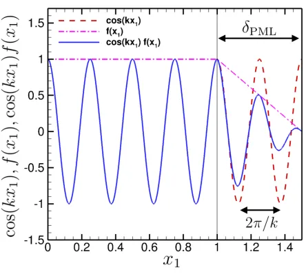
Figure 2: Plot of the real part of the 1D travelling solution, cos(kx1) (dashed line) and its counterpart after the PML coordinate transformation, Re(u) = cos(kx1)f(x1) (solid line). The thin vertical line indicates the outer boundary of the computational domain.

this purpose we note that the plot of the real part of the solution, Re(u) =

cos(kx1)f(x1), and its constituent factors in Fig. 2 shows that the number of

el-ements in the PML region required to accurately represent this solution depends

on the ratio of the PML thickness,δPML to the wavelength 2π/k, i.e. it is

con-trolled by the value of the normalised PML thickness,kδPML. IfkδPML=O(1),

the exact solution oscillates within the PML region (as in Fig. 2) and can

therefore only be resolved by a large number of finite elements. Conversely, as

kδPML→0 the solution in the PML region approaches a straight line because

cos(kx1) remains virtually constant over the width of the PML region. The

so-lution can therefore be approximated to high accuracy with even a single linear

element inside the PML region. We note that the slope of the solution is

dis-continuous at the outer edge of the computational domain,∂Dc. This does not

cause any problems if the equations are discretised with Lagrange-type finite

elements which allow for such discontinuities at element boundaries.

best if the PML thickness is chosen such thatkδPML1. However, we expect

that in actual computations there will be a lower limit of δPML beyond which

the distortion of the elements in the PML region will cause numerical problems.

Furthermore, the analysis presented so far only applies to planar waves. In

the next section we will therefore present the results of comprehensive

numer-ical experiments by which we explore these ideas for a number of increasingly

challenging test cases.

3.2. Numerical Experiments

To assess the effect of variations in the PML thicknessδPML on the quality

of actual numerical solutions we performed numerical experiments using a

stan-dard Galerkin discretisation of the transformed Helmholtz equation (6),

employ-ing Lagrange-type finite elements with linear, quadratic or cubic basis functions.

The equations were implemented inoomph-lib, the open-source object-oriented

multi-physics finite element library [29], freely available athttp://www.oomph-lib.org.

SuperLU, a sparse direct solver [30], was used to solve the linear systems.

In test cases where an exact solution, uex, is available we characterised the

accuracy of the numerical solution, uFE, in terms of the normalised L2 error,

computed over the domain of interest,Dc, (excluding the PML regions),

E =

R

Dc|uFE−uex| 2 _dx

1 dx2

R

Dc|uex| 2 _dx

1 dx2

!1/2

. (15)

The integration is always carried out on the mesh on which the actual

compu-tation is performed, using the same elemental Gauss integration scheme that

is used to evaluate the finite element matrices and vectors. In cases where an

analytical solution is known, we evaluated uex directly at the relevant Gauss

points. In cases where no exact solution is available and the reference solution

was pre-computed on a finer mesh, we evaluated the equivalent of uex on the

3.2.1. Test case 1: A one-dimensional waveguide

We start with the simple, quasi-one-dimensional test case discussed in

sec-tion 3.1 and solve the Helmholtz equasec-tion in the rectangular domain Dc =

{(x1, x2)| x1 ∈[0,1]; x2 ∈[0, H]}. The application of the Dirichlet boundary

conditionu= 1 at the left boundary (at x1 = 0), and homogeneous Neumann

boundary conditions∂u/∂n=±∂u/∂x2= 0 at the top and bottom boundaries

(at x2 = 0 and x2 = H, respectively) makes the 1D travelling wave solution

(10) the exact solution of this problem.

Since the solution is independent ofx2we discretiseDcusing a single row of

(square) quadrilateral elements of constant edge lengthhand set the (arbitrary)

height of the domain toH =h. We then aim to suppress reflections off the right

boundary (atx1= 1) with a PML region of widthδPML, which we discretise with

another NPML (rectangular) quadrilateral elements. We apply homogeneous

Neumann boundary conditions at their top and bottom boundaries, and the

homogeneous Dirichlet condition u= 0 atx1 = 1 +δPML. With this setup it

is possible to perform computations with very large numbers of elements per

wavelength since the total number of unknowns in the problem increases linearly

withN.

Fig. 3 shows the dependence of the error,E, on the normalised PML

thick-ness, kδPML, for a range of wavenumbers (k = 8,16,32 and 64) and different

numbers of elements in the PML region (NPML= 1,2,4,8 and 16, distinguished

by the different symbols). For all computations shown in this figure, we used

piecewise quadratic basis functions (p= 2), and set the number of elements per

wavelength in Dc toN = 100 to ensure that E is dominated by the error due

to the PML.

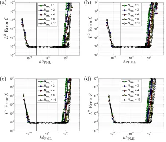
The figure shows a very robust behaviour that is consistent with the analysis

presented in section 3.1. SinceNPML is kept constant along the various curves,

an increase in δPML makes it more and more difficult to resolve the solution

in the PML region. A rise inkδPML beyond≈10−2 therefore leads to a rapid

(a)

(b)

(c)

(d)

Figure 3: ErrorEas a function of the normalised PML thickness,kδPML, and the number of element layers in the PML region,NPML, for Test Case 1. (a)k= 8, (b)k= 16, (c)k= 32, (d)

obviously incurs additional computational cost.

For smaller values of the PML thickness, the solution in the PML region

is sufficiently close to a linear function of x1 that it is easy to resolve with a

very small number of elements. As a result, in this regime the error obtained

forNPML= 1 is practically identical to that obtained with a much finer spatial

resolution (e.g. NPML = 16). This is illustrated further in Fig. 4 where we

plot the exact (solid lines) and computed (dashed lines) solutions fork= 8 for

three different values of the PML thickness. All computational results in this

figure were obtained with linear elements (p = 1) and a fine bulk

discretisa-tion (N = 100) to ensure that the error is dominated by the presence of the

PML region which we discretised with a single element, NPML = 1. The left

column shows the overall solution; in the right column we plot the solutions

near the boundary of the computational domain as a function of the normalised

coordinateν1/δPML, where ν1 =x1−1 is the distance from the outer edge of

the computational domain. This normalisation ensures that the PML region

is always located between 0 and 1 and facilitates the comparison between the

solutions for different PML thicknesses. The oscillations of the exact solution in

the PML region forδPML= 1.0 (shown in the top row of the figure) can clearly

not be resolved by this discretisation and the error in the overall solution is

therefore very large. A reduction in δPML reduces the number of waves that

are contained in the PML region and this greatly improves the accuracy of the

computed solution. For δPML = 10−6 (in the bottom row of the figure), the

exact and computed solutions become graphically indistinguishable.

Returning now to Fig. 3, we observe that for even smaller PML thicknesses,

kδPML<10−8, when the elements in the PML region become rather distorted,

the errorE increases again. We performed numerical experiments to show that

the rise in the error in this regime is correlated with the rapidly increasing

inaccuracy of the numerical integration scheme. In all our computations the

elements’ contributions to the matrix and right hand side of the global linear

system that determines the solution were computed with “full integration”,

Figure 4: The exact (solid lines) and computed (dashed lines) solutions for Test Case 1 for

basis functions exactly (this requires the use of (p+ 1)×(p+ 1)-node

tensor-product Gauss rules for quadrilateral elements with basis functions of orderp;

see, e.g., [31]). We compared the entries in the numerically computed elemental

matrices against their exact counterparts, obtained by evaluating the relevant

integrals usingmaple. As expected, the elemental matrices associated with

el-ements in the bulk (for which the integrands are low-order polynomials inx1)

were found to be accurate to machine precision, while those associated with

ele-ments in the PML region generally contained small errors because the presence

of the singular absorbing functions (9) in the transformed Helmholtz equation

(6) turned the integrands into rational functions. Interestingly, the error

intro-duced by the numerical integration only became significant in a regime when

even the evaluation of the exact integrals inmaplebecame numerically difficult

and required the computations to be performed with 200 digits, indicating that

in this regime roundoff errors are beginning to have an increasingly detrimental

effect on the accuracy of the computation.

We note that for very small values ofδPML the bulk and PML meshes

con-tain elements of extremely different sizes. This has the potential to cause

ill-conditioning of the finite element matrix which may limit the accuracy of the

solution of the linear system by the direct solver. We investigated this

possi-bility by monitoring the condition number of the finite element matrices which

we found to display only a very modest increase with a reduction in δPML.

The assumption that this increase is insignificant is confirmed by the fact that

oomph-libactually treats all problems as nonlinear and solves the discretised

equations by Newton’s method. For linear problems with well-conditioned

fi-nite element matrices this method converges in one iteration. Based on our

experience with other problems, ill-conditioning of the finite element matrix

tends to result in additional Newton iterations or even cause the convergence

of the Newton method to stall. None of this behaviour was observed in any of

the computations we performed. Ill-conditioning of the finite element matrix is

therefore unlikely to be responsible for the increase in the error at small PML

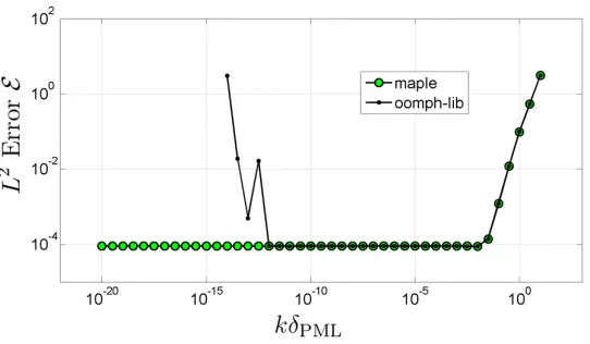
Figure 5: Error E as a function of the normalised PML thickness, for Test Case 1 with

k= 8, discretised with N = 250 linear elements per wavelength in the bulk and a single element in the PML,NPML = 1. The small markers show the error obtained when using our finite element codeoomph-lib. The larger markers represent the error obtained when the entire finite-element computation is performed inmaple, using an accuracy of 200 digits when evaluating symbolic expressions numerically.

This explanation for the rise of the error at extremely small values ofkδPML

is further supported by Fig. 5, which shows a plot of the error as a function of

the normalised PML thickness,kδPML, for the same discretisation as in Fig. 4

(linear elements, a single element in the PML region butN = 250 elements per

wavelength in the bulk). The small markers show the error when solving the

equations with our finite element code, within which the integrals are evaluated

numerically and all computations are performed in double precision arithmetic.

The larger markers show the error obtained when re-implementing the entire

finite element computation in maple, evaluating all integrals analytically and

performing the final floating point evaluation of the results with an accuracy of

200 digits. Over most of the range of PML thicknesses both formulations give

exactly the same result, but themaplecomputation does not display the rise in

the error for extremely small values ofkδPML. In fact, it is possible to

analyt-ically perform the limitkδPML→0 withinmaple. The result obtained for this

shown in this plot. While performing these computations we also monitored the

condition number of themaple-generated finite-element matrix. We found that

it also tended to a constant as kδPML was reduced. The limiting value agreed

with the condition number of the finite-element matrix obtained by actually

settingδPML= 0. This proves that the rise in the error for small values of the

PML thickness observed in Fig. 3 is due to the use of numerical integration in

the evaluation of the finite-element matrices, and the finite precision arithmetic

employed in the code. We note that, since the elements in the PML region are

right-angled quadrilaterals, the contributions to the finite-element matrix and

the right hand side of the linear system could, in principle, be computed

ana-lytically, thus bypassing the error due to the numerical integration. Appendix

A in [25] lists the relevant integrals for the case of linear elements.

The key feature that emerges from the results presented in Fig. 3 is the

existence of a large intermediate range of PML layer thicknesses,

Iopt={kδPML |10−8< kδPML<10−2}, (16)

within which the error remains approximately constant and close to its overall

minimum, virtually independent of NPML. This parameter regime is

charac-terised by the fact that within it the PML thickness is so small that the

solu-tion in the PML region is close to linear (and therefore easy to represent on a

finite element mesh) but not so small that the numerical integration of the finite

element matrices becomes difficult.

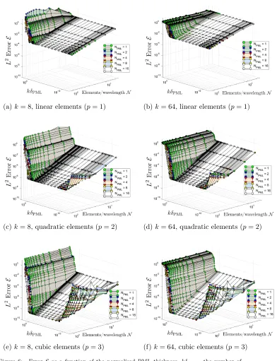
Fig. 6 shows that the features observed in Fig. 3 (forN = 100 and piecewise

quadratic basis functions) are independent of the type of basis functions, and are

not affected by variations in the bulk discretisation in the sense that for all values

ofN in the range 5≤ N ≤100, the error is small and insensitive to changes

in the normalised PML layer thickness if kδPML ∈ Iopt. In all cases the error

increases rapidly once the thickness of the PML layer exceeds kδPML >10−2.

Conversely, the increase in E for very small PML thicknesses only arises once

the bulk discretisation is sufficiently fine so that the error drops belowO(10−4_).

(a)k= 8, linear elements (p= 1) (b)k= 64, linear elements (p= 1)

(c)k= 8, quadratic elements (p= 2) (d)k= 64, quadratic elements (p= 2)

(e)k= 8, cubic elements (p= 3) (f) k= 64, cubic elements (p= 3)

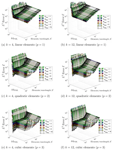
Figure 6: ErrorE as a function of the normalised PML thickness,kδPML, the number of elements per wavelength in the bulk,N, and the number of element layers in the PML region,

Berm´udezet al.’s absorbing function (9) yields optimal results for a given

com-putational cost if it is applied with a normalised PML layer thickness from the

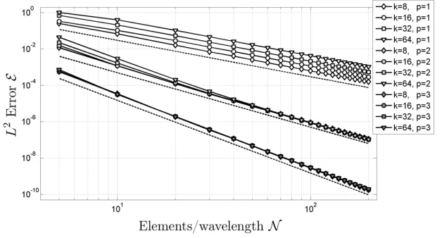
optimal range Iopt. In fact, Fig. 7 demonstrates that for the specific choice

δPML = 10−6, so that kδPML ∈Iopt (and a single element in the PML region,

NPML= 1) theL2error behaves like E ∼ N−(p+1) (forp= 1,2 and 3) asN is

increased, indicating that the error is completely controlled by the discretisation

of the bulk mesh. We refer to [32, 33, 34] for a discussion of the optimal

con-vergence rate of numerical solutions obtained from finite element discretisations

of the Helmholtz equation and note that the observed convergence rate

indi-cates that the bulk discretisation was always sufficiently fine to avoid dispersion

errors.

Figure 7: ErrorEfor Test Case 1 as a function of the number of elements per wavelength in

the bulk,N, for various wavenumbers (k= 8,16,32,64) and element types (p= 1,2,3). The PML discretisation is held fixed atδPML= 10−6 andNPML= 1. The dashed lines indicate the optimal convergence rates under bulk mesh refinementE ∼ N−(p+1)_.

3.2.2. Test case 2: Scattering of a planar wave off a cylinder

Guided by the insight obtained from the study of the simple

quasi-one-dimensional model in the previous section, we now explore the approach in a

equation (1) representing outward propagating waves is given by

u(r, θ) =

∞

X

n=−∞

An Hn(1)(kr) exp(inθ), (17)

where (r, θ) are cylindrical polar coordinates. TheAn are constant coefficients

which are determined by the boundary conditions. For the numerical

experi-ments presented below we chose

An =−

inJn(k)

Hn(1) 0

(k)

. (18)

With this choice, the solution (17) represents the scattered field generated by

a planar sound wave, propagating in thex1-direction, interacting with an

im-penetrable (sound-hard) cylinder of unit radius, centred at the origin of the

coordinate system [35]; see Fig. 1 for a contour plot of this solution, which

we obtained in a computational domain bounded by the lines x1 = ±2 and

x2=±2.

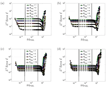
Fig. 8 shows the variation of the error withkδPML, as in Fig. 3, again for

a discretisation with piecewise quadratic basis functions,p= 2. (The range of

wavenumbers considered here is smaller because the computational cost of the

numerical simulations performed to obtain these results is significantly greater

than in the quasi-one-dimensional case; the simulations withk= 12 involved up

to 1.7 million unknowns.) We note that many features of Fig. 3 are observed

here too. Specifically, forkδPML<10−8, the error increases with a reduction in

the PML thickness. For larger values of the PML thickness the error is again

virtually independent ofkδPML, until beyondkδPML= 10−2the error begins to

vary strongly with the thickness of the PML region. Careful adjustment ofδPML

in the regime wherekδPML=O(1) (the range in which most previous attempts

at PML optimisation have been performed) allows a reduction of the error by

another order of magnitude. However, the precise value for which this optimum

is achieved depends sensitively onNPML and small changes to δPML from its

global optimum can lead to a large increase in the error. Ultimately, the error

(a) (b)

(c) (d)

Figure 8: ErrorE as a function of the normalised PML thickness,kδPML, and the number of element layers in the PML region,NPML, for Test Case 2. (a)k= 2, (b)k= 4, (c)k= 8, (d)k= 12. All computations were performed withN = 50 elements per wavelength in the bulk and quadratic basis functions,p= 2. The vertical lines delimit the optimal parameter regimeIoptwithin which the error is small and insensitive to changes in the thickness of the PML region.

PML region becomes insufficient to resolve the spatial variations of the solution

in this region.

An important difference to the results shown in Fig. 3 is that if kδPML

is chosen from the optimal range the error displays a marked dependence on

the number of element layers in the PML region, with an increase in NPML

consistently reducing the error (at additional computational cost). To explain

this observation, Fig. 9 shows how the error depends on the bulk discretisation

(a)k= 4, linear elements (p= 1) (b)k= 12, linear elements (p= 1)

(c)k= 4, quadratic elements (p= 2) (d)k= 12, quadratic elements (p= 2)

(e)k= 4, cubic elements (p= 3) (f) k= 12, cubic elements (p= 3)

Figure 9: ErrorE as a function of the normalised PML thickness,kδPML, the number of elements per wavelength in the bulk,N, and the number of element layers in the PML region,

vary between 2 and 50). Overall, the figure is very similar to its counterpart for

the quasi-one-dimensional case (Fig. 6). For a given discretisation of the PML

region (i.e. for fixedNPML andkδPML∈Iopt) an increase in the bulk resolution

(via an increase inN) initially reduces the error at the optimal rateE ∼ N−(p+1)

(see also Fig. 10), with little dependence onNPMLandkδPML, exactly as in Fig.

6). However, once the bulk discretisation has become sufficiently fine, the overall

error saturates and becomes dominated by the error due to the discretisation

of the PML region. The onset of the saturation can be delayed (and hence the

reduction in the error with an increase in N continued to larger values of N)

by increasingNPML (at additional computational cost).

The saturation of the error under bulk mesh refinement is illustrated more

clearly by the plots in Fig. 10, which show the variation of the error with an

increase inN forδPML= 10−6, such thatkδPML∈Iopt, for various wavenumbers

(k= 4,8,12), basis functions (p= 1,2,3) and values ofNPML. We note that the

dependence of the error displayed in Fig. 10 onN and NPML is well described

by a relation of the form

E(N, NPML) =CN−(p+1)+EPML(NPML) (19)

whereC is a constant that depends only weakly onk, andEPML(NPML) defines

the minimum error achievable with a given number of element layers in the

PML region. EPML(NPML) decreases approximately linearly with an increase in

NPML. It is interesting to note that the saturation of the error under increasing

bulk mesh refinement is not present in the corresponding results for Test Case

1, confirming, yet again, that Berm´udezet al.’s attenuation function is perfect

(so that there is zero reflection from the PML layer into the bulk, at least in

the continuous setting) only for planar waves.

3.2.3. Test case 3: Scattering off multiple polygonal scatterers

Finally, we assess the performance of our approach in a multiple-scattering

problem in which an incoming planar wave, travelling in the negativex1-direction,

Linear elements (p= 1)

(a)k= 4 (b)k= 8 (c)k= 12

Quadratic elements (p= 2)

(d)k= 4 (e) k= 8 (f)k= 12

Cubic elements (p= 3)

(g)k= 4 (h)k= 8 (i)k= 12

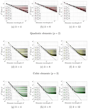
Figure 10: ErrorE for Test Case 2 as a function of the number of elements per wavelength

in the bulk,N, for various wavenumbers (k= 4,8,12) and element types (p= 1,2,3). The PML discretisation is held fixed atδPML = 10−6. The dashed lines indicate the optimal convergence rates under bulk mesh refinement,E ∼ N−(p+1)_{. The white symbols indicate}

the point at which the error is deemed to start saturating, based on the criteria used in section

which we apply the Neumann boundary condition

∂u

∂n = ikn1exp(−ikx1), (20)

wheren= (n1, n2) is the outer unit normal on∂DN. Fig. 11 shows the real part

of the scattered field fork= 40, computed on a very coarse mesh with a thick

PML region. A key feature of this problem is that the sharp re-entrant corners

on the surface of the scatterer create a derivative singularity in the solution

which limits the asymptotic convergence rate of the numerical solution under

mesh refinement. Since there is no exact solution for this problem, we use the

numerical solution computed withN = 180, a PML layer thickness ofδPML =

10−6 _{and N}

PML = 16 as a proxy for uex. This involved the most expensive

simulations performed in this study and required in excess of 10 million degrees

of freedom for the most refined simulations with cubic elements.

6

-x

x

-1

Figure 11: Plot of the solution of Test Case 3 for a wavenumber ofk= 40 computed on a very coarse finite element mesh surrounded by a (relatively thick) PML.

by the vertical lines in Fig. 12(a) again leads to a minimal error for fixed values

of the discretisation parametersN and NPML (here kept fixed at N = 22 and

NPML= 16) for linear, quadratic and cubic basis functions. Furthermore, Fig.

12(b) shows that for the specific choiceδPML= 10−6, such that kδPML∈Iopt,

the error decays at the same rate E ∼ N−5/3 _{(shown by the dashed line) for}

all types of basis functions. This is consistent with the theoretically expected

behaviour for domains with sharp re-entrant corners; see e.g. [36] for a discussion

in the context of the Poisson equation.

We note that unlike the behaviour shown in Fig. 10, the error in Fig. 12(b)

does not display any saturation under bulk mesh refinement, despite the fact

that the scattered waves impinging on the PML boundary are non-planar. This

is due to the fact that the error displayed in Fig. 12(b) was computed by

referring to a numerical solution that was computed on a finer bulk mesh (larger

N) but with the same number of element layers in the PML region (sameNPML).

Assuming that the actual error (relative to the (unknown) exact solution) in

both numerical solutions has the functional form (19), the saturation errorEPML

is expected to cancel out. The absence of the saturation in Fig. 12(b) therefore

provides further support for our conjecture that the actual error associated with

Berm´udezet al.’s PML depends on the discretisation parametersN, NPMLand

pas described by equation (19). We have performed additional computations to

confirm that the saturation error re-appears if the reference solution is computed

with a larger number of elements in the PML region.

3.3. The saturation of the error for non-planar waves

The numerical results presented so far indicate that for a fixed computational

effort (i.e. constant p, N and NPML) there exists a range of normalised PML

thicknesses such that for kδPML ∈ Iopt, the error remains small and typically

close to the global minimum achievable. If the thickness of the PML region is

chosen from within this range, the error may be reduced further by p-refinement,

i.e. an increase in the order of the elements’ basis functions; the benefit of

(a) (b)

Figure 12: Results for Test Case 3 withk= 40. (a) ErrorEas a function of the normalised PML thickness,kδPMLforN = 22 andNPML = 16. The vertical lines delimit the optimal parameter regimeIopt defined in equation (16). (b) ErrorEas a function of the number of elements per wavelength in the bulk, N, for three elements types (p = 1,2,3). The PML discretisation is held fixed atδPML= 10−6 andNPML= 16. The dashed line indicates the optimal convergence rate under bulk mesh refinement,E ∼ N−5/3_.

to saturate with increasingN (unless the solution consists of planar waves for

which Berm´udezet al.’s [25] PMLs cause practically no reflection).

Since the onset of the saturation can be delayed by an increase in NPML

(see also [21, 23]), it is desirable to determine the minimum number of element

layers in the PML region,N_PMLmin, that is required to ensure that the quality of

the numerical solution is controlled exclusively by the bulk discretisation so that

for sufficiently smooth solutions the dependence of the error on the parameters

N andpfollows the asymptotic behaviourE ∼ N−(p+1)_{. To determine the}

de-pendence ofNmin

PMLonN based on this criterion we note that in the log-log plots

in Fig. 10 the curves representing the error for fixedNPMLcontain two

approx-imately straight segments – one in the region where the error decays according

to the asymptotic error estimate, the other where the error has saturated and

remains constant. To determine the transition between these two regimes (and

thus the onset of the saturation) we fitted a spline to each of these curves and

particular value ofNPMLfirst deviated from the theoretical convergence rate by

more than 10%. The pairs (Nb, NPML) obtained by this procedure are shown by

the white symbols in Fig. 10. They define the valueNPML required to

(approx-imately) retain the theoretical convergence rate under bulk mesh refinement up

to the spatial resolution associated withNb and thus defineN_PMLmin (N).

Fig. 13 indicates howNmin

PML varies withN for the data from Test Case 2.

The range over which data is displayed in Fig. 13 is determined by the range

ofN over which saturation is observed in Fig. 10. For linear elements (p= 1),

b

N approaches the maximum value of N considered (N ≤ 120), while for the

higher-order elements (p= 2,3) saturation is observed at more modest values

ofN so that the original data is limited by the maximum number of element

layers in the PML region (NPML ≤ 40). Additional computations with up to

NPML = 240 were therefore performed to extend the range of data available.

Fig. 13 shows that in all cases the number of element layers in the PML region

must increase linearly with the number of elements per wavelength in the bulk

to retain the asymptotic convergence rate under (bulk) mesh refinement. While

higher-order elements require much larger numbers of elements in the PML

region to achieve this, it is important to stress that they tend to be much more

accurate than their low-order counterparts and always give far more accurate

results for given values ofN andNPML.

4. Summary and Conclusions

We have provided an alternative interpretation of Berm´udez et al.’s

obser-vation that, in a continuous setting, PMLs that are based on the unbounded

damping function (9) do not cause any reflections for planar waves. This

al-lowed us to show that, when discretised with conforming Lagrange-type finite

elements, such PMLs perform best (for a given computational effort) when their

thickness is chosen such thatkδP M L 1, i.e. if the thickness of the PML

re-gion is much smaller than the wavelength. Motivated by this observation we

nor-(a) k=4 (b) k=8 (c) k=12

Figure 13: The minimum number of element layers in the PML region,Nmin

PML, required to

maintain the optimal convergence rate under bulk mesh refinement for a)k= 4, b)k= 8 and c)k= 12 and the three element types (p= 1,2 and 3) considered in this study. The thick solid lines are straight lines through the data points for largeN. PML thicknessδPML= 10−6 for all cases.

malised PML thicknesses, Iopt, such that for kδPML ∈ Iopt Berm´udez et al.’s

unbounded absorbing function (9) yields an error that is optimal (in the sense

of being both small and insensitive to change) for a given computational cost

(number of elements in the bulk and in the PML regions). Within the optimal

parameter regime, the error remains small and virtually constant over several

orders of magnitude of the normalised PML thickness kδPML. The optimal

regime is bounded above by a regime in which the error increases due to

insuffi-cient spatial resolution in the PML region, and below by a regime in which the

numerical integration becomes inaccurate. We stress that the optimal choice of

the PML thickness does not require further optimisation within Iopt since the

error is virtually constant within this range. As long as kδPML is chosen from

withinIoptits actual value is irrelevant since it neither affects the error nor the

computational cost. Our recommendation to choose the normalised PML

thick-nesskδPMLfrom anywhere within the optimal regimeIopttherefore makes PML

optimisation unnecessary and thus makes Berm´udez et al.’s PMLs parameter

free.

lay-ers in the PML region, NPML, the error is controlled exclusively by the bulk

discretisation, which we characterised in terms of the number of elements per

wavelength,N. For a PML thickness from the optimal range, the error follows

the theoretical error estimate (E ∼ N−(p+1)_{for smooth solutions andE ∼ N}−5/3

for solutions with derivative singularities) until the presence of the PML causes

a saturation of the error under further bulk mesh refinement. The saturation in

the error can be delayed by an increase inNPML (at additional computational

cost). We showed that a linear increase inNPMLtogether with an increase inN

suffices to retain the theoretical convergence rate under bulk mesh refinement;

see also [21, 23].

We note that Berm´udezet al. introduce a whole family of unbounded

damp-ing functions (types A-D, which all have a free parameter, β). They all share

the property that, in the continuous setting, they completely suppress the

re-flection of planar waves with arbitrary incidence angle. In recent years other

authors (e.g. [37, 38]) have also considered this class of functions and have

conducted studies on the variation of the various parameters in their respective

formulations (e.g. [26, 39]). It is therefore important to stress that the damping

function (9) used in the present paper isthe onlyfunction that has the key

prop-erty that the complex coordinate mapping (11) transforms a planar travelling

wave (10) into a linear function within the PML region as kδPML → 0. It is

interesting to note that Berm´udez et al. determined the optimal value of their

parameterβ via numerical experiments. These suggested β= 1 – precisely the

value required to turn their type A function into (9). We refer to the Appendix

for a more detailed discussion of Berm´udezet al.’s other unbounded damping

functions.

As in Berm´udez et al.’s paper, our theoretical analysis applies only to the

case of planar waves. We employed extensive numerical experiments to explore

the optimal PML thickness in other settings. Given that these experiments

in-cluded test cases with a variety of solution types (planar and non-planar waves;

domains with smooth and polygonal boundaries; smooth and singular solutions;

differ-ent elemdiffer-ent types and an extremely wide range of spatial resolutions, we have

confidence in the general nature of our results. Following the suggestion of a

ref-eree, we also explored the behaviour of Berm´udezet al.’s damping function with

spectral elements (using nodal Legendre bases of various orders). The

simula-tions (not presented here) showed the same behaviour that we reported for the

low-order Lagrange-type finite elements. We suspect that our recommendation

for the optimal thickness of the PML region also applies to the 3D Helmholtz

equation, though the computational cost of performing equally comprehensive

numerical experiments on 3D test problems would be considerable. It will be

interesting to explore the performance of Berm´udez et al.’s absorbing functions

in other wave equations, such as the equations of time-harmonic linear elasticity,

to assess if our recommendation for the optimal thickness of the PML region

applies here too. This work is currently in progress.

Acknowledgements

We would like to acknowledge the financial support of Thales UK Limited

and the School of Mathematics at the University of Manchester. We are

grate-ful to Phil Cotterill and Robert Harter for their comments on a draft of this

manuscript. We also wish to thank the referees for their constructive comments

and suggestions.

References

[1] A. Sommerfeld, Partial Differential Equations in Physics, Academic Press,

New York, 1949.

[2] B. Engquist, A. Majda, Absorbing boundary conditions for the numerical

simulation of waves, Mathematics of Computation 31 (139) (1977) 629–651.

[3] R. Mittra, O. Ramahi, Absorbing boundary conditions for the direct

problems. PIER 2: Finite Element and Finite Difference Methods in

Elec-tromagnetic Scattering., M.A. Morgan, Elsevier, New York, 1990.

[4] A. Bayliss, M. Gunzburger, E. Turkel, Boundary conditions for the

nu-merical solution of elliptic equations in exterior regions, SIAM Journal on

Applied Mathematics 42 (1982) 430–451.

[5] J. Jin, The Finite Element Method in Electromagnetics, 2nd Edition,

Wiley-Blackwell, New York, 2002.

[6] D. Givoli, High-order local non-reflecting boundary conditions: a review,

Wave Motion 39 (2003) 319–326. doi:10.1016/j.wavemoti.2003.12.004.

[7] S.-K. Jeng, C.-H. Chen, On variational electromagnetics: theory and

ap-plication, IEEE Transactions on Antennas and Propagation 32.

[8] R.-B. Wu, C. Chen, Variational reaction formulation of scattering problem

for anisotropic dielectric cylinders, IEEE Transactions on Antennas and

Propagation 34 (5) (1986) 640–645. doi:10.1109/TAP.1986.1143874.

[9] L. Pearson, R. Whitaker, L. Bahrmasel, An exact radiation boundary

con-dition for the finite-element solution of electromagnetic scattering on an

open domain, IEEE Transactions on Magnetics 25 (4) (1989) 3046–3048.

doi:10.1109/20.34364.

[10] K. Ihlenburg, Finite Element Analysis of Acoustic Scattering,

Springer-Verlag, New York, 1998.

[11] J.-P. B´erenger, A perfectly matched layer for the absorption of

electromag-netic waves, Journal of Computational Physics 114 (2) (1994) 185 – 200.

doi:http://dx.doi.org/10.1006/jcph.1994.1159.

[12] I. Harari, A survey of finite element methods for time-harmonic

acous-tics, Computer Methods in Applied Mechanics and Engineering 195 (1316)

(2006) 1594 – 1607, a Tribute to Thomas J.R. Hughes on the Occasion of

[13] X. Yuan, D. Borup, J. Wiskin, M. Berggren, R. Eidens, S. Johnson,

Formulation and validation of Berenger’s PML absorbing boundary for

the FDTD simulation of acoustic scattering, IEEE Transactions on

Ul-trasonics, Ferroelectrics, and Frequency Control 44 (4) (1997) 816–822.

doi:10.1109/58.655197.

[14] D. Komatitsch, R. Martin, An unsplit convolutional perfectly matched layer

improved at grazing incidence for the seismic wave equation, Geophysics

72 (5) (2007) SM155–SM167. doi:10.1190/1.2939484.

[15] D. Komatitsch, J. Tromp, A perfectly matched layer absorbing boundary

condition for the second-order seismic wave equation, Geophysical Journal

International 154 (1) (2003) 146–153.

[16] U. Basu, A. Chopra, Perfectly matched layers for time-harmonic

elasto-dynamics of unbounded domains: theory and finite-element

implementa-tion, Computer Methods in Applied Mechanics and Engineering 192 (2003)

1337–1375. doi:10.1016/S0045-7825(02)00642-4.

[17] G. Cohen, S. Fauqueux, Mixed spectral finite elements for the linear

elastic-ity system in unbounded domains, SIAM Journal on Scientific Computing

26 (3) (2006) 864–884. doi:10.1137/S1064827502407457.

[18] K. Meza-Fajardo, A. Papageorgiou, A nonconvolutional, split-field,

per-fectly matched layer for wave propagation in isotropic and anisotropic

elas-tic media: Stability analysis, Bulletin of the Seismological Society of

Amer-ica 98 (4) (2008) 1811–1836. doi:10.1785/0120070223.

[19] Y. Ukai, S. Ishida, N. Hata, T. Azuma, S. Umemura, T. Dohi, A 3−d

simulation of focused ultrasound propagation for extracorporeal shock wave

osteotomy, International Congress Series 1256 (1) (2003-06-01T00:00:00)

658–663. doi:10.1016/S0531-5131(03)00278-4.

ab-sorbers for finite-element mesh truncation, IEEE Transactions on Antennas

and Propagation 45 (3) (1997) 474–486. doi:10.1109/8.558662.

[21] G. Pan, A. Abubakar, T. Habashy, An effective perfectly matched

layer design for acoustic fourth-order frequency-domain finite-difference

scheme, Geophysical Journal International 188 (1) (2012) 211–222.

doi:10.1111/j.1365-246X.2011.05244.x.

[22] E. B´ecache, A.-S. B.-B. Dhia, G. Legendre, Perfectly matched layers for

the convected Helmholtz equation, in: G. C. Cohen, P. Joly, E. Heikkola,

P. Neittaanmki (Eds.), Mathematical and Numerical Aspects of Wave

Propagation WAVES 2003, Springer Berlin Heidelberg, 2003, pp. 142–147.

doi:10.1007/978-3-642-55856-6-23.

[23] I. Singer, E. Turkel, A perfectly matched layer for the Helmholtz equation

in a semi-infinite strip, Journal of Computational Physics 201 (2) (2004)

439–465. doi:10.1016/j.jcp.2004.06.010.

[24] X. Jiang, W. Zheng, Adaptive perfectly matched layer method

for multiple scattering problems, Computer Methods in

Ap-plied Mechanics and Engineering 201204 (0) (2012) 42 – 52.

doi:http://dx.doi.org/10.1016/j.cma.2011.09.013.

[25] A. Berm´udez, L. Hervella-Nieto, A. Prieto, R. Rodr´ıguez, An optimal

per-fectly matched layer with unbounded absorbing function for time-harmonic

acoustic scattering problems, Journal of Computational Physics 223 (2)

(2007) 469 – 488. doi:http://dx.doi.org/10.1016/j.jcp.2006.09.018.

[26] D. Rabinovich, D. Givoli, E. B´ecache, Comparison of high-order absorbing

boundary conditions and perfectly matched layers in the frequency domain,

International Journal for Numerical Methods in Biomedical Engineering

26 (10) (2010) 1351–1369. doi:10.1002/cnm.1394.

[27] F. Teixeira, W. Chew, A general approach to extend Berenger’s

Transactions on Antennas and Propagation 46 (9) (1998) 1386–1387.

doi:10.1109/8.719984.

[28] S. Kucukcoban, L. Kallivokas, A symmetric hybrid

formu-lation for transient wave simulations in PML-truncated

het-erogeneous media, Wave Motion 50 (1) (2013) 57 – 79.

doi:http://dx.doi.org/10.1016/j.wavemoti.2012.06.004.

[29] M. Heil, A. L. Hazel,oomph-lib– an object-oriented multi-physics

finite-element library, in: M. Sch¨afer, H.-J. Bungartz (Eds.), Fluid-Structure

Interaction, Springer, 2006, pp. 19–49, oomph-lib is available as

open-source software athttp://www.oomph-lib.org.

[30] J. W. Demmel, S. C. Eisenstat, J. R. Gilbert, X. S. Li, J. W. H. Liu, A

supernodal approach to sparse partial pivoting, SIAM Journal on Matrix

Analysis and Applications 20 (3) (1999) 720–755.

[31] K.-J. Bathe, Finite element procedures, 2nd Edition, Prentice-Hall,

Engle-wood Cliffs, 1996.

[32] F. Ihlenburg, I. Babu˘ska, Solution of Helmholtz problems by

knowledge-based FEM, Computer Assisted Mechanics and Engineering Sciences 4

(1997) 397–415.

[33] I. Babu˘ska, M. Suri, The p and h-p versions of the finite element method,

basic principles and properties, SIAM Review 36 (1994) 4:578–632.

[34] I. Babu˘ska, F. Ihlenburg, E. Paik, S. Sauter, A generalized finite element

method for solving the Helmholtz equation in two dimensions with minimal

pollution, Computer Methods in Applied Mechanics and Engineering 128

(1995) 325–359. doi:10.1016/0045-7825(95)00890-X.

[35] C. Linton, P. McIver, Handbook of mathematical techniques for

[36] H. Elman, D. Silvester, A. Wathen, Finite Elements and Fast Iterative

Solvers, Oxford University Press, Oxford, 2005.

[37] J. Kormann, P. Cobo, A. Prieto, Perfectly matched layers for

mod-elling seismic oceanography experiments, Journal of Sound and Vibration

317 (12) (2008) 354 – 365. doi:10.1016/j.jsv.2008.03.024.

[38] S. Ham, K.-J. Bathe, A finite element method enriched for wave

prop-agation problems, Computers and Structures 9495 (0) (2012) 1 – 12.

doi:10.1016/j.compstruc.2012.01.001.

[39] A. Modave, E. Delhez, C. Geuzaine, Optimizing perfectly matched

lay-ers in discrete contexts, International Journal for Numerical Methods in

Engineering 99 (6) (2014) 410–437. doi:10.1002/nme.4690.

Appendix: The performance/behaviour of other unbounded damping

functions

One of the key observations of our paper is that the damping function (9) is

the onlyfunction that has the key property that the complex coordinate mapping

(11) transforms a planar travelling wave (10) into a linear function within the

PML region askδPML→0. This observation explains why for sufficiently small

values of the PML thickness even a single linear element suffices to represent

the exact solution of the coordinate-transformed Helmholtz equation (6) within

the PML region, implying that the accuracy of the overall solution is controlled

exclusively by the bulk discretisation.

Berm´udezet al. [25] introduce a much wider class of unbounded damping

functions which all have the property that, in the continuous setting, they yield

zero reflection from the boundary of the computational domain. Our

analy-sis suggests that their performance in a finite-element-based discretisation will

depend crucially on how easy it is resolve this exact solution within the PML

(which we discuss below), Berm´udez et al. [25] consider four different

damp-ing functions, Types A-D. All of these transform the travelldamp-ing wave solution

u(x1) = exp(ikx1) intof(x1) exp(ikx1), where f = 1 at the interface between

the computational domain and the PML region, andf = 0 at the outer

bound-ary of the PML region where we impose (consistent) homogeneous Dirichlet

boundary conditions. The ease with which this exact solution can be

repre-sented on a finite-element mesh depends on the shape off(x1) within the PML

region.

(a) (b)

(c) (d)

Figure 14: Prefactorfas a function of the normalised coordinateν1/δPML, whereν1=x1−1 is the distance from the outer edge of the computational domain for (a) Type A, (b) Type

B, (c) Type C and (d) Type D damping profiles. We present results for PML thicknesses

δPML = 100 (dotted black lines) andδPML = 10−6 (thick coloured lines). The inset in (b) and (d) shows a zoom into the region near the interface between the computational domain

Type A:

σ(x1) =

1 1 +δPML−x1

.

This corresponds to our choice (9) and yields

f(x1) =

1 +δPML−x1

δPML

,

a straight line across the PML, irrespective of the PML thickness. See

Fig. 14(a).

Type B:

σ(x1) =

1

(1 +δPML−x1)2

This is obtained by raising the “Type A” function to the second power and

thus leads to a more rapid attenuation of the solution within the PML. It

yields

f(x1) = exp

₁

δPML

− 1

1 +δPML−x1

.

Fig. 14(b) shows that this function is highly nonlinear and becomes

in-creasingly steep near the interface between the computational domain and

the PML region as kδPML →0, making it difficult to resolve on a finite

element mesh. This function can therefore only be used for relatively large

PML thicknesses, while using a sufficient number of elements in the PML

to resolve the spatial variation to the required accuracy. The

determi-nation of the optimal values for NPML and δPML requires a case-by-case

numerical PML optimisation.

Type C:

σ(x1) =

1 1 +δPML−x1

− 1 δPML

.

This is obtained by the addition of the constant 1/δPML to the Type A

function which makes σ(x1) continuous across the interface between the

computational domain and the PML region. This may be advantageous

in certain problems because it avoids the discontinuity in the slope of the

the desirable linear variation off(x1) within the PML region by an

expo-nential,

f(x1) =

1 +δPML−x1

δPML

exp

_x

1−1

δPML

(see Fig. 14(c)), making it impossible to resolve the exact solution in

the PML with a single linear element. The shape of the scaling factor is

independent of δPML, therefore an increase in the number of elements in

the PML region, NPML (or an increase in the order of the finite element

basis function, p) suffices to reduce the error, irrespective of the PML

thickness.

Type D:

σ(x1) =

1

(1 +δPML−x1)2

− 1 δ2

PML

,

is the continuous version of the Type B function. It corresponds to

f(x1) = exp

₁

δPML

− 1

1 +δPML−x1

+x−1 δ2

PML

which suffers from the same problem as its discontinuous counterpart; see

Fig. 14(d).

(a)N = 20, NPML= 1 (b)N = 100, NPML= 1 (c)N = 100, NPML= 8

Figure 15: ErrorEfor Test Case 1 withk= 8 as a function of the normalised PML thickness,

kδPML for damping profiles of Type A-D. (a) N = 20 (b) N = 100 linear elements per wavelength in the bulk, and a single element in the PML, NPML = 1. (c)N = 100 and

Fig. 15 shows the dependence of the error on the normalised PML thickness

for the quasi-one-dimensional Test Case 1 considered in section 3.2.1. The

domain is discretised with (a)N = 20 and (b,c) N = 100 linear finite elements

per wavelength in the bulk. In (a,b) the PML contains a single linear element,

NPML= 1, while the results in (c) were obtained withNPML= 8. As expected,

the Type B and D damping functions perform very poorly for thin PMLs. The

error for the Type C function is much larger than that for the Type A function

but for kδPML ∈ Iopt the error remains approximately constant as δPML is

reduced because the variation off(x1) through the PML is independent of its

thickness. The comparison between Figs. 15(a) and (b) shows that an increase

in the bulk resolution (from N = 20 to 100 elements per wavelength) only

reduces the error for the Type A function. This is consistent with our assertion

that the error associated with the Type C solution is controlled by the overly

coarse discretisation of the PML – a single linear element cannot resolve a

function that has the same shape as that shown in Fig. 14(c). Finally, Figs.

15(b) and (c) show the effect of an increase fromNPML= 1 to 8 at a fixed bulk

resolution (N = 100). As expected, we find that for kδPML∈Iopt the Type C

solution benefits from this increase since it allows an improved resolution of the

solution in the PML. Conversely, the error associated with the Type A solution

remains unaffected since a single linear element is already sufficient to represent

the profile shown in Fig. 14(a).

Having confirmed that, of the various damping functions considered by

Berm´udez et al., the Type A function performs best, we finally consider the

effect of including a multiplicative constantB into the mapping function,

σ(x1) =

B 1 +δPML−x1

.

This yields the scaling factor

f(x1) =

_{1 +δ}

PML−x1

δPML

B .

The spatial variation of this function across the PML is independent of δPML

for all other values the linear profile is distorted and thus unnecessarily difficult

to resolve on a finite element mesh (with values in the range B < 1 being

particularly problematic because of the infinite slope off(x1) at the outer edge

of the PML). We note that the constant B is the non-dimensional equivalent

of Berm´udezet al.’s factorβ which they determined by numerical experiments

to yield optimal results if set to the wavespeedc– this corresponds precisely to