Influence of the thermo-physical properties of pavement materials on the evolution of 1
temperature depth profiles in different climatic regions 2
3
Matthew R Hall1*, Pejman Keikhaei Dehdezi1, 2, Andrew R Dawson2, James Grenfell2, Riccardo 4
Isola2 5
6
1 Nottingham Centre for Geomechanics, Division of Materials, Mechanics and Structures, Faculty of
7
Engineering, University of Nottingham, University Park, NG7 2RD, UK Tel: +44 (0) 115 846 7873, 8
Fax: +44 (0) 115 951 3159, E-mail: [email protected] 9
2 Nottingham Transport Engineering Centre, Division of Infrastructure and Geomatics, Faculty of
10
Engineering, University of Nottingham, University Park, NG7 2RD, UK 11
* Correspondence author 12
13
Abstract 14
The paper summarizes the relative influence of different pavement thermo-physical properties on the 15
thermal response of pavement cross-sections, and how their relative behaviour changes in different 16
climatic regions. A simplified one-dimensional heat flow modelling tool was developed to achieve this 17
using a finite difference solution method for studying the dynamic temperature profile within 18
pavement constructions. This approach allows for a wide variety and daily varying climatic 19
conditions to be applied, where limited or historic thermo-physical material properties are available, 20
and permits the thermal behaviour of the pavement layers to be accurately modelled and modified. 21
The model was used with available thermal pavement materials properties and with properties 22
determined specifically for the study reported here. The pavement materials included in the study 23
comprised both conventional bituminous and cementicious mixes as well as unconventional mixtures 24
that allowed a wide range of densities, thermal conductivities, specific heat capacities and thermal 25
diffusivities to be investigated. Initially, the model was validated against in-situ pavement data 26
collected in the USA in five widely differing climatic regions. It was found to give results at least as 27
good as others available from more computationally expensive approaches such as 2D and 3D FE 28
Manuscript
Click here to download Manuscript: Hall et al 2010 - temp profile pavement material- R2 version.doc
commercial packages. Then the model was used to compute the response for the same locations had 29
the thermal properties been changed by using some of the unconventional pavement materials been 30
used. This revealed that reduction of temperature range by several degrees was easily possible (with 31
implications for reduction of rutting, fatigue and the Urban Heat Island effect) and that depth of 32
penetration of peak temperatures was also achievable (with implications for winter freeze-thaw). 33
However, the results showed that there was little opportunity to displace the peak temperatures in 34
time. 35
36
Subject headings: Pavements; Heat transfer; Thermal diffusion; Temperature distribution; Numerical 37 models 38 39 Nomenclature 40
a absorptivity (-)
41
cp constant pressure specific heat capacity (J/kg K) 42
d thickness of pavement/ground element (m) 43
hc total (or mean) convection heat transfer coefficient (W/m
2
K) 44
hrad total (or mean) radiation heat transfer coefficient, = 45
i counter for time step (i = 0 corresponding to specified initial condition) 46
qabsorbed heat flux from surface absorbed solar radiation (W/m
2
) 47
qsolar heat flux fromincident solar radiation (W/m
2
) 48
Lc characteristic length, i.e. area/perimeter (m) 49
m number of nodal points (1, 2,… n) 50
Nu Nusselt number for free and forced convection (-) 51
Tsky sky temperature (K) 52
Tair ambient air temperature (K) 53
Tdp dew-point temperature (˚C) 54
T0 absolute temperature of the surface (K) 55
Tsurr surrounding temperature (K) 57
vw wind velocity (m/s) 58
α thermal diffusivity (m2/s) 59
σ Stefan-Boltzmann constant = 5.668 × 10⁻⁸ (W/m2 K4) 60
ε emissivity (-)
61
dry state thermal conductivity (W/m K) 62
d dry density (kg/m
3 ) 63 64 1. Introduction 65
Approximately half of the world‟s incoming solar energy is absorbed by the earth‟s surface 66
(RETScreen 2005), and pavements comprise large areas of our infrastructure including roads, 67
pedestrian pathways and parking areas. Temperature changes in pavements have been studied for 68
many years since they have a significant impact on pavement performance under load-induced and 69
thermal stresses and on service life. In flexible pavements (i.e. asphalt) the structural or load-carrying 70
capacity of pavement varies with temperature since hot-mix asphalt (HMA) is a visco-elastic material 71
(Ramadhan and Wahhab 1997; Marshall et al. 2001, Diefenderfer et al. 2002). In rigid pavements (i.e. 72
concrete) temperature gradients across the concrete slab can cause structural defects such as warping 73
and curling (Choubane and Tia 1992, Daiutolo 2003, Delatte 2008). Temperature variations in 74
pavements can induce freeze-thaw cycles in the pavement which can often reduce their long-term 75
stability (Dempsey & Thompson 1970). In addition, the significant contribution that pavements can 76
make to the Urban Heat Island (UHI) is well known, and previous studies have attempted to predict 77
this by numerically modelling near-surface temperature formation (Rosenfeld et al. 1998, Bretz et al. 78
1998). 79
80
In the UK, the temperature experienced in road pavements can vary between -8 °C and 60 °C, 81
depending upon location and climate, and is usually above the ambient air temperature during the 82
daytime and evening (Asaeda & Wake 1996). The US Strategic Highway Research Program (SHRP) 83
more than ten years it involved thousands of test sections at hundreds of locations throughout the USA 85
with complementary sections being built and monitored in other countries. Part of the study was the 86
Seasonal Monitoring Program (SMP) with sixty four different test locations covering a highly diverse 87
range of climatic conditions (Mohseni & Symons 1998). SMP data has since been used as a basis for 88
validation of many pavement temperature prediction models (Dempsey & Thompson 1970, Rosenfeld 89
et al. 1998, Solaimanian & Kennedy 1993, Hermansson 2000, Hermansson 2004). A significant 90
problem is to understand how material selection and pavement design affect the temperature depth 91
profile evolution, peak surface temperature, and responsiveness to climatic variables (e.g. solar 92
irradiation, air temperature, surface wind velocity). Better understanding would allow intelligent 93
design and material specification that could be tailored to match local climatic conditions. This could 94
lead to improved performance and longevity of pavements, and enable better use of the heat as a low-95
grade energy source with existing technology, e.g. surface hot water collection. Enhanced shallow heat 96
storage could be used in conjunction with ground source heat pump technology and road de-icing (van 97
Bijsterveld & de Bondt 2002, de Bondt 2003, Carder 2007). 98
99
The objectives of this study are to use a predictive transient model to determine the behavioural 100
sensitivity to pavement thermo-physical properties of 101
i) pavement surface temperature gain/loss 102
ii) temperature depth profile formation 103
iii) internal pavement temperature responsiveness in five contrasting climatic regions of the 104
USA 105
106
The practical application of this research will be to provide generalised conclusions to help inform 107
intelligent material selection and pavement design. 108
109
2. Thermo-physical properties of pavement materials 110
2.1 Past work 111
In unbound granular material (i.e. aggregates with some pore water), published data shows typical 112
thermal conductivity figures of λwater = 0.56 W/m K, λair = 0.026 W/m K and λmineral ≈ 3 W/m K,
113
varying somewhat with aggregate mineralogy (Yun & Santamarina 2008). Inter-particle contact and 114
the degree of saturation play a critical role in heat transport phenomena in such materials. For the 115
volume-averaged thermal conductivity of a representative sample of this material, the ordered 116
sequence of magnitude is: λair < λdry soil < λwater < λsat soil < λmineral (Yun & Santamarina 2008). With
117
reference to Figure 1, binder coatings increase the surface area at points of inter-particle contact, 118
theoretically increasing heat flux within the material over that of the dry loose aggregates. However, 119
the thermal conductivity of bitumen (as a binder) is relatively low, at λbitumen = 0.15 - 0.17 W/m K
120
(Hunter 2003), effectively acting as an insulative coating to aggregate particles. In contrast, hardened 121
cement paste (HCP), which is found in concrete paving materials, has a thermal conductivity of 122
approximately 0.8 – 0.9 W/m K (CES Edupack 2007). The thermo-physical properties of pavement 123
materials can be selectively modified through the use of alternative aggregates, modified binders 124
and/or void-filling conductive grouts. Further research is still needed to allow this to be done 125
intelligently and in an accurately predictable manner. A review of existing published data for thermo-126
physical properties of standard pavement and sub-soil materials has been summarised in Table 1 for 127
direct comparison with the new data presented in this study. 128
129
2.2 Present work 130
Independent experimental determination of thermo-physical properties, on a range of standard and 131
modified pavement materials, was conducted for this study. This laboratory-based program of testing 132
is now described. 133
134
Paving materials selected 135
Specimens of Dense Bitumen Macadam (DBM), a representative asphaltic road construction material, 136
were produced using aggregates characterised by the particle size grading information provided in 137
Table 2. A standard and a modified version of the DBM50 mix design was produced, the latter 138
(potentially having enhanced thermal properties) used 34% vol. copper slag coarse aggregate (CA) 139
replacement and 35% vol. cooled iron shot dust replacement. Porous Asphalt (PA) mixes with 20%, 140
25% and 30% target air voids (TAV) along with a separate DBM mix with 4% TAV were produced 141
using a 160/220 penetration grade bitumen binder and 10mm maximum aggregate size. It was 142
anticipated that grouting PA would readily produce a paving material with increased thermal 143
conductivity and bulk density (and hence also increased volumetric heat capacity) as a result of the 144
reduction in air voids. This is a low cost alternative to the addition of expensive conductive fibre 145
reinforcement materials. Grouting has the added advantages of improving long-term durability and 146
stiffness, along with reduced rutting in surfaces that are exposed to high solar irradiation. Two 147
pavement grade concrete mixes were also selected. The cross-section of a rigid pavement is most 148
usually composed of Pavement Quality Concrete (PQC) on top of a low-strength Dry lean Concrete 149
(DLC).The Defence Estates 2nd Edition of the Guide to Airfield Pavement Design and Evaluation 150
(Defence Estates 2006)was used to provide the material specifications, and aggregate grading. 151
Limestone aggregates were used due to their low coefficient of thermal expansion. The PQC mix 152
design had a target 28-day compressive strength of 40 N/mm2, whilst for the DLC mix the target 153
strength was 20 N/mm2. Both used 10/20 single sized limestone aggregate complying with BS EN 154
12620 (BSI 2002), „4mm down‟ natural sand, and high strength Portland cement (CEM I class, 52.5 155
N/mm2). 156
157
Sample Preparation 158
The loose asphaltic mixes were compacted at a temperature of 130˚C into 305 × 305 × 50 mm slabs 159
using a roller compactor. Some 20% TAV PA specimens had their voids grouted with three different 160
grouts namely 161
100% CEM 1 class ordinary Portland cement, 162
80/20 %wt CEM1/densified silica fume (SF), and 163
80/20 %wt CEM 1/Class B Pulverised Fuel Ash (PFA). 164
The grout was prepared at 0.6 free water/cement ratio and poured onto the slabs whilst on a vibrating 165
table to ensure full absorption. The freshly grouted slab specimens were cured at 95% RH 5, and 20° 166
C 2 prior to testing. PQC and DLC specimens were compacted using a vibration table and air cured 167
for 24hr in laboratory conditions, before de-moulding and water curing for a period of 28 days at a 168
temperature of 20°C ± 2. 169
170
Thermal Evaluation of Specimens 171
Thermal conductivity was determined using a computer-controlled P.A. Hilton B480 heat flow meter 172
apparatus with downward vertical heat flow, which complies with ISO 8301 (ISO 1996). The slab 173
specimens were placed inside the apparatus between a temperature-controlled hot plate and a water-174
cooled cold plate (both aluminium) connected to a thermo-electric chiller device. Steady state 175
conditions were deemed to occur when the percentage variation in heat flux throughout the sample is < 176
3%. The macadam/asphalt slabs were protected top and bottom with a square piece of thin aluminium 177
foil to prevent bitumen sticking to the apparatus. The total test duration and determination of sampling 178
interval period is calculated using a simple method that is dependent upon density, mean specific heat 179
capacity and specimen thickness, as explained in a previous study (Hall & Allinson 2008a). For all test 180
specimens, dry density, ρd was determined gravimetrically, and mean heat capacity was calculated 181
using known values for particle density/specific gravity and specific heat capacity with reference to 182
each mix design and its constituents (refer to method described in Hall & Allinson 2008b). 183
184
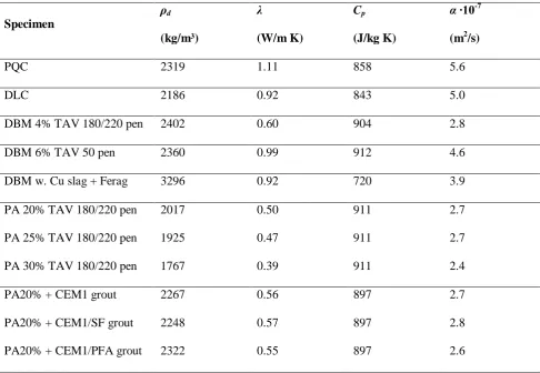
Results 185
The experimental data for the dry-state thermo-physical properties of these pavement materials is 186
presented in Table 3. DBM materials generally have a similar Volumetric Heat Capacity (VHC) to 187
Portland concrete but with lower thermal conductivity, due to the bituminous binder, and as a result 188
are less thermally diffusive. The high porosity (low density) of PA materials significantly reduces both 189
the thermal conductivity and thermal diffusivity, and the addition of cementicious grout gives an 190
increase in VHC without significantly affecting diffusivityor conductivity.The use of high density 191
alternative aggregates can significantly increase the VHC whilst maintaining a similar thermal 192
conductivity. 193
3. Predictive modelling of pavement temperature depth profiles 195
Since roadways represent a relatively large surface area, by neglecting edge effects the predictive 196
model can be reduced to a one-dimensional transient conduction model combined with a surface 197
energy balance approach to predict the surface temperature under given climatic variables. This simply 198
requires the cross-sectional construction detail of the pavement and the thermo-physical properties of 199
the materials to be known. In reality, the heat transport mechanisms in pavement materials (concrete, 200
asphalt or macadam) are complex, as depicted in Figure 1, and can involve radiation between particles, 201
convection in the pores, phase change processes (latent energy transport) vaporisation and 202
condensation process as well as freeze-thaw processes. Since pore sizes are negligibly small in relation 203
to the volume of the structure under consideration, satisfactory modelling predictions can be made by 204
reducing the complex heat transfer process to an equivalent conduction-only term (Brandl 2005). 205
206
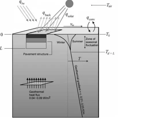
The factors influencing the pavement surface energy balance, as well as the heat transport processes 207
that occur within a pavement, are illustrated in Figure 2. The absorbed solar radiation on the pavement 208
surface, qabsorbedis simply equal to a∙qsolar, where „a‟ is the absorptivity coefficient. The sensitivity of 209
surface radiation absorption to pavement thermo-physical properties is dealt with in more detail in 210
Section 4. Thermal (long-wave) radiation heat flux between the pavement surface and surrounding 211
matter (i.e. the lower atmosphere, other buildings/objects) can be calculated as (Incropera et al. 2007): 212
213
4
0 4
εσT T
qthermal surr Eq. 1
214 215
Tsurr is a hypothetical temperature that collectively represents the notional temperature of the 216
surroundings objects and the lower atmosphere (air, clouds/water vapour), to which the surface can 217
radiate heat. In the absence of dew point temperature data (Tdp), Tsurr can be assumed as 6 K below the 218
ambient dry bulb air temperature (Underwood & Yik 2004, Lienhard & Lienhard 2006). Despite that 219
Tair≠ Tsurr some researchers have used the ambient air temperature alone to calculate long-wave 220
modelling tool for this work uses the empirical Bliss equation which estimates the surrounding 222
conditions in the form of a hypothetical „sky temperature‟ (an approximation of Tsurr) where (Gui et al. 223
2007, Chiasson et al. 2000, Yavuzturk et al. 2005): 224
225
Eq. 2 226
227
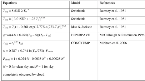
There are also many empirical models that attempt to improve on the accuracy of the Bliss equation. 228
The model in this paper was assessed using the empirical equations listed in Table 4. Figure 3 clearly 229
shows that over a representative three-day period, when compared to the LTPP experimental data, 230
using the Bliss equation gives the most accurate results and so this was used throughout the rest of the 231
study. 232
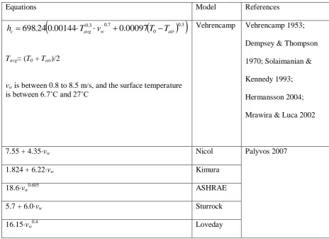
233
Convection (natural and forced) accounts for heat transport at the pavement surface and the heat flux 234
is simply calculated from qconvection = hc (Tair– T0 ). The disparity between mean air velocity and
near-235
surface air velocity, as a result of friction and uneven/rough surfaces, is often overlooked. The 236
modelling tool for this work uses the empirical Jurges equation which estimates the mean convection 237
heat transfer coefficient as a function of wind speed where (Niro et al. 2009, Bentz, 2000, CIBSE 238
2006): 239
240
hc = 5.8 + 4.1·vw Eq.10
241
There are also many empirical models used by other researchers in order to calculate convective heat 242
transfer at the pavement surface. The model in this paper was assessed using several other empirical 243
equations as listed in Table 5 and a direct comparison between surface temperature predictions and 244
LTPP experimental monitoring data has been performed. Figure 4 clearly shows that the Jurges‟ 245
estimation of hc provides the greatest level of accuracy over a representative 3-day period in two 246
contrasting climatic regions. This also suggests that surface convection heat transfer plays an 247
important role in near-surface temperature profile formation. 248
249
One-dimensional vertical heat transport by transient conduction through the pavement can simply be 250
modelled as a response to absorbed/desorbed energy at the pavement surface using an explicit form of 251
the finite difference (FD) method. The cross-sectional pavement profile and the sub-soil beneath it can 252
therefore be considered as a semi-infinite medium extending downward from d = 0 (pavement surface) 253
to d = x, at which point ΔT → 0. In reality, at a critical depth (usually several meters) the ground 254
temperature is approximately constant as a result of thermal mass and so is largely unaffected by 255
heating/cooling cycles at the pavement surface. The numerical solution to the boundary condition at 256
the pavement surface is then given by (Gui et al. 2007, Mrawira & Luca 2002): 257 258
d T T T T T T h q t T T d c i i sky i air c solar i i p d 0 1 4 0 4 0 0 10 a εσ
2
Eq. 3
259
260
The left side of Equation 3 gives the change in absorbed heat energy as a function of time, whilst the 261
right hand side components (from left to right) represent heat energy from short-wave (solar) radiation 262
gains, air convection gains/losses, long-wave radiation gains/losses, and fabric thermal conduction 263
to/from d = 0. For interior nodes, the rate of heat conduction across a volume element of thickness Δd 264
equals the change in the energy content of the element during a time interval Δt, therefore: 265 266 d t T T c d T T d T
T i m im
p d m i m i m i m i
1
1
1
Eq. 4267
268
A schematic diagram to identify the locations of mth node, m+1th node etc is shown in Figure
269
im im im
im im T T T T
d t
T
1 1 2 1 2
Eq. 5 272 273 where p dc
, the thermal diffusivity. The temperature of the interface nodes between layers of 274the pavement structure, e.g. the contact between surface layer and base layer, was derived from 275
Equation 4 to give: 276 277 2 2 2 1 2 2 1 1 1 1 2 1 2 1 1 1 d t T T c d t T T c d T T d T
T i m im
p d m i m i p d m i m i m i m i
Eq. 6278
279
This can then be solved for
T
i
1
m
to give: 280 281 t d c d c T t d c t d c d d T d T d T p d p d m i p d p d m i m i m i 2 2 2 2 2 2 1 1 1 2 2 2 1 1 1 2 2 1 1 1 2 2 1 1 1 1 Eq. 7 282 283The explicit method is not unconditionally stable, and the largest permissible value for the time step is 284
limited by a stability criterion. In the case of transient one-dimensional heat conduction, the upper 285
limit for all interior nodes is given by (Incropera et al. 2007, Holman 2002): 286
287
∆t≤ 0.5∆d2 /α Eq.8
288
In order to find the most restrictive value for ∆t, first a value for ∆d must be considered and then the 293
maximum value of α (refer Tables 1 and 3) is inserted in Equation 8. In addition, the minimum value 294
for ρd and cp as well as a maximum logical value for hrad, hc, and λ have to be inserted in Equation 9.
295
The minimum (i.e. most restrictive) value for ∆t should be used to provide the solution. In this study 296
values of Δd=0.02mand of ∆t = 30s were found to provide satisfactory stability for the range of 297
typical thermo-physical properties in pavement materials (refer Tables 1 and 3) as well as climatic 298
data. 299
300
The initial condition at t = 0 assumes a constant uniform temperature distribution to a depth of 2 m. 301
Equations 5 to 7 are then solved by iteration in order to predicatively compute the temperature depth 302
profile evolution at a given time interval. The environmental input parameters required for the model 303
are hourly (or more frequently) solar irradiation, dry bulb air temperature, relative humidity (or dew 304
point temperature) and mean wind velocity. The inputs were interpolated linearly across the hour 305
period in order to achieve the 30 sec interval required for the model. In addition to surface absorptivity 306
and surface emissivity, the pavement material thermo-physical properties required can be chosen from 307
Tables 1 and 3 or experimentally determined. 308
309
4. Model sensitivity to pavement surface boundary conditions 310
The typical emissivity, ε, of concrete is 0.88 – 0.93 and for asphalt 0.85 – 0.93 (Incropera et al. 2007). 311
Absorptivity (a) of a surface is the fraction of solar energy that is absorbed by the surface and it is 312
normally a function of wavelength of the incoming radiation, surface colour, wetness, average 313
temperature of pavement, and age of pavement surface (Solaimanian & Kennedy 1993). The 314
absorptivity of a pavement surface generally decreases during its lifetime as the surface colour 315
becomes lighter, and the reduction is more profound in asphalt pavements due to the high 316
susceptibility of bitumen to aging (CIBSE 2006). For concrete pavement surfaces, „a‟ values as low as 317
0.60 have been reported (Incropera et al. 2007) with a typical range being 0.65 – 0.80 (Bentz 2000, 318
CIBSE 2006). Typical values for asphalt and macadam surfaces are 0.85 – 0.95 (Yavuzturk et al. 319
2005, CIBSE 2006). The values for pavement materials in general are lower than the typical range for 320
bare soil surfaces which are 0.85 – 0.92 (Holman 2002,Asaeda & Wake 1996). The relatively high 321
sensitivity of near-surface temperature predictions to changes in „a‟ can be seen in Figure 6 where the 322
typical range in „a‟ values for conventional pavement materials (concrete, asphalt and macadam) were 323
used in the FD model and compared with LTPP experimental monitoring data. The highest solar 324
irradiation test region (i.e. Arizona) was used in order to demonstrate maximum sensitivity. It can be 325
seen that in this climate a difference of around 10 ˚C in the near-surface temperature could be 326
achieved for the pavement materials used in this study. Note that the assumed „a‟ value for this LTPP 327
pavement was 0.88 which gave a good agreement between the predicted values and the measured 328
values. 329
330
5. Temperature prediction and validation in different climatic regions 331
5.1 Validation against LTPP data 332
The FD model described earlier was used to predict pavement temperature profile evolution, at various 333
different depths, in response to the climatic variables period. This was compared with actual recorded 334
data provided by the SMP database of the LTPP project (US Department of Transportation – Federal 335
Transport Administration, 2009). Five regions of contrasting climate were selected across the USA, as 336
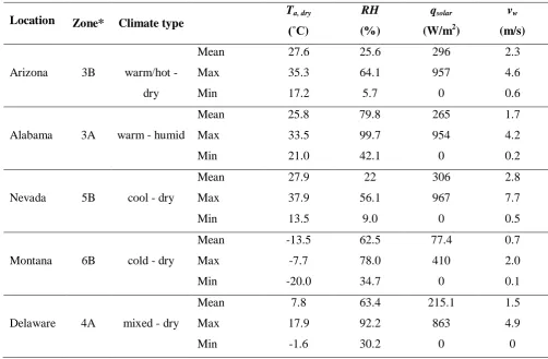
shown in Figure 7 along with the corresponding latitude and longitude. The climatic region and mean 337
climatic variables for each test site are summarised and compared in Table 6. The predicted 338
temperatures were modelled at three depth categories within the pavement; near-surface (<25mm), 339
sub-surface (70-150mm) and mid-depth (200-350mm). The precise value for d in each of the three 340
depth categories varied depending upon the precise position of the thermocouples at the five different 341
LTPP project locations, as shown by the cross-sectional construction details of the test pavements in 342
Figure 8. This shows the precise thermocouple location and thermo-physical material properties for 343
each layer. The default absorptivity values used in the modelling were 0.85 for asphalt and 0.65 for 344
concrete, taken as the mean average from published values (see above). For Arizona, the asphalt value 345
was increased to 0.88 to account for the application of a dark surface sealant referred to in the SMP 346
notes. In Montana, the concrete value was reduced to 0.60 to represent the formation of surface frost 347
sub-surface and mid-depth temperature profile evolution, and the actual SMP recorded data, was made 349
over a 3-day representative period for each of the five test locations detailed above, see Figures 9 – 13. 350
351
5.2 Comparison with Enhanced Integrated Climatic Model (EICM) 352
An important way to validate the model is to compare it to other well established tools already 353
available to industry and the scientific community. For this reason the authors have chosen to run two 354
analyses to compare the results from the Enhanced Integrated Climatic Model, implemented within the 355
Mechanistic-Empirical Pavement Design Guide (ME-PDG) with those of the presented model under 356
two climatic scenarios selected from the LTPP database, i.e. 1-0101 (Alabama) and 31-3018 357
(Montana). Some input parameters that are required for our model could not be specified in the ME-358
PDG user interface and could, therefore, slightly decrease the accuracy of the simulations. The values 359
used for these parameters were: Cloud Base Factor = 0.9, vapour pressure of air = 1.33mbar 360
(minimum of range), a = 0.98 (newly constructed road), and surface emissivity = 0.93. The average 361
daily values of air temperature, wind speed and pavement temperature with depth were all available in 362
the climatic database for these sections, while the percentage of sunshine was onlygiven as a monthly 363
average and therefore, for the sake of the simulation, values were interpolated on a daily scale. Figures 364
14 and 15 show a comparison between the estimation of average monthly temperature at various 365
depths (surface, 0.4m, 1m and 2m) performed using the two different models. The difference between 366
predicted values from our model and EICM (within ME-PDG) was found to be between a mean value 367
of 0.23˚C (Montana) and 0.55˚C (Alabama), which is less that the typical accuracy of a thermocouple 368
used to record the experimental values (~ +/- 0.5˚C). It is not possible to directly compare the 369
computational time for the two models in a fair way, since the ME-PDG must also perform structural 370
analysis of the pavements as well as the thermal simulation, which requires several minutes 371
(approximately 10 minutes for each of these simulations), whilst our model is coded in C# and can run 372
the same simulations in less than one second. 373
374
The model presented here is intended to function as a simple research tool and performs to an 375
acceptable standard and is typically accurate to within a 2 ˚C variation about the LTPP recorded 376
experimental value in all cases. This is at least the same level of accuracy as has been achieved in 377
previous attempts to model pavement temperature profile evolution using a 1D transient conduction 378
approach with dry state material thermo-physical properties (Dempsey & Thompson 1970, Rosenfeld 379
et al. 1998, Solaimanian & Kennedy 1993, Hermansson 2000, Hermansson 2004), as well as when 380
employing a 2-D FD model (Yavuzturk et al. 2005) and when using a 3D ANSYS FE model (Minhoto 381
et al. 2006). The fast, simple, and computationally efficient Finite Difference (FD) approach was 382
chosen for this study to enable rapid comparisons between multiple sets of material thermo-physical 383
parameters and climatic variables without having to perform a detailed pavement structural design 384
before each simulation, as with the EICM (ME-PDG). A hygrothermal (coupled heat & moisture) 385
model would require extensive and detailed material properties characterisation for input parameters in 386
terms of moisture-dependent thermal conductivity, moisture-dependent heat capacity, 387
sorption/desorption isotherms, vapour permeability and liquid permeability coefficients. Pavement 388
materials are non-homogenous and often only limited historical thermo-physical data (or core sample 389
extraction) for existing highways is available. The authors propose that, given the accuracy of our 390
simple model which requires only dry-state thermo-physical properties and climatic data and the scale 391
of the pavement structure (thickness) and given the small additional accuracy gained from a 392
hygrothermal modelling approach, that the research objective is very well satisfied without it. 393
394
6. Sensitivity analysis on the influence of material thermo-physical properties 395
Two categories were identified in order to define the „thermal response‟ of a pavement structure to its 396
ambient climatic conditions, in order to evaluate its sensitivity to changes in the material thermo-397
physical properties: 398
o Cyclic peak temperature variation as a function of depth (maximum/minimum) 399
o Amplitude suppression and time lag of peak temperature occurrence as a function of 400
depth 401
402
For each category, the objective of the analysis was to determine how the controlled variation, for each 403
of the achievable thermo-physical properties of pavement materials, can dominate any specific 404
changes in thermal response, and to what extent the magnitude of those changes are climate-specific. 405
The outcomes of this analysis can be conveniently summarised under three sets of general 406
conclusions, corresponding to the data presented in Figures 16 – 18. 407
408
Near-surface (0 – 25mm) peak temperatures and the range of peak temperature fluctuation (in a daily 409
cycle) is inversely related to the thermal conductivity of the pavement surface layer, whilst at the same 410
instance, mid-depth pavement temperatures are positively related, as shown by Figure 16. This 411
behaviour occurs because heat flux away from the hot pavement surface (or from a hotter pavement 412
core to a cooler surface) is increased when λ is high in the surface layer. The effect is greatest where 413
surface energy gain is high, e.g. typically when short-wave or long-wave radiation gains, or 414
convection gains, are high. We therefore see the greatest gains in Arizona and Nevada (up to 5˚C 415
reduction in maximum , or 3˚C increase in minimum), a lesser extent in the humid/temperate climates 416
of Alabama and Delaware (1˚C reduction in maximum, 2˚C increase in minimum), and only minimal 417
changes in Montana (1˚C increase in minimum). Chen et al. (2008) used the NCHRP 1-37A 418
Mechanistic Empirical Pavement Design Guide (ME-PDG) in order to show the relationship between 419
pavement service life and maximum pavement surface temperature. They showed that, for the same 420
traffic and the same materials, the life of the pavement can be extended by five years for a drop in 421
temperature of 5°C. The opposite is true when low λ values are used, when surface temperatures are 422
increased and mid-depth is decreased. In either case, separate analyses showed no significant effect on 423
the time at which peak temperatures occur, i.e. no phase shift. 424
425
The VHC is positively related to the overall range of daily cycle temperature fluctuation and time-426
dependency of peak temperature occurrence, i.e. it governs the response time and sensitivity of 427
material temperature to changes in the surface energy fluxes. Obviously the magnitude of peak 428
temperature suppression about the mean (as a function of time) is directly proportional to diurnal 429
temperature fluctuation, and largely independent of the mean temperature itself, as can be seen in 430
Figure 17. Therefore, up to 4˚C suppression in maximum temperature is achievable in Delaware (~ 431
30˚C diurnal range), compared to only around 1˚C suppression in Montana (~ 12˚C diurnal range). In 432
all cases, the time lag in occurrence of both maximum and minimum peak temperatures is 433
approximately 1 hour longer for the high VHC surface layer materials compared with those of low 434
VHC. This suggests that whilst significant potential exists for optimising pavement surface layer 435
materials in order to buffer peak temperatures, there is little potential for displacing the peak heat 436
output relative to peak input time, e.g. so as to effect a reduction in urban temperatures during working 437
hours. 438
439
The critical depth (dcrit) is defined by the point of convergence in daily cycle maximum/minimum 440
temperature profiles and, from previous research conducted by the authors, is known to be positively 441
related to the thermal diffusivity of pavement materials (Keikha et al. 2010). The implications are that 442
the depth at which temperature stability is achieved can be controlled by layer thickness and material 443
specification. For low diffusivity pavement surface materials, dcrit is approximately between 100 and 444
150mm regardless of climate, as shown by Figure 18. For high diffusivity pavement surface materials, 445
dcrit is between, approximately, 250 and 400mm. It appears that dcrit is positively related to both the 446
thermal diffusivity and thickness of the surface layer, and largely independent of climatic variables. 447
Diffusivity simply represents the time-variant spread of heat energy and so determines the position at 448
which temperature stability occurs in a pavement slab. 449
450
7. Conclusions and practical applications 451
It is concluded that various improvements can be made at the design stage of transport infrastructure 452
by understanding the implications of the interaction between pavement design, the thermo-physical 453
properties of the specified materials, and the ambient climatic conditions. Rutting is a particular 454
problem in asphalt/macadam materials since they have a temperature-dependent Young‟s Modulus 455
binder, i.e. they are bitumen-based. The ability to reduce surface temperatures in climates with high 456
peak temperatures and short-wave radiation gains might be highly beneficial. In general terms, a 457
pavement surface with high conductivity and low absorptivity will be cooler, as confirmed by our 458
numerical predictions and the LTPP experimental data, and therefore less likely to suffer from rutting. 459
Previous studies have also shown that when the maximum surface temperature is reduced by around 460
5ºC in hot climates such as Arizona and Nevada, the pavement service life can potentially be extended 461
by up to five years. The same approach could be used to counteract the urban heat island effect as it 462
would reduce heat emitted to the urban environment from the warm pavement surfaces, which is 463
typically transported by long-wave radiation and natural convection. 464
465
A numerical modelling tool of 1D transient thermal conduction has been presented for predicting 466
temperature profile evolution on pavement structures. It has been well validated in five contrasting 467
climatic regions using accepted long-term monitoring data from the SMP programme as part of the 468
LTPP project, and is as accurate as the best of comparable existing models. To improve prediction 469
accuracy beyond 2˚C would require a hygrothermal model (fully coupled heat and moisture 470
transport/storage) which necessitates highly detailed characterisation of the pavement material 471
properties. In the longer term, the influence of moisture transport and storage on the model accuracy 472
and climate-dependent response should be investigated to determine the influence on prediction 473
accuracy in high rainfall regions. In these scenarios the simple model is unlikely to fully reflect the 474
actual thermal processes of convection, radiation, and evaporation at the pavement surface, nor to 475
accurately model heat and moisture movement inside the pavement. However, comparisons with 476
models that do this, suggest that there is no significant improvement in accuracy for the wide range of 477
contrasting climatic conditions tested in this study. A simple tool like this is easily used and applied by 478
industry as part of pavement design protocol and material mix design specifications. 479
480
Warping usually effects rigid pavement layers, e.g. concrete surfaces or base layers, and is caused by 481
the formation of a high temp gradient across the layer. This could be overcome by adjusting thermal 482
diffusivity and therefore re-positioning the critical depth at a point immediately below the effected 483
layer. Expansion and contraction cracking is a similar issue but is more likely in climates with very 484
high diurnal temperature fluctuations, typically accompanied by high short-wave radiation gains at 485
peak temperatures. By increasing the VHC of the surface layer to give, say, 3-4˚C temperature 486
suppression (at peak) and around 6˚C reduction in total diurnal fluctuation (as demonstrated by the 487
data presented here) the issue of cracking and loss of strength caused by thermal expansion/contraction 488
could be significantly reduced. In cold climates, the ability to prevent the pavement materials from 489
getting so cold would be likely to have a measurable effect on extending fatigue life. In very cold 490
climates a thick, low diffusivity pavement surface layer could provide a more stable temperature at 491
shallower depths and thus reduce the freeze-thawing cycle and improve the pavement stability beneath 492
the surface, i.e. reducing intermittent thaw softening (a problem that is expected to increase 493
significantly in many northern climates as global warming prevents seasonal pavement freezing and 494
leads to multiple freeze-thaw cycles). Further research is needed to see how pavement design and 495
materials selection can be tailored to a specific location given the climatic variables of that region. Of 496
course, benefits of reduced rutting and extended fatigue life will only be realized for materials having 497
the same temperature susceptibility to these damage mechanisms. Much more work is required to 498
balance mechanical properties and thermal properties – a balance that will need to be determined in a 499
climate-specific framework. 500
501
Acknowledgements 502
The authors wish to acknowledge the financial support of this research by the Engineering and 503
Physical Sciences Research Council (EPSRC) and East Midlands Airport. In addition, the authors 504
wish to thank Robert Armitage and Daru Wityakamoto of the Scott Wilson Company, and Ayumi 505
Hatakeyama, Dr David Allinson, and Peter Phillips at the University of Nottingham for their technical 506
support, input and advice. 507
509
Table 1 – Previously published data for thermo-physical properties of pavement materials (dry state) 510
Specimen ρd (kg/m³)
λ (W/m K)
Cp (J/kg K)
α ∙10-7 (m2/s) Plain concrete (general) a, m 1600 - 3000 0.50 – 4.00 800 - 1200 1.4 - 20.8 Sub-soil (general) d 1400 - 2000 0.30 – 2.00 800 - 1100 1.4 - 17.8
PQC (general) 2339 e 1.20 a 1000 a 5.1
Crushed gravel/hardcore 2190 -2403 e 1.10 b 1000 c 4.6 - 5.0
Soil-aggregate mix 1650 e 1.00 b 960 d 6.3
Sub-soil 1782 -1906 e 0.80 d 1040 d 4.0 - 4.3
HMA f – l 1800 - 2500 0.50 - 2.50 900 - 2000 1.2 - 16.8
511 a
(Mehta and Monteiro 2006), b (Côté & Konrad 2005), c (Dempsey & Thompson 1970), d (ASHRAE 1995), e 512
(US Department of Transportation – Federal Transport Administration 2009), f (Luca & Mrawira 2005), g 513
(Solaimanian & Bolzan 1993), h (Mrawira & Luca 2006), i (Mrawira & Luca 2002), j (Gui et al. 2007), k 514
(Chadbourn et al. 1996), l (Zapata & Houston 2008), m (Lamond & Pielert 2006) 515
517
Table 2 – Aggregate type percentage passing from sieve analysis 518
Sieve size (mm)
14mm 10mm 6mm dust Filler
28 100 100 100 100 100
20 100 100 100 100 100
14 89.1 100 100 100 100
10 21.8 87.5 100 100 99.2
6.3 7 16.6 84.2 100 99.1
3.25 5.5 7.1 13.7 97.1 98.9
2.36 4.9 5.8 10 87.3 98.9
1.18 4.1 4.6 7.8 60.8 98.7
0.60 3.8 4.1 6.6 40.7 98.5
0.212 3 3 5.1 22.3 98
0.075 0.8 0.9 2.3 12.2 92.6
520
Table 3 – Thermo-physical properties of pavement materials (dry state) 521
Specimen
ρd
(kg/m³)
λ
(W/m K)
Cp
(J/kg K)
α ∙10-7
(m2/s)
PQC 2319 1.11 858 5.6
DLC 2186 0.92 843 5.0
DBM 4% TAV 180/220 pen 2402 0.60 904 2.8
DBM 6% TAV 50 pen 2360 0.99 912 4.6
DBM w. Cu slag + Ferag 3296 0.92 720 3.9
PA 20% TAV 180/220 pen 2017 0.50 911 2.7
PA 25% TAV 180/220 pen 1925 0.47 911 2.7
PA 30% TAV 180/220 pen 1767 0.39 911 2.4
PA20% + CEM1 grout 2267 0.56 897 2.7
PA20% + CEM1/SF grout 2248 0.57 897 2.8
PA20% + CEM1/PFA grout 2322 0.55 897 2.6
523
Table 4 - Models used to calculate thermal (long-wave) radiation heat flux 524
Equations Model References
Tsky = 5.53E-2·T0 1.5
Swinbank Ramsey et al. 1981
Tsky = (-3.015E9 + 1.22·T04)0.25 Swinbank Ramsey et al. 1981
Tsky = T0(1 - 0.261·exp(-7.77E-4(273-T0) 2
))0.25 Idso & Jackson Ramsey et al. 1981
q=εσ(4.8 + 0.075(Tair - 5))(T0 - Tair) HIPERPAVE McCullough & Rasmussen 1998
Tsky = εs0.25·Tair
εs = 0.787 + 0.764·ln(Tdp/273) ·Fcloud
Fcloud = 1+ 0.024·N - 0.0035·N2 + 0.00028·N3
N = 0 for clear sky and N = 1 for sky completely obscured by cloud
CONCTEMP Minhoto et al. 2006
527
Table 5 - Models used to calculate convective heat flux at pavement surface 528
Equations Model References
0.3
0 7
. 0 3 . 0
00097
.
0
00144
.
0
24
.
698
avg w airc
T
v
T
T
h
Tavg= (T0 + Tair)/2
vw is between 0.8 to 8.5 m/s, and the surface temperature is between 6.7˚C and 27˚C
Vehrencamp Vehrencamp 1953; Dempsey & Thompson 1970; Solaimanian & Kennedy 1993; Hermansson 2004; Mrawira & Luca 2002
7.55 + 4.35·vw Nicol Palyvos 2007
1.824 + 6.22·vw Kimura
18.6·vw0.605 ASHRAE
5.7 + 6.0·vw Sturrock
16.15·vw
0.4
Loveday
Table 6 – Mean climatic variables for the simulated test conditions in each of the five locations, data 532
sourced from LTPP SMP (US Department of Transportation – Federal Transport Administration, 533
2009) 534
Location Zone* Climate type Ta, dry (˚C)
RH
(%)
qsolar
(W/m2)
vw
(m/s)
Arizona 3B warm/hot - dry Mean Max Min 27.6 35.3 17.2 25.6 64.1 5.7 296 957 0 2.3 4.6 0.6
Alabama 3A warm - humid
Mean Max Min 25.8 33.5 21.0 79.8 99.7 42.1 265 954 0 1.7 4.2 0.2
Nevada 5B cool - dry
Mean Max Min 27.9 37.9 13.5 22 56.1 9.0 306 967 0 2.8 7.7 0.5
Montana 6B cold - dry
Mean Max Min -13.5 -7.7 -20.0 62.5 78.0 34.7 77.4 410 0 0.7 2.0 0.1
Delaware 4A mixed - dry
Mean Max Min 7.8 17.9 -1.6 63.4 92.2 30.2 215.1 863 0 1.5 4.9 0 535
Figure captions 538
Figure 1 – heat transport mechanisms between binder-coated aggregate particles, adapted from (Yun 539
& Santamarina 2008) 540
Figure 2 – cross-sectional illustration of ground heat fluxes and surface energy balance, adapted from 541
(Banks 2008) 542
Figure 3 – sensitivity comparison for long-wave radiation heat flux empirical formulae 543
Figure 4 – sensitivity comparison for near-surface temperature approximations due to convective heat 544
transport 545
Figure 5 – a schematic diagram to identify the locations of mth node, m+1th node etc used in the finite 546
difference model 547
Figure 6 – sensitivity comparison for near-surface temperature approximations under the range of 548
pavement material absorptivity values 549
Figure 7 – regional climatic map of the USA showing the selected LTPP test site locations, adapted 550
from (ASHRAE 2007). The two numbers given for each label are the latitude and longitude, 551
respectively. 552
Figure 8 – cross-sectional designs of the five selected LTPP test pavement structures 553
Figure 9 – Three-day model validation for near-surface, sub-surface and mid-depth temperature profile 554
evolution against LTPP experimental data for the Arizona test site 555
Figure 10 – Three-day model validation for near-surface, sub-surface and mid-depth temperature 556
profile evolution against LTPP experimental data for the Alabama test site 557
Figure 11 – Three-day model validation for near-surface, sub-surface and mid-depth temperature 558
profile evolution against LTPP experimental data for the Montana test site 559
Figure 12 – Three-day model validation for near-surface, sub-surface and mid-depth temperature 560
profile evolution against LTPP experimental data for the Nevada test site 561
Figure 13 – Three-day model validation for near-surface, sub-surface and mid-depth temperature 562
profile evolution against LTPP experimental data for the Delaware test site 563
Figure 15 – Comparison between simulated LTPP data (Alabama) using our model and the ME-PDG 566
EICM 567
Figure 16 – The influence of high and low thermal conductivity pavement surface layers on 568
temperature as a function of depth in each of the five test locations 569
Figure 17 – The influence of high and low volumetric heat capacity pavement surface layers on 570
temperature as a function of time in each of the five test locations 571
Figure 18 – The influence of high and low thermal diffusivity pavement surface layers on temperature 572
depth profile and critical depth in each of the five test locations 573
References 575
1. Asaeda, T. and Wake, V.T.C., (1996). “Heat Storage of Pavement and its Effect on the Lower 576
Atmosphere.” Atmospheric Environment, 30(3), 413-427. 577
2. ASHRAE, (2007). “ASHRAE Standard 90.1-2007 Energy Standard for Buildings Except Low-578
Rise Residential Buildings.” American Society of Heating, Refrigeration and Air Conditioning 579
Engineers Inc, Atlanta. 580
3. ASHRAE, (1995). “Commercial/institutional ground source heat pump engineering manual.” 581
American Society of Heating, Refrigerating and Air-Conditioning Engineers Inc, Atlanta. 582
4. Banks, D., (2008). “An Introduction to Thermogeology: Ground Source Heating and Cooling.” 583
Blackwell Publishing, Oxford. 584
5. Bentz, D. P., (2000). “A Computer Model to Predict the Surface Temperature and Time of 585
Wetness of Concrete Pavements and Bridge Decks.” NISTIR 6551, United States Department of 586
Commerce, USA. 587
6. Brandl, H., (2005). “Energy Foundations and other thermo-active ground structures.” 588
Geotechnique, 56(2), 81-122. 589
7. Bretz, S., Akbari, H. and Rosenfeld, A. H., (1998). “Practical Issues for Using Solar-Reflective 590
Materials to Mitigate Urban Heat Islands.” Atmospheric Environment, 32(1), 95-101. 591
8. BSI, (2005). “BS 4987-1:2005 Coated Macadam (Asphalt Concrete) for Roads and Other Paved 592
Areas - Specification for Constituent Materials and for Mixtures.” British Standards Institute, 593
London. 594
9. BSI, (2002). “BS EN 12620:2002 Aggregates for Concrete.” British Standards Institute, London. 595
10. Carder, D. R., Barker, K. J., Hewitt, M. G., Ritter, D., and Kiff, A., (2007). “Performance of an 596
inter-seasonal heat transfer facility for collection, storage, and re-use of solar heat from the road 597
surface.” Transport Research Laboratory (TRL), Published Project Report PPR 302. 598
11. CES Edupack, (2007). “Cambridge Engineering Selector: Materials and Processes Database” 599
[software], Granta Design, Cambridge 600
12. Chadbourn, B. A., Luoma, J. A., Newcomb, D. E., and Voller, V. R., (1996). “Consideration of 601
Hot-Mix Asphalt Thermal Properties During Compaction.” STP 1299 American Society for 602
Testing and Materials (ASTM), Philadelphia, 127–146. 603
13. Chen, B. L., Bhowmick, S., and Mallick, R. B., (2008). “Harvesting Energy from Asphalt 604
pavements and reducing the heat island effect”. Draft-2, White Paper-1. Available online at: 605
http://users.wpi.edu/~rajib/Draft-2White-Paper-on-Reduce-Harvest-Heat-from-Pavements-Nov-606
2008.pdf. 607
14. Chiasson, A. D., Spitler, J. D., Rees, S. J., and Smith, M. D., (2000). “A Model for Simulating the 608
performance of a Pavement Heating System as a Supplemental Heat Rejecter with Closed-Loop 609
Ground-Source Heat Pump Systems.” J. Solar Energy Eng., 122(4), 183–191. 610
15. Choubane, B. and Tia, M., (1992). “Nonlinear Temperature Gradient Effect on Maximum 611
Warping Stresses in Rigid Pavements.” Transportation Res. Record: J. Transportation Res. 612
Board, 1370, 11–19. 613
16. CIBSE, (2006). “Guide A: Environmental design – 7th Edition.” Chartered Institute of Building 614
Services Engineers, London 615
17. Côté, J. & Konrad, J. M., (2005). “Thermal Conductivity of Base-Course Materials.” Canadian 616
Geotechnical Journal, 42(2), 443-458. 617
18. Daiutolo, H., (2003). “Control of Slab Curling in Rigid Pavements at the FAA National Airport 618
Pavement Test Facility (NAPTF).” Available online at: 619
http://www.airtech.tc.faa.gov/NAPTF/Downloads/CC2%20Curling%20APT08.pdf. 620
19. de Bondt AH., (2003). “Generation of Energy Via Asphalt Pavement Surfaces.” Asphaltica 621
Padova, Netherland, Available online at: 622
http://www.roadenergysystems.nl/pdf/Fachbeitrag%20in%20OIB%20%20de%20Bondt%20-623
%20English%20version%2013-11-2006.pdf. 624
20. Defence Estates, (2006). “A Guide to Airfield Pavement Design and Evaluation – 2nd Edition.” 625
Ministry of Defence: Defence Estates, Sutton Coldfield. 626
22. Dempsey, B. J. & Thompson, M. R., (1970), “A Heat-Transfer Model for Evaluating Frost Action 629
Temperature-Related Effects in Multilayered Pavement System.” Transportation Res. Record: J. 630
Transportation Res. Board, 342, 39–56. 631
23. Densit a/s, (2000). Densiphalt® Handbook, Aalborg, Denmark. 632
24. Diefenderfer, B. K., Al-Qadi, I. L. and Reubush, S. D., (2002). “Prediction of Daily Temperature 633
Profile in Flexible Pavements.” Presented at Transportation Research Board 81st Annual Meeting, 634
Washington DC, January 2002. 635
25. Gui, J., Phelan, P. E., Kaloush, K. E., and Golden, J. S., (2007). “Impact of Pavement 636
Thermophysical Properties on Surface Temperatures.” J. Mater. in Civil Eng., 19(8), 683–690. 637
26. Hall, M. & Allinson, D., (2008a). “Assessing the Effects of Soil Grading on the Moisture Content-638
Dependent Thermal Conductivity of Stabilised Rammed Earth Materials.” Applied Thermal 639
Engineering 29(4), 740 – 747. 640
27. Hall, M. & Allinson, D., (2008b). “Assessing the Moisture-Content Dependent Parameters of 641
Stabilised Earth Materials Using the Cyclic-Response Admittance Method.” Energy and Buildings 642
40(11), 2044 – 2051. 643
28. Hermansson, A., (2004). “Mathematical Model for Paved Surface Summer and Winter 644
Temperature: Comparison of Calculated and Measured Temperatures.” Cold Regions Science and 645
Technology, 40, 1-17. 646
29. Hermansson, A., (2000). “Simulation Model for Calculating Pavement Temperatures, Including 647
Maximum Temperature.” Transportation Research Record, 1699, 134-141. 648
30. Holman, J. P., (2002). “Heat Transfer.” McGraw-Hill, New York. 649
31. Hunter, R. (Ed.), (2003). “The Shell Bitumen Handbook.” Thomas Telford, London. 650
32. Incropera, F. P., DeWitt, D. P., Bergman, T. L. and Lavine, A. S., (2007). “Fundamentals of heat 651
and mass transfer - 6th edition.” John Wiley & Sons, USA. 652
33. ISO, (1996). “8301: 1996 Thermal Insulation – Determination of Steady-State Thermal Resistance 653
and Related Properties – Heat Flow Meter Apparatus.” International Organization for 654
Standardization, Genève, Switzerland. 655
34. Keikha, P., Hall, M. R., and Dawson, A. R., (2010). “Concrete pavements as a source of heating 656
and cooling.” Proceedings for the 11th
International Symposium on Concrete Roads, 13th – 15th 657
October, Seville, Spain. 658
35. Lamond, J. F. & Pielert, J. H. (Eds.), (2006). “Significance of Tests and Properties of Concrete 659
and Concrete-Making Materials.” ASTM STP 169D, West Conshohocken, PA, USA. 660
36. Lienhard, I. V. and Lienhard, V., (2006). “A heat transfer text book.”Phlogiston Press, 661
Cambridge. 662
37. Luca, J. & Mrawira, D., (2005). “New Measurement of Thermal Properties of Superpave Asphalt 663
Concrete.” J. Mater. Civil Eng., 17(1), 72–79. 664
38. Marshall, C., Meier, R. W., and Welsh, M., (2001). “Seasonal Temperature Effects on Flexible 665
Pavements in Tennessee.” Presented at Transportation Research Board 80th Annual Meeting, 666
Washington DC, January 2001. 667
39. McCullough, B. F. & Rasmussen, R. O., (1998). “Fast track paving: concrete temperature control 668
and traffic opening criteria for bonded concrete overlays Volume I - Final Report.” Technical 669
Report, Federal Highways Administration, VA, USA. 670
40. Mehta, P. K. & Monteiro, P. J. M., (2006). “Concrete: Microstructure, Properties, and Materials – 671
Third Edition”, McGraw-Hill, USA. 672
41. Minhoto, M. J. C., Pais, J. C., Pereira, P. A. A., and Picado-Santos, L. G., (2006). “Predicting 673
asphalt pavement temperature with a three-dimensional finite element method.” Journal of the 674
Transportation Research Board, 96-110. 675
42. Mohseni, A. & Symons, M., (1998). “Improved AC Pavement Temperature Models from LTPP 676
Seasonal Data.” Presented at Transportation Research Board 77th Annual Meeting, Washington, 677
DC, January 1998. 678
43. Mrawira, D. & Luca, J., (2006). “Effect of aggregate type, gradation, and compaction level on 679
thermal properties of hot-mix asphalts.” Canadian. J. of Civil Engineering 33(11), 1410–1417. 680
44. Mrawira, D. & Luca, J., (2002). “Thermal Properties and Transient Temperature Response of Full-681
Depth Asphalt Pavements.” Transportation Res. Record: J. Transportation Res. Board, 1809 682
46. Niro, N., Shigenobu, M., Nishiwaki, M., and Takeuchi, M., (2009). “Numerical simulation of 684
snow melting on pavement surface with heat dissipation pipe embedded.” Heat Transfer - Asian 685
Res., 38(5), 313–329. 686
47. Palyvos, J. A., (2008). “A survey of wind convection coefficient correlations for building 687
envelope energy systems‟ modelling.” Applied Thermal Engineering, 28, 801-808. 688
48. Ramadhan, R. H. & Wahhab, H. I. A., (1997). “Temperature variation of flexible and rigid 689
pavements in eastern Saudi Arabia.” Building and Environment, 32(4), 367-373. 690
49. Ramsey, J. W., Chiang, H. D., and Goldstein, R. J., (1981). “A study of the incoming longwave 691
atmospheric radiation from a clear sky.” Journal of Applied Meteorology, 21, 566-578. 692
50. RETScreen, (2005). “Clean Energy Project Analysis: RETScreen Engineering & Cases 693
Textbook.” Minister of Natural Resources Canada, ISBN: 0-662-39191-8. 694
51. Rosenfeld, A. H., Akbari, H., Romm, J. J., and Pomerantz, M., (1998). “Cool Communities: 695
Strategies for Heat Island Mitigation and Smog Reduction.” Energy and Buildings, 28(1), 51-62. 696
52. Setyawan, A., (2003). “Development of Semi-Flexible Heavy-Duty Pavements” PhD thesis, 697
University of Leeds, UK. 698
53. Solaimanian, M. & Bolzan, P., (1993). “Analysis of the Integrated Model of Climatic Effects on 699
Pavements.” Technical report SHRP-A-637. 700
54. Solaimanian, M. & Kennedy, T. W., (1993). “Predicting Maximum Pavement Surface 701
Temperature Using Maximum Air Temperature and Hourly Solar Radiation.” Transportation 702
Research Record, 1417, 1-11. 703
55. Underwood, C. P. & Yik, F. W. H., (2004). “Modelling methods for energy in buildings.” 704
Blackwell publishing, Oxford. 705
56. US Department of Transportation – Federal Transport Administration, (2009). “LTPP Seasonal 706
Monitoring Programme (SMP): Pavement Performance Database (PPDB).” [electronic database], 707
Standard Data Release 23.0, DVD Version, USA. 708
57. van Bijsterveld, W. T. and de Bondt, A. H., (2002). “Structural Aspects of Asphalt Pavement 709
Heating and Cooling Systems.” Third International Symposium on 3D Finite Element Modelling, 710
58. Vehrencamp, J., (1953). “Experimental Investigation of Heat Transfer at an Air-earth Interface.” 712
Trans. Amer. Geophys. Union, 34, 22–29. 713
59. Yavuzturk, C., Ksaibati, K., and Chiasson, A. D., (2005). “Assessment of Temperature 714
Fluctuations in Asphalt Pavements Due to Thermal Environmental Conditions Using a Two-715
Dimensional, Transient Finite-Difference Approach.” J. Mater. in Civil Eng., 17(4), 465–475. 716
60. Yun, T. S. & Santamarina, J. C., (2008). “Fundamental Study of Thermal Conduction in Dry 717
Soils, Granular Matter.” 10(3), 197-207. 718
61. Zapata, C. E. & Houston, W. N., (2008). “Calibration and Validation of the Enhanced Integrated 719
Climatic Model for Pavement Design.” NCHRP Report 602, Transportation Research Board, 720
Washington, D.C. 721
Figure 1
Figure 2
Figure 3
Figure 4
Figure 5
Figure 6
Figure 7
Figure 8
Figure 9
Figure 10
Figure 11
Figure 12
Figure 13
Figure 14
Figure 15
Figure 16
Figure 17
Figure 18