PFClust : a novel parameter free clustering algorithm

algorithm

Mavridis

et al.

R E S E A R C H A R T I C L E

Open Access

PFClust: a novel parameter free clustering

algorithm

Lazaros Mavridis

, Neetika Nath

and John BO Mitchell

Abstract

Background:We present the algorithm PFClust (Parameter Free Clustering), which is able automatically to cluster data and identify a suitable number of clusters to group them into without requiring any parameters to be specified by the user. The algorithm partitions a dataset into a number of clusters that share some common attributes, such as their minimum expectation value and variance of intra-cluster similarity. A set ofnobjects can be clustered into any number of clusters from one ton, and there are many different hierarchical and partitional, agglomerative and divisive, clustering methodologies available that can be used to do this. Nonetheless, automatically determining the number of clusters present in a dataset constitutes a significant challenge for clustering algorithms. Identifying a putative optimum number of clusters to group the objects into involves computing and evaluating a range of clusterings with different numbers of clusters. However, there is no agreed or unique definition of optimum in this context. Thus, we test PFClust on datasets for which an external gold standard of‘correct’cluster definitions exists, noting that this division into clusters may be suboptimal according to other reasonable criteria. PFClust is heuristic in the sense that it cannot be described in terms of optimising any single simply-expressed metric over the space of possible clusterings.

Results:We validate PFClust firstly with reference to a number of synthetic datasets consisting of 2D vectors, showing that its clustering performance is at least equal to that of six other leading methodologies–even though five of the other methods are told in advance how many clusters to use. We also demonstrate the ability of PFClust to classify the three dimensional structures of protein domains, using a set of folds taken from the structural bioinformatics database CATH.

Conclusions:We show that PFClust is able to cluster the test datasets a little better, on average, than any of the other algorithms, and furthermore is able to do this without the need to specify any external parameters. Results on the synthetic datasets demonstrate that PFClust generates meaningful clusters, while our algorithm also shows excellent agreement with the correct assignments for a dataset extracted from the CATH part-manually curated classification of protein domain structures.

Background

In pattern recognition, data analysis is used for predicting the behaviour of an unseen test dataset. Amongst problems of this kind, two different types can be clearly distinguished. The first is supervised learning or classification, where a labelled training dataset with known categories is involved. The second kind is unsupervised learning or clustering, where no prior

information is available for grouping the dataset. The objective of a clustering algorithm is to partition the given data into mutually exclusive and meaningful [1] clusters; this can provide a better understanding of the natural structure of the data. Semi-supervised [2] classi-fication, which combines strategies from both supervised and unsupervised methods, has also grabbed attention in various fields of research as it requires less human ef-fort and gives better accuracy [3] than unsupervised learning. In this paper, we focus our attention on the challenges faced by clustering algorithms [4,5].

* Correspondence:[email protected]

†_{Equal contributors}

Biomedical Sciences Research Complex and EaStCHEM School of Chemistry, Purdie Building, University of St Andrews, North Haugh, St Andrews, KY16 9ST, Scotland, UK

There are numerous clustering algorithms discussed in the literature, traditionally clearly distinguished as either hierarchical [6] or partitional [7]. Hierarchical methods group the objects together layer by layer, based on the closeness of the data points as measured by suitable similarity or distance metrics. Hierarchical clustering se-quentially partitions the dataset, either by successively dividing an initial single cluster in divisive methods, or by joining together initially unlinked objects in agglom-erative algorithms. In a hierarchical method, once two objects are clustered together they remain together at all subsequent levels of the scheme with fewer clusters. Contrastingly, partitional clustering algorithms, such as k-means, do not have a layer by layer structure and ob-jects may sometimes move from one cluster to another.

The k-means method iteratively assigns each point to the cluster whose centroid is closest to it, recalculates the cluster centroids, and reassigns the points. This process continues until the assignments no longer change at each iteration. k-means tends to generate ap-proximately equally sized clusters, minimising intra-cluster distances; however, its preference for globular clusters and its failure to reproduce clusters of complex shape are limitations [5].

Determining the number of clusters

Automatically determining the number of clusters is a

major problem in clustering. A set of n objects can be

clustered into any numberkof clusters 1≤k≤nby any

of the methods we have discussed. Identifying the opti-mal number of clusters involves computing a range of

different numbers of clusters k, with the objective of

finding the best value of kthat gives the optimum

clus-tering. However, there is no agreed or unique definition of optimum in this context. Using internal and external

validation measures as described in Handlet al. [5], one

could design a protocol for reaching a decision on the

bestk. A gap statistic [8] addressed this issue by acting

as an internal validation measure, and has been applied in bioinformatics [9]. Though in principle it is not hard

to design a workflow to find the best k, in practice this

is not commonly done. This is partly because there is no consensus as to which of the many different possible measures should be used to compare clusterings with different numbers of clusters, a more difficult problem

than the comparison of clusterings with the samek. This

adds to the difficulty of choosing the best clustering method for finding the structure of a novel dataset.

Validation

Validation [4,8] plays an important role in deciding the number of clusters, as well as in assessing the perform-ance of the clustering algorithm. Cluster validation is designed to evaluate and compare clustering algorithms

by their ability to analyse a dataset. There are many different validation measures. Internal measures like Silhouette width [9] and Dunn Index [10,11] depend on the inherent structure of the data [12]. External mea-sures, such as the Rand Index [13] commonly used to evaluate the noise in biological data, depend on com-parison with an externally known gold standard classifi-cation of the objects.

Here we propose a novel clustering algorithm, PFClust

(Parameter Free Clustering), suitable for use where no

prior information about the number of clusters is given. As input, only similarity scores within the dataset are re-quired, and evaluation of the clustering is part of the

al-gorithm. A previous study by Akogluet al. [14] designed

a parameter free graph clustering algorithm to find co-hesive clusters, PICS. They have shown the efficiency of their method using real-world datasets including data from YouTube and Twitter. Our method shares the property of being parameter-free, but is aimed at classi-fying objects rather than graphs.

As the availability of biological information acceler-ates, it is necessary to find the natural structure or pat-terns in data in order to understand biological questions. In bioinformatics, grouping proteins based on sequence [1] or structure is a very common task. Classification of novel proteins [15] can be performed by using pattern recognition approaches, built on the assumption that some underlying characteristics are considered, while clustering proteins into superfamilies and families. There are numerous classification schemes for protein se-quences including PIR-PSD [16], a freely available data-base of protein sequence classification mostly applied for functional annotation, and Pfam [17], a classification of functional protein domains based on hidden Markov models and multiple sequence alignments.

Methods

Here we describe a partitional algorithm that uses the idea that each cluster can be represented as a non-predetermined distribution of the intra-cluster similar-ities of its members. The algorithm partitions a dataset into a number of clusters that share some common attri-butes, such as their minimum expectation value and variance of intra-cluster similarity. It is an agglomerative algorithm, meaning that it starts with separated objects and progressively joins them together to form clusters. PFClust is heuristic in the sense that it cannot be de-scribed in terms of optimising any single simply-expressed metric over the space of possible clusterings. Nonetheless, we demonstrate that, over a number of val-idations on test datasets, it produces clusterings that closely reflect the structure of the test data, and outper-forms many well established algorithms in this regard. We have taken a number of design decisions to optimize the algorithm with respect to time efficiency and result stability.

Since we represent each cluster as the distribution of the similarities between its members, we need to have a clustering criterion in order to separate different clusters and find the cluster structure. The criterion used in this algorithm is the expectation value of the similarity distri-bution between cluster members. In order to select a suitable threshold, we will need a good approximation to the distribution of mean intra-cluster similarities for all possible clusterings. We can then select the most appro-priate threshold value given an internal validation meas-ure. The number of unique clusterings for a dataset with

n points when we do not know the number of clusters,

O(n),a prioriis the Bell number:

o nð Þ ¼X n

k¼0

1

k!

Xk

j¼0 −1

ð Þk−j k j jn

where k is the number of clusters, inclusive of

single-tons. This number grows rapidly with the number of points in the dataset. Hence, instead of attempting an exhaustive search of all possible clusterings, we perform a random sampling, where we randomly decide the number of clusters and randomly assign the initial distri-bution of points amongst clusters. This sampling ap-proach is necessary for efficiency, but introduces a random element to the algorithm. In order to optimize some of our design decisions for the algorithm, we have internally validated using a synthetic dataset of 1500 two-dimensional (2D) vector points.

Algorithm

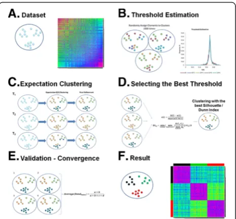
The clustering algorithm consists of two parts. The first part is the randomization, and the second part incorpo-rates both the threshold selection and the actual

clustering. Thus, in the first part (panel B of Figure 1),

20 thresholds are estimated (T1,…, T20) by a

randomization process. In the second part (panels C & D of Figure 1), each threshold is used to cluster the data, and the best threshold is selected. This whole process, incorporating both randomization and threshold selec-tion, is carried out four times (panel E of Figure 1). If the four resulting clusterings do not agree, the algorithm replaces the least successful of the four runs with a fresh attempt and repeats until convergence. Figure 1 shows a graphical representation of the clustering algorithm.

Threshold estimation

Given a dataset Ω = {α1,…,αn} with n members, the

threshold values are estimated by multiple random clus-terings of the data. Firstly, a random number of clusters

k(where1≤k≤n) is chosen and each data pointαis

ini-tially randomly placed in one of the clusters. Now letXi

be the distribution of the similarities between the

ele-ments of cluster i. The mean intra-cluster similarity,

which is the expectation value of the distribution Xi, is

defined so as to exclude self-similarities and can be cal-culated as:

E X½ ¼i

1

ni

2

Xni

j¼2

Xj−1

q¼1

sαj;αq

whereXiis the ith cluster,ni is the number of members

of that cluster and sαj;αq is the similarity between

elements αj and αq. In order to estimate an efficient

value for N, the number of randomizations used for

threshold estimation, we selected a dataset and simu-lated the randomization process. We repeated this ten

times for a number of different values of N. Figure 2

shows that using a small number of randomizations greatly affects the shape and sharpness of the

distribu-tion. However, increasingNgreatly affects the execution

time of the algorithm, since the randomization is the most expensive part of the calculation. Hence, as a

com-promise between accuracy and expense, we selectedN=

1000 as the number of randomizations, since this is the smallest number which gives an acceptably sharp distri-bution of mean cluster similarities. The

intra-cluster mean similarities, E[Xi], from every individual

cluster across the 1000 randomizations are collated into a single distribution. From this distribution, we retrieve 20 threshold values from the 95% - 100% significance levels, that is the 5% of the clusters with the highest mean intra-cluster similarities. We select the ten values corresponding to the following percentiles {95.00%, 97.50%, 99.00%, 99.14%, 99.29%, 99.43%, 99.57%, 99.71%, 99.86% and 100.00%} and ten further thresholds corre-sponding to the second to eleventh highest values in the distribution of intra-cluster similarities. Using this num-ber of thresholds provides a way of reducing the random element of our sampling.

Similarity-based clustering

Now, for each threshold valueT, the datasetΩ is

clus-tered with a similarity-based clustering. We begin with all elements separated and no clusters defined. The two

most similar elements inΩare placed together to form

the first cluster. For each of the (n-2) remaining

ele-ments, we compute its average similarityE[X] to the

el-ements already in cluster 1, and we now identify the element with the highest similarity. If this value is

lar-ger than T, the algorithm considers adding this most

similar element to the given cluster. The element is

added if and only if the element’s average similarity

compared to the members of that cluster is at leastP%

of T and the overall E[X] of the cluster is also larger

than T. This process is repeated until no new element

can be added to the cluster withoutE[X] of the cluster

falling below T. At this stage, a new cluster is formed

from the two most similar remaining elements,

pro-vided that their similarity exceeds T. This process is

continued iteratively until all elements of Ω have been

clustered, or until the remaining elements cannot form a cluster that has an expectation value of intra-cluster

simi-larity greater thanT.

The P% of Tcut-off was selected as a way to restrict

the intra-cluster variation of the similarities since, in a very tight cluster, outlier members could be included

because, even if they are distant from the other cluster

members, the totalE[X] could still be aboveT. In order

to estimate the value ofP, we performed a number of

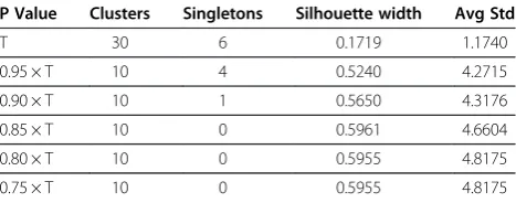
ex-periments on our dataset with differentP values. Table 1

shows the results, from which we see that a value ofP=

85% of Tgives the optimal results with respect to the

Silhouette width as well as the number of clusters, with multi-member clusters and singletons being shown separately.

After the data are assigned to clusters, a final refine-ment step is applied to all points that have an average

similarity score less thanTwhen compared to the

mem-bers of the cluster they have been assigned to. Each such point has its average similarity calculated with every cluster and is assigned to the cluster to which it is most similar (if this is not its original cluster, then the process moves the point to a different cluster; this assignment to

a cluster is made even if the point’s average similarity to

the members of its new cluster is less thanT).

Selecting the best threshold

For each of the 20 different T values, a clustering has

been obtained from the algorithm. For each of these clusterings, the mean Silhouette width (averaged over every point in the dataset) and the Dunn Index of the clustering are computed. The Silhouette width is defined

for each elementias:

s ið Þ ¼ b ið Þ−a ið Þ

maxfa ið Þ;b ið Þg

where a(i) is the average dissimilarity, where

dissimilar-ity is 1-similardissimilar-ity, of element i with all the other

ele-ments of the same cluster and b(i) the average

dissimilarity of elementito all the members of the

clos-est neighbouring cluster. In order to take singletons into

account, a negative score (−1) is given to each singleton

point in the proposed clustering. The Dunn Index is de-fined as:

DIm¼ min

1≤i≤m 1≤minj≤m;j≠i

δ Ci;Cj

max

1≤k≤mΔk

8 < : 9 = ; 8 < : 9 =

;∀i;j;k

where δ(Ci,Cj) is the inter-cluster distance between the

centres of clustersiandj, and max1≤k≤mΔkis the

0 0.02 0.04 0.06 0.08 0.1 0.12 0.14 0.16 0.18

0 0.21 0.41 0.61 0.81

Frequency %

E[X] Threshold Estimation

10 10^2 10^3 10^4 10^5

0 1 2 3 4 5 6 7 8 9

0 0.21 0.41 0.61 0.81

Number of Clus

te rs E[X] 10 Randomizations 0 10 20 30 40 50 60 70

0 0.21 0.41 0.61 0.81

Number of Clus

te

rs

E[X]

102_{Randomizations}

0 100 200 300 400 500 600 700

0 0.21 0.41 0.61 0.81

Nu mber of Cl usters E[X]

103Randomizations

0 1000 2000 3000 4000 5000 6000

0 0.21 0.41 0.61 0.81

Nu mber of Cl usters E[X]

104Randomizations

0 10000 20000 30000 40000 50000 60000

0 0.21 0.41 0.61 0.81

Number of

Clusters

E[X]

105_{Randomizations}

cluster and the cluster centroid. The cluster centroid is the element with the maximum similarity to the other members of the cluster. The Silhouette width is the main factor used in deciding which threshold produces the best clustering, and the Dunn Index is used only as a tie-breaker to decide cases where two or more cluster-ings have the same Silhouette width.

Convergence

As mentioned above, the algorithm has a random sam-pling aspect. In order to increase the probability of ul-timately finding the best possible clustering, we choose to repeat the process a number of times. In order to de-cide a number of repetitions that is time efficient and re-duces the probability of runs (of the whole multi-repetition procedure) generating different outputs, we performed a single clustering experiment on our dataset. We ran the algorithm (excluding repetitions) 100 times using a dataset of 1500 2D vectors and, considering the

event _A as “seeing the clustering result with the

max-imum Silhouette width”, we found p(A) = 76%.

There-fore, if we run the algorithm only once, we have a 24% probability of not finding the best solution. Ideally, we would like to have a very small probability of such an event. Using four repetitions reduces that probability to 0.3%, which is sufficiently small for our needs. Hence, the whole process is repeated four times and the four different clusterings are retrieved and compared. If all four runs give the same clustering, the algorithm is said to have converged and stops. If not, for each of the six different pairs of clusterings chosen from the four clus-terings made, a Rand Index between a pair of clusters is calculated as:

Rand Index¼ aþb aþbþcþd

whereα is the number of cases where two elements are

members of the same cluster in both clusterings,b is the

number of cases where two elements are members of

different clusters in both clusterings, cis the number of

cases where a pair of elements are in the same cluster for the first clustering and in different for the second

and d is the number of cases where a pair of elements

are members of different clusters for the first clustering and members of the same cluster for the second cluster-ing. Using all six different pairs of clusterings we calcu-late the average Rand Index.

We use the Rand Index because it is a widely ac-cepted measure of concordance between different clus-terings (here, the four clusclus-terings produced by the four runs) and not as a maximization metric compared to some original classification. If the average Rand Index is high (>0.99), this means that most of the runs report near-identical clusterings with no significant differ-ences. Hence, this is enough for the algorithm to con-verge and report the clustering with the highest Silhouette width. As mentioned above we want to be very confident in the resulting clusters, therefore a very strict average Rand Index of 0.99 (which allows for a limited number of differences in assignment of border-line cases) is applied as a cut-off. In the case of an aver-age Rand Index less than 0.99, we consider that we have found significantly different clusterings. Then, an instance of the clustering with the lowest (or equal lowest) Silhouette width is removed, even if this out-come has been found two or three times, and another randomization is done. This procedure is repeated until convergence.

Pseudocode

I. Do four times:

Stage 1: Calculate D (the distribution of E[X]’s). 1. Do the specified“randomization”1000 times:

i. Randomly select a number of clustersk. ii. Randomly assign each data pointαto a

clusterc.

iii.∀clustersc, calculateE[X]for the pairwise point-point similarities within cand include this value ofE[X]inD.

2. For each of the ten percentiles {95.00%, 97.50%, 99.00%, 99.14%, 99.29%, 99.43%, 99.57%, 99.71%, 99.86% and 100.00%} of the distributionDof intra-cluster similarities, and for ten further thresholds corresponding to the second to eleventh highest values, retrieve a threshold valueT.

Stage 1A: Clustering

i. While anyαin the dataset remains unclustered:

Table 1 Comparison of different values of P

P Value Clusters Singletons Silhouette width Avg Std

T 30 6 0.1719 1.1740

0.95 × T 10 4 0.5240 4.2715

0.90 × T 10 1 0.5650 4.3176

0.85 × T 10 0 0.5961 4.6604

0.80 × T 10 0 0.5955 4.8175

0.75 × T 10 0 0.5955 4.8175

a. Join the two most similar currently

unclustered elements to form a new cluster, provided criteria in b. are met.

b. Calculate average similarity of each currently unclustered data point to the current cluster and keep adding the most similar available data point as a member as long as both:

– E[X] of the cluster >T,and.

– the average similarity of the new member to the existing members of the current cluster > 0.85×T.

Stage 1B: Clustering Refinement

ii. ∀α∈anyc, retrieve its average similarity with all the members of its current cluster. If this average similarity <Tthen:

a. If its average similarity with elements of any other cluster is more than that with the

A)

B)

C)

D)

E)

F)

G)

H)

parent cluster, move the pointαto this other cluster.

iii. Measure the Silhouette width, averaged over all points with singletons each contributing−1, and the Dunn Index for the final clustering for thisTvalue.

3. Return theTvalue and resultant clustering with the best Silhouette width as the result of the run; in the event of a tie, use the Dunn Index to decide.

II. Repeat until Convergence:

Stage 2: Convergence (measure the Rand Index bet-ween each of the four runs)

1. If average Rand Index amongst all 6 pairs taken from the 4 clusterings≥0.99, return the clustering with the best Silhouette width as the final result (algorithm converged).

2. If this average Rand Index < 0.99, the algorithm has not converged and the clustering with the lowest Silhouette width is discarded and we repeat Stage 1a single time to generate a new clustering.

Validation

In order to validate PFClust, we used a number of syn-thetic 2D datasets. The first dataset consisted of 3000 2D vectors distributed over 20 groups; for each of these groups, the probability density function falls off with distance from its centre according to a normal distribution. Hence the groups are approximately cir-cular. Each group corresponds to the external gold standard definition of a cluster. We also used subsets of 300 and 450 2D vectors, respectively composed of two and three out of the 20 groups in the 3000 vector dataset. The second dataset consisted of 5000 2D vec-tors distributed over 15 groups, which vary in shape. Finally, the third dataset consisted of 928 2D vectors distributed over 20 clusters, which all have different

member densities. In each dataset, the centres are chosen such that there is no significant overlap between groups, though a handful of outlier points appear within

an apparently‘wrong’group. We performed three different

experiments based on the first dataset, in order to illus-trate that the method was not finely tuned for a specific number of clusters or cluster structure. We define simila-rity as one minus the normalized (such that the most distant point is one unit from the origin of the coordinate system) Euclidean distance between two points. We would therefore expect PFClust to perform optimally where the clusters are approximately circular.

On all our datasets, we run PFClust as well as six other current state-of-the-art algorithms. These are (i) the hierarchical clustering algorithm Hierarchy [6]; (ii) the hierarchical AGlomerative NESting (Agnes) [22], (iii) the partitional k-means clustering algorithm [7], (iv) Clustering Large Applications (Clara) [23], which is based on repeated k-mediods clustering of samples, (v) Density-Based Algorithm for Discovering Clusters in Large Spatial Databases (DBSCAN) [24] and (vi) Model-Based Clustering (Mix Model) [25]. We used available implementations of each of these methods in the statis-tical software suite R, [26] the relevant packages are listed in Additional file 1: Table S1. These algorithms cannot all be compared on the ability to find the opti-mal number of clusters. Only PFClust and DBSCAN amongst the methods considered here can do this, and in fact the latter algorithm requires two parameters to be optimised before it decides the number of clusters. Hence, for the five other methods, we will use the

exter-nally defined‘correct’number of clusters (this definition

including singletons in the count of clusters) as a given parameter and compare how well each algorithm clus-ters the data compared to the original classification. In order to compare the different clustering approaches, we selected the Rand Index as a measure of agreement

between the externally known ‘correct’ clustering and

that produced by a clustering algorithm.

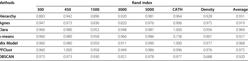
Table 2 Comparison of the clustering methods based on popular metrics

Methods Rand index

300 450 1500 3000 5000 CATH Density Average

Hierarchy 0.883 0.942 0.896 0.920 0.981 0.964 0.928 0.931

Agnes 0.947 0.973 0.836 0.820 0.976 0.906 0.975 0.919

Clara 0.960 0.980 0.952 0.948 0.987 1.000 0.956 0.969

k-means 0.960 0.980 0.958 0.966 0.986 0.738 0.901 0.927

Mix Model 0.960 0.980 0.959 0.911 0.990 1.000 0.977 0.968

PFClust 0.960 1.000 0.958 0.949 0.986 0.996 0.976 0.975

DBSCAN 0.973 0.973 0.930 0.921 0.978 0.977 0.688 0.920

We ran k-means and Clara 100 times each on every dataset and have selected as the final result for each algorithm the one with the best Silhouette width. For theepsilonparameter of DBSCAN, the maximum per-mitted distance between a point and its closest intra-cluster neighbour, we examined all values between 0 and 1

with a step size of 0.001. We also iterated themin-points

parameter, the minimum number of members allowed in

a valid cluster, using all integer values from 1 to 100. This

resulted in 105 clustering outputs, from which the one

with the maximum Silhouette width was selected.

As an addendum to the main work, we tested the use of the Silhouette width as a characteristic measure from which to decide the correct number of clusters. We ran the deter-ministic methods once each. We also ran the stochastic Clara and k-means algorithms 100 times each for every

A)Original B) Hierarchy C)Agnes

D)

E)k−means F)Mix Model G) PFClust H) DBSCAN

I) Original J) Hierarchy K) Agnes L) Clara

M) k−means N) Mix Model O) PFClust P) DBSCAN

number of clusters, k, between 2 and 50. The run with the best Silhouette width for a given algorithm was selected, thus deciding the number of clusters to report.

Protein fold clustering using polar Fourier expansions

A shape-density superposition algorithm based on Spher-ical Polar Fourier (SPF) basis functions has recently been

published [27,28], in which protein shapes are represented as 3D density functions expressed as expansions of ortho-normal basis functions:

ρðr;θ;φÞ ¼X N

nlm

αnlmRnlð Þr ylmðθ;φÞ

whereylm(θ,φ) are the real spherical harmonics,Nis the order of the highest polynomial power of the expansion,

Rnl(r) are radial functions, andαnlmare the expansion

co-efficients which are calculated as described previously [29].

Mavridis et al. proposed in the same paper a novel

structure-based indexing for existing classification schemes such as CATH [19] and SCOP [20]. Their proposed

consensus algorithm works well for only some of the cases it was tested on, because of the structural diversity of a number of protein domains assigned to the same super-families [28]. Hence, methods such as SPF would greatly benefit from an automated clustering algorithm, such as PFClust, which could identify the structure of a dataset without any prior knowledge or parameter tuning.

In order to illustrate that PFClust could be used to provide such a clustering using the SPF descriptors, we performed the following study. We randomly selected 11 CATH superfamilies, which had in total 224 non-redundant representative structures, and used the SPF descriptors to calculate the all-against-all similarity matrix of these protein domains. We then used PFClust

to cluster the protein domain structures based on these similarities.

Results and discussion

Original dataset

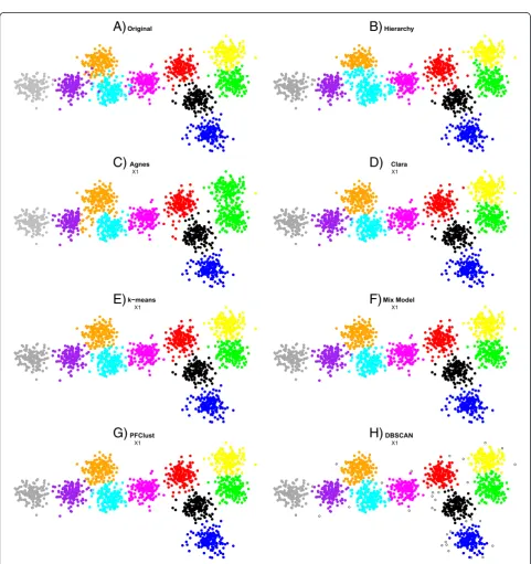
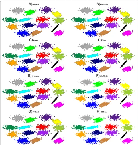
In this section, we present the resulting clusters from the 1500 2D vector dataset that was used for the general

parameter set up of the algorithm. Figure 3 shows the results of each method on the 1500 2D vector dataset; the mismatched points for each method are shown in Additional file 1: Figure S1. From the Rand Index re-sults in Table 2, we see that Agnes has the lowest (worst) score; that is mainly because Agnes joins two groups into a single cluster (green and yellow). Fur-thermore, we have a singleton as one cluster (yellow

point). Rather better levels of performance are

achieved by the Hierarchy and DBSCAN algorithms. However, Hierarchy has trouble in correctly assigning a number of the boundary cases for some pairs of clus-ters (particularly around the boundary between the or-ange and cyan clusters, and also that between yellow and green) and DBSCAN assigns a large number of points as singletons. Finally, the best performing algo-rithms are PFClust, Clara, k-means and Mix Model, which correctly identify all clusters and boundaries. Although the Rand Indices for these methods are very

good, they fail to reproduce perfectly the original‘

cor-rect’ classification because the original dataset has a

number of outlier points that lie closer to the centres of different groups, such as purple elements in the cyan and orange groups. So, for example, a purple element is so coloured because in the original grouping it was generated from the normal distribution used to define the purple cluster. However, it is located signifi-cantly closer to the centre of the cyan cluster, and thus we believe that a rational classifier should consider it cyan. Nonetheless, the gold standard we are using means that we count the rational classification as incorrect.

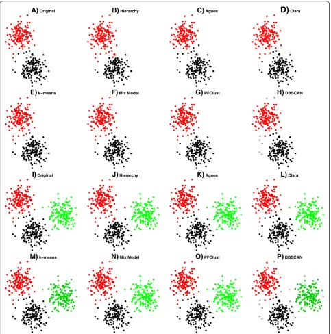
Validation

For the first two experiments with the 300 and 450 2D vectors, all methods perform very well, as shown in Figure 4, with only the Hierarchy clustering performing a little worse in comparison with the rest, as can be seen in Table 2 with the mismatched points for each method be-ing shown in Additional file 1: Figure S2.

Table 2 summarizes the results for all methods on all the different datasets used in this study. We can see from the results that PFClust is the top performing algo-rithm on average with a mean Rand Index of 0.975, though it perfectly reproduces the original clusters for only one dataset (450 2D vectors).

When we use all 3000 2D vectors, PFClust suggests a different number of clusters from that in the original clustering. In this case, PFClust finds that there are 21 clusters instead of 20 and splits the light green cluster into two, light green and gold. Even though PFClust sug-gests a different number of clusters, its very good Rand Index means that it still significantly outperforms the

other algorithms, except k-means, as can be seen in Table 2. Hierarchy, Clara and DBSCAN achieve good Rand Indices, though with some errors on the borderline cases. Mix Model gives a Rand Index that is only slightly worse, but assigns a singleton as one of its 20 clusters and, as seen in Figure 5, splits the greenish cluster at the top centre of the diagram between its purple and blue neighbours; the mismatched points for each method are shown in Additional file 1: Figure S3. DBSCAN identifies the correct number of multi-member clusters, although as with all datasets it additionally has a large number of points assigned as singletons, shown as open circles in Figure 5.

We also performed another validation study on the bigger dataset of 5000 2D vectors distributed over 15 clusters, in order also to compare the algorithms using a dataset that had different shapes and sizes of clusters, as well as the larger number of data points. As suggested by visual inspection of Figure 6, the Rand Index results in Table 2 show that all algorithms perform very well, with Mix Model having the best Rand Index. The mismatched points for each method are shown in Additional file 1: Figure S4.

Another challenge for algorithms is describing datasets that have different densities of points in their original clusters; the 928 2D vector dataset consists of 20 clusters whose densities vary. This is a subset of the D31 dataset taken from [30], which consists of 31 circular clusters with 100 members each. We then chose a 20 cluster subset of the original dataset and from each cluster we

Table 3 Supervised and Unsupervised timings for PFClust

Dataset Rand

index

Randomizations Clustering Total execution time (runs)

CATH folds

0.996 4.3 s 1.8 s 25 s

300 2D Vectors

0.960 8 s 2 s 40 s

450 2D Vectors

1.000 25 s 8 s 2 m 38 s

1500 2D Vectors

0.958 13 m 22 s 5 m 47s 1 h 22 m

3000 2D Vectors

0.949 2 h 24 m 27 s 1 h 14 m 38 s 12 h

5000 2D Vectors

0.986 11 h 35 m 30 s 5 h 20 m 20 s 81 h 50 m 30 s

Density Dataset

0.976 6 m 20 s 2 m 15 s 36 m

1500 Supervised

0.958 - 1 m 50 s 2 m 57 s

3000 Supervised

0.951 - 12 m 20 s 20 m 39 s

5000 Supervised

randomly selected a different number of members (vary-ing from 5% to 95%).

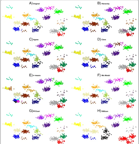
In this case, we see from Figure 7 that PFClust re-ports 19 clusters instead of the original 20, integrating the black group into the navy blue and the light green. Of the other methods, only Agnes was able to correctly identify all the groups, but due to the misassignment of some borderline cases it did not achieve a very high Rand Index. DBSCAN has major problems assigning the correct clusters (it finds only 10 multi-member ones), joining many clusters together and again leaving a

large number of singletons, as seen in Figure 7; the mismatched points for each method are shown in Additional file 1: Figure S5.

PFClust–supervised mode

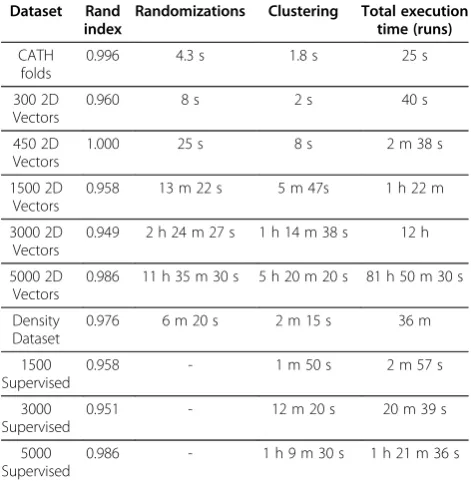
While we have shown PFClust to be a very powerful and accurate algorithm, it does take longer to cluster a dataset than most alternative approaches. Table 3 shows how the running time of the algorithm until convergence varies with the number of data points. It is easy to see that the run time grows rapidly as the dataset becomes larger and

Table 4 CATH superfamilies selected for the study

Superfamily Name Members Representative structure

1.20.140.10 Butyryl-CoA Dehydrogenase, subunit A, domain 3 13

1.25.40.20 - 21

2.80.10.50 - 40

2.30.42.10 - 55

2.40.100.10 Cyclophilin 10

2.40.110.10 Butyryl-CoA Dehydrogenase, subunit A, domain 2 7

3.30.500.10 Murine Class I Major Histocompatibility Complex, H2-DB, subunit A, domain 1 13

3.40.50.80 Nucleotide-binding domain of ferredoxin-NADP reductase (FNR) module 14

3.40.50.1220 TPP-binding domain 16

Table 4 CATH superfamilies selected for the study(Continued)

3.90.79.10 Nucleoside Triphosphate Pyrophosphohydrolase 24

The 11 CATH superfamilies that were selected to be clustered.

that the clustering takes considerable amounts of CPU time in order to converge, with most of it being spent in the randomization process.

The table summarizes the timings for convergence of PFClust with the different datasets. The total execution time typically includes four randomization and four clus-tering runs, but in the case of the 5000 2D vectors, the

“0.99 average Rand Index between the four clusterings”

criterion was not met until a fifth run had been carried

out. The second column in the table shows the Rand Index of the final clustering against the original gold standard cluster definitions.

There exist cases when one wants to cluster large groups of data and time efficiency is very important. For those cases, a supervised mode of PFClust has been implemented in order to significantly speed up the process. The super-vised mode of PFClust addresses the cost issue by applying an initial clustering on a training set and estimating a

V2 V3 V4 V5 V6 V7 V8 V9V10 V11 V12 V13 V14 V15 V16 V17 V18 V19 V20 V21 V22 V23 V24 V25 V26 V27 V28 V29 V30 V31 V32 V33 V34 V35 V36 V37 V38 V39 V40 V41 V42 V43 V44 V45 V46 V47 V48 V49 V50 V51 V52 V53 V54 V55 V56 V57 V58 V59 V60 V61 V62 V63 V64 V65 V66 V67 V68 V69 V70 V71 V72 V73 V74 V75 V76 V77 V78 V79 V80 V81 V82 V83 V84 V85 V86 V87 V88 V89 V90 V91 V92 V93 V94 V95 V96 V97 V98 V99V100 V101 V102 V103 V104 V105 V106 V107 V108 V109 V110 V111 V112 V113 V114 V115 V116 V117 V118 V119 V120 V121 V122 V123 V124 V125 V126 V127 V128 V129 V130 V131 V132 V133 V134 V135 V136 V137 V138 V139 V140 V141 V142 V143 V144 V145 V146 V147 V148 V149 V150 V151 V152 V153 V154 V155 V156 V157 V158 V159 V160 V161 V162 V163 V164 V165 V166 V167 V168 V169 V170 V171 V172 V173 V174 V175 V176 V177 V178 V179 V180 V181 V182 V183 V184 V185 V186 V187 V188 V189 V190 V191 V192 V193 V194 V195 V196 V197 V198 V199 V200 V201 V202 V203 V204 V205 V206 V207 V208 V209 V210 V211 V212 V213 V214 V215 V216 V217 V218 V219 V220 V221 V222 V223 V224 V225

DBSCAN PFClust Mix Model k−means Clara Agnes Hierarchy CATH

number of thresholds that would finally be applied to full dataset. The training set should be a small subset of the data, representing some coherent groups or clusters amongst the full dataset that we wish to cluster.

PFClust clusters the training set and uses the three best performing thresholds to estimate a total of nine threshold

values (these are selected to allow for some variation). Then these nine values are applied on the full dataset and the clustering with the best Silhouette width is reported. Using the supervised version of the algorithm the time-consuming randomization step is removed, which results in a significant speed-up of the total process.

0 10 20 30 40 50

0.0 0 .2 0.4 0 .6 0.8 1 .0 300 Members

Number of Clusters

Silhouette Width

0 10 20 30 40 50

0.0 0 .2 0.4 0 .6 0.8 1.0 450 Members

Number of Clusters

Silhouette Width

0 10 20 30 40 50

0.0 0.2 0 .4 0.6 0.8 1.0 1500 Members

Number of Clusters

Silhouette Width

0 10 20 30 40 50

0.0 0.2 0.4 0.6 0.8 1.0 3000 Members

Number of Clusters

Silhouette Width

0 10 20 30 40 50

0.0 0 .2 0.4 0.6 0.8 1 .0 5000 Members

Number of Clusters

Silhouette Width

0 10 20 30 40 50

0.0 0.2 0.4 0.6 0 .8 1.0 Density

Number of Clusters

Silhouette Width

5 10 15 20

0.0 0.2 0.4 0.6 0 .8 1.0 CATH

Number of Clusters

Silhouette Width Hierarchy Agnes Clara k−means Mix Model

As a validation of the supervised mode, we used the dataset with the 1500 vectors in 10 groups, the dataset of 3000 vectors distributed over 20 groups, and the lar-ger one of 5000 vectors distributed over 15 groups. Figure 8 shows the original dataset and the split between training and full sets, as well as the resulting classifica-tion by PFClust. A training set of 300 points was se-lected and PFClust running using the supervised mode clustered the first two datasets very rapidly, compared to the unsupervised version, and with high accuracy. In more detail, for the dataset of 1500 vectors the algo-rithm took only three minutes to complete and gave an identical clustering to the unsupervised method. For the 3000 vector group it took only 20 minutes, again with a very good Rand Index of 0.951 compared with the ori-ginal clustering, and in fact very slightly better than the 0.949 achieved by the unsupervised PFClust. Finally, for the larger group the algorithm used a training set of 626 vectors and took 1 hour and 21 minutes to complete, giving again a very good Rand Index of 0.986. In each case, the Rand Indices achieved by the supervised and unsupervised modes of PFClust are virtually identical, but the supervised mode is much faster.

Protein fold clustering using polar Fourier expansions

When we used PFClust to cluster the 224 protein domains in 11 CATH superfamilies, as shown in Table 4, the pro-gram reported 11 multi-member clusters and one single-ton protein domain, i.e., 12 clusters in total. Figure 9 shows as a heat map the all-against-all similarity matrix of protein domains, each row is colour coded according to the CATH classification and each column according to the PFClust clustering.

The agreement between PFClust and the CATH classification is nearly perfect with a Rand Index of 0.996. There is only a minor difference between the original classification and the classification of PFClust, where the 1q27A00 protein domain was classified as a singleton, whereas CATH has it assigned to the 3.90.79.10 superfamily. We also tested the other clus-tering algorithms against this dataset and set the num-ber of clusters to 11 for the five algorithms requiring this parameter. Table 2 summarizes the performance of each method, and Figure 10 visually shows the agreements and disagreements between the different clustering algo-rithms. We see that Mix Model and Clara are the top performing clustering algorithms, reproducing the exact CATH classification.

Finding the correct number of clusters

For each of the aforementioned datasets, we tested the use of the Silhouette width as the criterion for

identify-ing the number of clusters–similarly to the way we ran

DBSCAN. Since all the algorithms depended on a single

parameterk(number of clusters, inclusive of singletons),

we varied this number from 2 to 50 and the results are shown in Figure 11. Note that these data are consid-ered separately and do not contribute to the main re-sults described previously, for which purpose the

‘correct’ number of clusters was instead passed to

Hierarchy, Agnes, Clara, k-means and Mix Model as a parameter.

We see that in most cases, except for the density dataset, at least one method found the correct number of clusters by using the maximum Silhouette width as the stopping criterion. However, no method is consist-ently able to do this for the different datasets.

Conclusions

It has been shown that PFClust can accurately group data according to their similarities without the need for any parameter tuning. Our clustering results on the synthetic datasets not only show that PFClust provides structurally meaningful clusters, but also that it performs best when compared to six other well-known clustering algorithms. Clustering protein domains using a density representation gives excellent agreement with the CATH part-manually curated classification. In the future, the full CATH data-base could be automatically clustered data-based on such dens-ity representations of protein domains.

Additional file

Additional file 1: Figure S1.Comparison of different clustering algorithms;Figure S2.Comparison of the 300 and 450 2D vector datasets;Figure S3.Comparison of different clustering algorithms;

Figure S4.Comparison of different clustering algorithms;Figure S5.

Comparison of different clustering algorithms;Table S1.R packages used in the comparison of different clustering methodologies.

Competing interests

The authors have received funding from WADA. Other than this sponsorship, the authors declare no conflict of interest.

Authors_’contributions

LM conceived and implemented the algorithm, carried out the experiments with PFClust and participated in the drafting of the manuscript. LM and NN designed the experimental and validation studies and carried out the comparison of PFClust with the other methods. NN participated in the drafting of the manuscript. JBOM participated in the drafting of the manuscript and provided guidance. All authors read and approved the final manuscript.

Acknowledgements

This project has been carried out with the support of WADA. JBOM and NN thank the Scottish Universities Life Sciences Alliance (SULSA) and the Scottish Overseas Research Student Awards Scheme of the Scottish Funding Council (SFC) for financial support. We thank Dr Luna De Ferrari for her valuable comments on this manuscript.

Availability

By request to the corresponding author, [email protected].

References

1. Harlow TJ, Gogarten JP, Ragan MA:A hybrid clustering approach to recognition of protein families in 114 microbial genomes.BMC Bioinformatics2004,5:45.

2. Zhu X:Semi-Supervised Learning Literature Survey.Technical Report 1530, Department of Computer Sciences.Madison: University of Wisconsin; 2005. http://pages.cs.wisc.edu/~jerryzhu/pub/ssl_survey.pdf.

3. Pise NN, Kulkarni P:A Survey of Semi-Supervised Learning Methods. International Conference on Computational Intelligence and Security2008, 30:34 [http://ieeexplore.ieee.org/stamp/stamp.jsp?tp=&arnumber=4724730]. 4. Jain A, Murty M, Flynn P:Data clustering: a review.ACM Comput Surv1991,

31:264–323.

5. Handl J, Knowles J, Kell DB:Computational cluster validation in post-genomic data analysis.Bioinformatics2005,21:3201_–3212. 6. Lance BGN, Williams WT:A general theory of classificatory sorting

strategies 1. Hierarchical systems.Comput J1967,9:373–380. 7. Jain AK:Data clustering: 50 years beyond K-means.Pattern Recognition

Letters2010,31:651–666.

8. Tibshirani R, Walther G, Hastie T:Estimating the number of clusters in a data set via the gap statistic.Journal of the Royal Statistical Society Series B Statistical Methodology2001,63:411–423.

9. Giancarlo R, Scaturro D, Utro F:Computational cluster validation for microarray data analysis: experimental assessment of Clest, Consensus Clustering, Figure of Merit. Gap Statistics and Model Explorer.BMC Bioinformatics2008,9:462.

10. Rousseeuw P:Silhouettes: a graphical aid to the interpretation and validation of cluster analysis.J Comput Appl Math1987,20:53–65. 11. Dunn JC:A Fuzzy Relative of the ISODATA Process and Its Use in

Detecting Compact Well-Separated Clusters.J Cybernetics1973,3:32–57. 12. Bezdek JC, Pal NR:Some new indexes of cluster validity.IEEE transactions

on systems, man, and cybernetics. Part B, Cybernetics1998,28:15. 13. Rand WM:Objective Criteria for the Evaluation of Clustering Methods.

J Am Stat Assoc1971,66:846–850.

14. Akoglu L, Tong H, Meeder B, Faloutsos C:PICS: Parameter-free Identification of Cohesive Subgroups in Large Attributed Graphs.Anaheim, CA: SDM; 2012. 15. Shenoy SR, Jayaram B:Proteins: sequence to structure and function–

current status.Curr Protein Pept Sci2010,11:498_–514.

16. Wu CH, Huang H, Arminski L, Castro-Alvear J, Chen Y, Hu ZZ, Ledley RS, Lewis KC, Mewes HW, Orcutt BC, Suzek BE, Tsugita A, Vinayaka CR, Yeh LSL, Zhang J, Barker WC:The Protein Information Resource: an integrated public resource of functional annotation of proteins.Nucleic Acids Res 2002,30:35–37.

17. Finn RD, Mistry J, Tate J, Coggill P, Heger A, Pollington JE, Gavin OL, Gunasekaran P, Ceric G, Forslund K, Holm L, Sonnhammer ELL, Eddy SR, Bateman A:The Pfam protein families database.Nucleic Acids Res2010, 38:D211–D222.

18. Berman HM, Westbrook J, Feng Z, Gilliland G, Bhat TN, Weissig H, Shindyalov IN, Bourne PE:The Protein Data Bank.Nucleic Acids Res2000, 28:235_–242.

19. Cuff AL, Sillitoe I, Lewis T, Redfern OC, Garratt R, Thornton J, Orengo CA: The CATH classification revisited–architectures reviewed and new ways to characterize structural divergence in superfamilies.Nucleic Acids Res 2009,37:D310–314.

20. Murzin AG, Brenner SE, Hubbard T, Chothia C:SCOP: a structural classification of proteins database for the investigation of sequences and structures.J Mol Biol1995,247:536–540.

21. Berman HM:The Protein Data Bank: a historical perspective.Acta Crystallographica Section A Foundations of Crystallography2008,64:88–95. 22. Kaufman L, Rousseeuw PJ:Finding Groups in Data: An Introduction to Cluster

Analysis.New York: Wiley; 1990.

23. Wei C:Empirical Comparison of Fast Clustering Algorithms for Large Data Sets.Experts Systems with Applications2003,24:351–363. 24. Ester M, Kriegel HP, Sander J, Xu X:A Density-Based Algorithm for

Discovering Clusters in Large Spatial Databases with Noise. Proceedings of 2nd International Conference on Knowledge Discovery and Data Mining. 1996:226–231. KDD-96.

25. Fraley C, Raftery AE:Model-based clustering, discriminant analysis, and density estimation.J Am Stat Assoc2002,97:611_–631.

26. R: A language and environment for statistical computing; R development core team.Vienna, Austria: R foundation for statistical computing; 2005. http:// www.r-project.org/.

27. Mavridis L, Ritchie DW:3D-Blast: 3D protein structure alignment, comparison, and classification using spherical polar fourier correlations. Pac Symp Biocomput2010:281–292.

28. Mavridis L, Ghoorah AW, Venkatraman V, Ritchie DW:Representing and comparing protein folds and fold families using three-dimensional shape-density representations.Proteins: Structure, Function and Bioinformatics2011,80:530–545.

29. Ritchie DW, Kemp GJ:Protein docking using spherical polar Fourier correlations.Proteins2000,39:178–194.

30. Veenman CJ, Reinders MJT, Backer E:A maximum variance cluster algorithm.Pattern Analysis and Machine Intelligence, IEEE Transactions2002, 24:1273–1280.

doi:10.1186/1471-2105-14-213

Cite this article as:Mavridiset al.:PFClust: a novel parameter free clustering algorithm.BMC Bioinformatics201314:213.

Submit your next manuscript to BioMed Central and take full advantage of:

• Convenient online submission

• Thorough peer review

• No space constraints or color figure charges

• Immediate publication on acceptance

• Inclusion in PubMed, CAS, Scopus and Google Scholar

• Research which is freely available for redistribution