Generalizing MOND to explain the missing mass in galaxy clusters

December 19, 2016

Generalizing MOND to explain the missing mass in galaxy clusters

Alistair O. Hodson

and Hongsheng Zhao

1_{SUPA, School of Physics and Astronomy, University of St Andrews, Scotland}

e-mail:[email protected]

Received , ; accepted ,

ABSTRACT

Context.Modified Newtonian Dynamics (MOND) is a gravitational framework designed to explain the astronomical observations in the Universe without the inclusion of particle dark matter. Modified Newtonian Dynamics, in its current form, cannot explain the missing mass in galaxy clusters without the inclusion of some extra mass, be it in the form of neutrinos or non-luminous baryonic matter. We investigate whether the MOND framework can be generalized to account for the missing mass in galaxy clusters by boosting gravity in high gravitational potential regions. We examine and review Extended MOND (EMOND), which was designed to increase the MOND scale acceleration in high potential regions, thereby boosting the gravity in clusters.

Aims.We seek to investigate galaxy cluster mass profiles in the context of MOND with the primary aim at explaining the missing mass problem fully without the need for dark matter.

Methods.Using the assumption that the clusters are in hydrostatic equilibrium, we can compute the dynamical mass of each cluster and compare the result to the predicted mass of the EMOND formalism.

Results.We find that EMOND has some success in fitting some clusters, but overall has issues when trying to explain the mass deficit fully. We also investigate an empirical relation to solve the cluster problem, which is found by analysing the cluster data and is based on the MOND paradigm. We discuss the limitations in the text.

Key words. Gravitation – – Galaxies: clusters:general

1. Introduction

To explain dynamics in astrophysical system fully, a solution to the missing mass problem that plagues astrophysics to this day must be imposed. Commonly, the missing mass in our Universe is explained away by the existence of some non-baryonic dark matter. Although dark matter is thought by most to be the best solution to the missing mass problem, despite our best efforts to date, the lack of direct detection has led some to explore other ex-planations. To do this, it is possible to think of Newtonian gravity as a limit of a more general gravity law. An example of a modi-fied theory of gravity, designed with the absence of dark matter in mind, is Modified Newtonian Dynamics, hereafter MOND. The MOND paradigm works with the principle that Newtonian gravity breaks down in the low acceleration limit (a<<a0where a0is an acceleration constant≈1.2×10−10ms−2).

Originally, MOND was proposed and introduced as an em-pirical law in the 1983 Milgrom 1983 papers (Milgrom 1983a), (Milgrom 1983b) and (Milgrom 1983c) by analysing galaxy ro-tation curves. One issue with the original MOND formulation by Milgrom, which was highlighted in Felten (1983), was its inabil-ity to conserve momentum. This was rectified in the Bekenstein and Milgrom paper (Bekenstein & Milgrom 1984) by introduc-ing a Lagrangian formulation of MOND, AQUAL (A QUAdratic Lagrangian). Recently, Milgrom proposed an alternative formu-lation to the MOND paradigm called Quasi-Linear MOND (Mil-grom 2010), hereafter QUMOND. This new formulation is much more desirable as the quasi-linear way in which the MOND grav-ity is calculated is much simpler than in AQUAL.

The MOND framework has enjoyed a vast amount of suc-cess, providing reasonable descriptions of the dynamics in galax-ies. Arguably the most famous prediction of MOND is that of the

baryonic Tully-Fisher relation, which shows a correlation with total enclosed baryonic mass and galactic outer rotation veloc-ity (the flat part of the rotation curve) (McGaugh 2005). This correlation is explained naturally in the MOND paradigm. Also, MOND is very successful in predicting galaxy rotation curve profiles; see for example Sanders & McGaugh (2002). A further prediction of MOND was the nature of dwarf galaxies. MOND predicts that in the low acceleration regime there should be a high mass deficit (Milgrom 1983c). In other words, MOND pdicts that if objects are low surface brightness, they should re-quire a lot of dark matter, which is exactly what is found in dwarf galaxies. Tidal dwarf galaxies (TDGs) are also hard to explain in theΛCDM paradigm as their formation process does not predict the dragging of large amounts of dark matter away from their host galaxy (see for example Section 6.5.4 of Famaey & Mc-Gaugh (2012) and references therein). The formation of TDGs is more easily explained in MOND (Combes & Tiret 2010). For a more detailed review of the successes of MOND, we refer the reader to Famaey & McGaugh (2012).

Despite the success of MOND with regards to galaxy dynam-ics, MOND is not without its issues. Firstly, to be a viable gravity theory there must be a relativistic formulation, analogous to Ein-stein’s general relativity. There have been a few proposed rela-tivistic theories that produce MOND as a non-relarela-tivistic limit including, for example, Tensor-Vector-Scalar gravity (TeVeS) (Bekenstein 2004), the Dark Fluid model (Zhao 2007) and Bi-metric MOND (Milgrom 2009). However, these have their limi-tations and do not rival the success of general relativity.

Another major problem for MOND, and the topic of this paper, is the limited success when trying to describe the mass deficit in clusters of galaxies; see for example Sanders (1999) and Sanders (2003). It has been well documented that the

ferred mass by MOND in galaxy clusters is not enough to keep the cluster in hydrostatic equilibrium. This result is enough for some to abandon MOND as a viable theory. It is therefore the responsibility of those who study MOND to provide a suitable explanation as to why this missing mass problem arises. The suc-cessful predictions that were made using MOND have led some to believe that the inability to reproduce the galaxy cluster data is just a prediction that there exists some additional mass compo-nent that we are yet to detect. One possibility is that MOND and dark matter of some kind are not mutually exclusive and there exist both a breakdown of Newtonian dynamics in the small ac-celeration regime and some kind of elusive particle, increasing the available mass budget in clusters. This matter could be in the form of 2 eV neutrinos, which was suggested in Sanders (2003). However, analysis of a sample of galaxy clusters by Angus et al. (2008) found that the 2 eV neutrino was able to explain the mass deficit in the outer regions of the cluster with missing mass still remaining in the central regions. This would warrant the exis-tence of a different type of neutrino. An 11 eV sterile neutrino was investigated by Angus (2009), which was found to be suf-ficient to explain the galaxy cluster issue. Further investigation into solving galaxy clusters in MOND with the aid of neutri-nos was conducted in Angus & Diaferio (2011) and Angus et al. (2013). Cosmological simulations showed that it was possible to form clusters using hot dark matter (sterile neutrinos). How-ever, the results showed an underabundance of low mass clusters (attributed to the resolution of the simulation) and an overabun-dance of high mass clusters. They go on to explain how the 11 eV neutrino was ruled out as a neutrino mass of 30-300 eV was required to produce enough low mass clusters.

Neutrinos have not been the only attempt to reconcile clus-ters with MOND. Zhao and Li investigated a family of gravity models controlled by a vector field (see for example Li & Zhao (2009) and Zhao & Li (2010). This family of solutions can re-produce different types of behaviour depending on the model parameter choices. This is based on the assumption that there exists some dark fluid, described by the vector field, which is the source of deviation from Newtonian physics. Another attempt to solve the cluster problem proposed by Khoury (2015) also pos-tulates there exists a dark fluid that permeates space. This idea is motivated by the success of MOND on the galactic scale, but the success ofΛCDM in cosmological and cluster scales. This dark fluid formalism aims to recover galaxy scale dynamics via a MOND-like phonon mediated force resulting from the dark mat-ter in its superfluid phase. Clusmat-ters, in this scenario, would be dominated by the normal phase of the superfluid, which would behave like particle dark matter. This aims for a best of both worlds scenario with regards to dark matter and MOND. There has also been a theory proposed by Blanchet (2007), which in-cludes a substance called dipolar dark matter. This mechanism works on the principle that we do not actually see a breakdown of a gravity law when we empirically see MOND, but what we are witnessing is an enhancement of gravity due to dipole mo-ments of this exotic dark matter aligning with the gravitational field. All these theories have pros and cons, but are not studied in this work.

Although the aforementioned solutions may hold the keys to the cluster success in MOND, the need for dark matter of any kind has left some unsettled, as the elegance of MOND, in galax-ies, is the ability to account for all observations from visible mat-ter only. Therefore aside from these dark fluid-like theories, it has also been noted that if the value ofa0were to be increased in clusters, the mass discrepancy could be alleviated. In the same manner that MOND is a more general form of Newtonian

dy-namics, perhaps MOND in its current form is not universal, but part of a larger gravitational law. The generalization of MOND should not be ruled out hastily given the inherently empirical na-ture of its formulation. MOND was devised by studying rotation curves, as information of galaxy clusters was limited. Any new adaptation of MOND that increasesa0in clusters would have to somehow shield galaxies, where MOND works well, from the effects of this varying acceleration scale. This idea was formally outlined by Zhao & Famaey (2012) in the form of Extended Modified Newtonian Dynamics or EMOND.

Another issue in MOND is the newly discovered ultra diffuse galaxies (UDGs) (Mihos et al. 2015), (Koda et al. 2015). Ultra-diffuse galaxies are extremely low density galaxies, residing in the potential wells of galaxy clusters, which require a lot of dark matter. This required dark matter could be explained in MOND if it were not for the high external field exhibited on the UDGs by the galaxy cluster. The external field of the cluster raises the acceleration in the UDG, making the MOND prediction closer to Newtonian. This could be counteracted if the value ofa0were in fact larger in these environments as deviations from Newtonian gravity could occur at higher accelerations. The fact that a higher value ofa0 in galaxy clusters could simultaneously explain the mass deficit problem and the observations of these UDGs is in-teresting and should thus be explored in more detail.

This paper is outlined as follows. Section 2 outlines the MOND formalism and briefly reviews the missing mass prob-lem in clusters with MOND. This is followed by a review of the EMOND formalism. Section 3 discuses the galaxy cluster sample that we have used throughout the paper. Section 4 dis-cusses how well EMOND works in explaining the missing mass problem. We find that EMOND has partial success in tackling this problem and thus in Section 5 we try to find an empirical relation, based on the MOND paradigm, which can account for the cluster mass deficit. We find a potential relation, with some success as well, which we compare to the Navarro-Frenk-White (hereafer NFW) fits described in (Vikhlinin et al. 2006) in Sec-tion 6. In SecSec-tion 7 we discuss the limitaSec-tions of this empirical relation and we conclude in Section 8.

2. Summarizing the MOND-cluster problem

2.1. The MOND paradigm and its limitations

We begin by briefly reviewing the MOND paradigm and its gov-erning equations. The general motivation for MOND the recog-nition that the Newtonian prediction of gravity only seemed to fail in low acceleration environments. If there is no non-baryonic dark matter to explain this discrepancy, the gravitational law governing the Universe would have to deviate from Newtonian in these low acceleration environments.

In Newtonian physics, the gravitational fieldΦis determined from the matter distributionρvia Poisson’s equation,

∇2Φ =4πGρ. (1)

Determining the gravitational field predicted by MOND re-quires an alternate Poisson equation (Bekenstein & Milgrom 1984),

∇ ·

"

µ |∇Φ|

a0 !

∇Φ

#

=4πGρ, (2)

µ(x)= (

1 forx1

x forx1. (3)

The first case of Equation 3 is the Newtonian regime and the second is known as the deep-MOND regime. The Newtonian Poisson equation is recovered in the x >> 1 case of Equation 3. One should note here that the centres of galaxy clusters have strong gravity, meaning they have anx>1 MOND value.

There are many possible functional forms forµ(x) that sat-isfy the criteria of Equation 3. We opted to choose the simple interpolation function (Famaey & Binney 2005),

µ(x)= x

1+x, (4)

for our analysis.

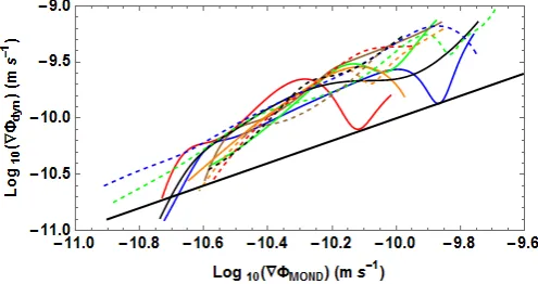
The MOND paradigm has always struggled with rectifying the mass discrepancy in galaxy clusters without including an ex-tra mass component such as neutrinos or non-luminous baryonic matter. In its usual form MOND is unable to boost the grav-itational acceleration in clusters sufficiently whilst this frame-work is still able to match observational constraints provided by galaxy dynamics. The reason for MOND’s inability to accom-plish this is that the gravitational acceleration in galaxy clusters is relatively high, in general x>1, so the MOND boost to gravity is weak. However, there is an observed mass deficit in galaxy clusters that would require the cluster to be in the deep-MOND regime (x<<1) to rectify with MOND alone. We demonstrate this issue briefly by applying MOND to the cluster sample de-scribed in Section 3. We can plot the dynamical acceleration (See Section 3 for details on how the dynamical acceleration is cal-culated) for each cluster against the corresponding MOND com-puted acceleration from Equation 2; see (Figure 1). If MOND were a universal law that applied to galaxy clusters, Fig 1 should show 1:1 correlation (within observational errors), by which we mean that the gravitational acceleration predicted by the MOND formula should match the gravitational acceleration predicted by the dynamics of the X-ray gas. In Figure 1, we see that the re-quired gravitational acceleration, derived from the dynamics of the X-ray gas, exceeds the gravitational acceleration predicted by the MOND formula. Thus MOND is under-predicting the gravitational acceleration of each cluster. As mentioned previ-ously, this offset is often reconciled in the MOND paradigm by the presence of some form of non-luminous baryonic matter or neutrinos, which has yet to be detected.

2.2. Can MOND be generalized to account for clusters?

As the simple MOND formulation does not hold true for galaxy clusters, efforts were made to try and generalize MOND. In order to do this, one must identify what, if any, are the critical diff er-ences between galaxies and galaxy clusters. One such difference is that the gravitational potential is much larger in galaxy clus-ters than in galaxies. In its current form, MOND has a functional dependence solely on gravitational acceleration. Perhaps a more universal gravity law requires gravitational potential as a media-tor of total gravity. Again, using the cluster sample described in Section 3, we can see how the gravitational acceleration of the cluster varies as a function of gravitational potential (see Figure 2). In Figure 2, we made the approximation that the gravitational potential of the cluster is equal to the contribution of the dark matter, described by a NFW profile (Navarro et al. 1997), (Zhao

Fig. 1.Plot showing how the dynamical (or total) gravitational acceler-ation of the cluster compares to the gravitacceler-ational acceleracceler-ation predicted by MOND with a 1:1 line overplotted for illustrative purposes. Each line is a different cluster. We use 12 clusters from Vikhlinin et al. (2006). As the clusters lie above the 1:1 line (black solid line on plot), the required gravity is more than the ‘MOND predicted’ gravity.

12.0 12.2 12.4 12.6 12.8 13.0 0

1.×10-10 2.×10-10 3.×10-10 4.×10-10 5.×10-10 6.×10-10

Log10(|ΦNFW|) (m2s-2₎ aDyn

(

ms

-2)

Fig. 2.Plot showing how the dynamical gravitational acceleration varies with NFW potential for each cluster in our sample. NFW profiles were taken from Vikhlinin et al. (2006). Note the regular trend between the clusters, which suggests a modified gravity law dependent on gravita-tional potential.

1996). The NFW profile for each cluster was given in Vikhlinin et al. (2006). We made this approximation as the dark matter NFW profile is analytical and well defined, whereas computing the gravitational potential from the dynamical data requires us to know where the edge of the cluster lies in order to truncate the mass. Furthermore, we would have to perform an unneces-sary additional step of numerically integrating the dynamical ac-celeration to find the potential. This integration would involve a boundary value that is dependent on the truncation radius of the cluster. As we are only interested in getting an intuition of how the properties of the galaxy clusters correlate with gravita-tional potential, the NFW approximation seems to be reasonable compared to performing the integration of the dynamical accel-eration.

This trend with potential was the main motivation of the Zhao and Famaey Extended MOND (EMOND) formalism (Zhao & Famaey 2012). In EMOND, the corresponding Poisson equation is written as

4πGρ=∇ ·

"

µ |∇Φ|

A0(Φ) !

∇Φ

#

−T2, (5)

where

T2= 1 8πG

d(A0(Φ))2 dΦ

_yF0_(y)−F(y), ₍₆₎

whereA0(Φ) is a functional alternative to the MOND constant a0with units of acceleration, andµis the same MOND interpo-lation function,dF(y)/dy=µ(√y) andy =|∇Φ|2_/A

0(Φ)2. It is immediately apparent that Equation 5 is much more complicated than the regular MOND Poisson equation owing to the second term. It has however been argued that in certain situations, such as galaxy clusters, this term is small compared to the first (Zhao & Famaey 2012), giving an approximate expression,

4πGρ≈ ∇ ·

"

µ |∇Φ|

A0(Φ) !

∇Φ

#

, (7)

for the EMOND gravitational potential. In Section 4 we explic-itly show that we are just in making this approximation. Equation 7, the approximate EMOND Poisson equation, is equivalent to Equation 2 with a modified scale acceleration. The idea behind Equation 7 is to increase the MOND acceleration scale in high potential environments. This decreases the value of the MOND interpolation function,µ, thus increasing the total gravitational acceleration that is predicted by MOND (aMOND ≈aNewt/µ). In

order to solve the EMOND Poisson equation, we must define the behaviour ofA0(Φ), which we discuss in Section 4. Although we determine the exact behaviour ofA0in Section 4, we should pro-vide some understanding of the general desired behaviour that we hope to emulate. From our understanding of galaxy rotation curves in MOND, we know that in general galaxies are well de-scribed by a constanta0 ≈1.2×10−10ms−2. We therefore want to preserve this behaviour. Therefore the standarda0should be a limit ofA0in the low potential regime such thatA0(Φ)→a0 as Φ→0.

2.3. The external potential effect

As the modification to the MOND formula we discuss here re-lies on the gravitational potential, even a constant gravitational potential across a system from an external source affects the dy-namics. This feature can be thought of as an external potential effect (Zhao & Famaey 2012), which is analogous to the ex-ternal field effect (EFE) that arises in regular MOND; see for example Derakhshani & Haghi (2014) for work on the EFE in globular clusters; Blanchet & Novak (2011), which looks at the EFE in the solar system; and Haghi et al. (2016), for work with the EFE and declining rotation curves in MOND. The treatment of the external potential effect should be fully examined in fu-ture work. The original EMOND work assumes that the main contribution to the external potential of the Milky Way can be attributed to the Virgo cluster. Work on the escape velocity of the Milky Way (Famaey et al. 2007) calculates the external potential for the Milky Way to be approximatelyΦext ≈ −10−6c2.

How-ever, the typical gravitational potentials of our galaxy clusters are much larger than this so we are able to exclude this effect from our calculations. The importance of the external potential effect is most prominent in galaxies and objects that lie within clusters or near objects with large gravitational potentials. For example, we mentioned earlier that there has recently been a discovery of many so-called ultra diffuse galaxies (UDGs) inside galaxy clusters. The existence of these objects could pose some threat to MOND as the external field from the clusters should make the dynamics inside UDGs closer to Newtonian (µ(x) → 1). However, if this external potential effect was present, the fact that the UDGs are within the deep potential well of the galaxy clusters could cause UDGs to show MOND-like behaviour or at least exhibit stronger gravity than that expected from Newtonian

physics. The external potential effect could be a natural explana-tion as to why objects exist within clusters that behave similar to UDGs. However, recent estimates of dark matter haloes in these objects show an extremely high dark to baryonic mass ratio (van Dokkum et al. 2016). One would need to check that the exter-nal potential effect required to reconcile that the UDGs does not conflict with the host galaxy cluster.

3. Analysing a galaxy cluster sample

To begin, we first need to select a galaxy cluster sample. We use a Chandra galaxy cluster sample (Vikhlinin et al. 2006) that provides analytical fits to the temperature and density profiles of the X-ray gas. We use 12 clusters from the sample. The clusters are nearby (z<1) and are in the mass range≈1014₋₁₀15_M

. For a thorough analysis, we also need to model the brightest cluster galaxy (BCG) component. The BCG modelling is outlined in Section 3.1.1.

3.1. Cluster model

To model the X-ray gas density Vikhlinin et al. (2006) chooses an analytical expression to which the data is fit. This model is composed of three parts. The first part models the cuspy core usually found in relaxed clusters and is achieved by a power law density profile. They then include an additional term that models the steepening brightness profile atr>0.3r200, wherer200is the radius at which the average density of the cluster falls to 200 times that of the critical density of the Universe. They finally add another power law component to allow the density profile to be very general for fitting freedom. Combining these three components leads to their overall emission profile for the X-ray gas,

nenp(r)=n20

(r/rc)−α

1+(r/rc)2

3β−α/2

1

(1+(r/rs)γ)/γ

+ n

2 0

1+(r/rc2)2 3β2. (8)

whererc,rc2, andrsare all scale radii andα,β,γ,, andβ2are all dimensionless parameters.neandnpare electron and proton

number densities, andn0is a parameter that takes the meaning of a central number density. The emission profile is converted into

the mass density byρg(r)≈1.252mp

npne

1/2

, wherempis the

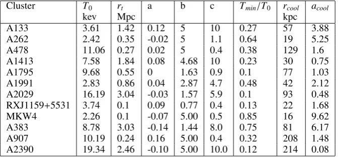
mass of a proton. The parameter fits for each galaxy cluster are given in Table 1, which were taken from Vikhlinin et al. (2006). We also require the temperature profile of the gas as we are choosing to relax the common assumption that the galaxy clus-ters are isothermal. Again, we follow the profile provided by Vikhlinin et al. (2006),

T(r)=T0

(r/rcool+Tmin/T0) (r/rcool)acool+1

(r/rt)−a

(r/rt)b+1

c/b, (9)

which accounts for the cooling of the X-ray gas in the central regions of the cluster, which according to Vikhlinin et al. (2006) may be the result of radiative cooling. The parameterTminis the

central temperature, T0 is a scale temperature, rcool andrt are

scale radii, andacool, a b and c are dimensionless parameters.

Table 1.Table of parameters as given in Vikhlinin et al. (2006) for the X-ray gas emission profile described by Equation 8. We omitted one cluster from our analysis as Vikhlinin et al. (2006) do not provide NFW fits for dark matter, so we cannot compare our result to that in a consistent manner.γfor each cluster was chosen to be 3.0. Values in table labelled N/A refer to the clusters for which (Vikhlinin et al. 2006) did not provide parameters, making those clusters a two-component density model rather than three (see Equation 8).

Cluster n0 rc rs α β n02 rc2 β2

(10−3cm−3) (kpc) (kpc) (10−1cm−3) (kpc)

A133 4.705 94.6 1239.9 0.916 0.526 4.943 0.247 75.83 3.607

A262 2.278 70.7 365.6 1.712 0.345 1.760 N/A N/A N/A

A478 10.170 155.5 2928.9 1.254 0.704 5.000 0.762 23.84 1.00

A1413 5.239 195.0 2153.7 1.247 0.661 5.000 N/A N/A N/A

A1795 31.175 38.2 682.5 0.195 0.491 2.606 5.695 3.00 1.00

A1991 6.405 59.9 1064.7 1.735 0.515 5.000 0.007 5.00 0.517

A2029 15.721 84.2 908.9 1.164 0.545 1.669 3.510 5.00 1.00

RXJ1159+5531 0.191 591.9 640.7 1.891 0.838 4.869 0.457 11.99 1 .00

MKW4 0.196 578.5 595.1 1.895 1.119 1.602 0.108 30.11 1.971

A383 7.226 112.1 408.7 2.013 0.577 0.767 0.002 11.54 1.00

A907 6.252 136.9 1887.1 1.556 0.594 4.998 N/A N/A N/A

A2390 3.605 308.2 1200.0 1.891 0.658 0.563 N/A N/A N/A

Table 2.Table of gas temperature parameters as given in (Vikhlinin et al. 2006) for Equation 9.

Cluster T0 rt a b c Tmin/T0 rcool acool

kev Mpc kpc

A133 3.61 1.42 0.12 5 10 0.27 57 3.88

A262 2.42 0.35 -0.02 5 1.1 0.64 19 5.25

A478 11.06 0.27 0.02 5 0.4 0.38 129 1.6

A1413 7.58 1.84 0.08 4.68 10 0.23 30 0.75

A1795 9.68 0.55 0 1.63 0.9 0.1 77 1.03

A1991 2.83 0.86 0.04 2.87 4.7 0.48 42 2.12

A2029 16.19 3.04 -0.03 1.57 5.9 0.1 93 0.48

RXJ1159+5531 3.74 0.1 0.09 0.77 0.4 0.13 22 1.68

MKW4 2.26 0.1 -0.07 5.00 0.5 0.85 16 9.62

A383 8.78 3.03 -0.14 1.44 8.0 0.75 81 6.17

A907 10.19 0.24 0.16 5.00 0.4 0.32 208 1.48

A2390 19.34 2.46 -0.10 5.00 10.0 0.12 214 0.08

3.1.1. BCG model

We also model the brightest cluster galaxy (BCG) for each clus-ter, which affects the central parts of the cluster. This is an im-portant aspect of the model as it is in the central regions of the clusters where the mass deficit is greatest. To model the BCG, it is reasonable to make the approximation that it is spherical, with a density following the well-known Hernquist profile,

ρBCG(r)=

Mh

2πr(r+h)3, (10)

where M is the BCG mass and h is the BCG scale length. We assign a BCG mass proportional to the overall mass of the

clus-ter such thatMBCG=5.3×1011

M500

3×1014_M

0.42

M, which follows the work of Schmidt & Allen (2007). Here,M500is the enclosed mass at r500, which is the radius at which the average density is 500 times the critical density of the Universe. We also assign each cluster a Hernquist scale length of 30 kpc. Although these estimates may be crude, the BCG should only affect the inner parts of the cluster and thus should not affect our overall conclu-sions too much.

3.1.2. Radial range of the data

The radial range of the X-ray data is limited by two factors: an inner boundary or cut-off radius and an upper bound

ra-dius where the X-ray brightness is not detected. Vikhlinin et al. (2006) choose an inner radial boundary such that they exclude the central temperature bin and an outer radial boundary where the X-ray brightness is no longer detected above 3σor the limit of the Chandra field of view was reached. Therefore the model is fit to a section of the radial extent of the cluster, between these two limits, and then extrapolated to lower and higher radii. In Table 3, we show the inner most radii as given in Vikhlinin et al. (2006). For our plots throughout this paper, we choose not to show any data below this radius.

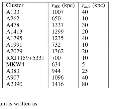
For the outer radius we choose to extrapolate past the maxi-mum radius of each cluster. We extrapolate to the radiusr200for each cluster, which can be crudely calculated viar200 ≈1.5r500 (Vikhlinin et al. 2006). The r500 values from Vikhlinin et al. (2006) are also shown in Table 3.

3.2. Dynamical mass of the clusters

In the following sections we show the results of dynamical masses, potentials, and accelerations so we therefore must de-fine these quantities. When we discuss ‘dynamical’ quantities in this work, we refer to the value calculated by assuming the clus-ter gas is in hydrostatic equilibrium. This is a common assump-tion in determining cluster masses. The equaassump-tion for hydrostatic

Table 3.r500values for each cluster as given in (Vikhlinin et al. 2006); r200values can be calculated approximately viar200≈1.5r500.

Cluster r500(kpc) rmin(kpc)

A133 1007 40

A262 650 10

A478 1337 30

A1413 1299 20

A1795 1235 40

A1991 732 10

A2029 1362 20

RXJ1159+5331 700 10

MKW4 634 5

A383 944 25

A907 1096 40

A2390 1416 80

equilibrium is written as

dΦdyn dr =

GMdyn(r) r2 =−

1

ρg(r) d dr

"ρ

gkT(r) wmp

#

, (11)

whereΦdyn is the dynamical potential,mp is the mass of a

pro-ton (≈ 1.67×10−27 _{kg), andwis the mean molecular weight} (≈0.609). The valueρg(r) is the gas density,T(r) is the gas

tem-perature, and Mdyn(r) is the enclosed dynamical mass at radius

r. Using some mathematical prowess, Equation 11 can be trans-formed into

Mdyn(r)=− kT(r)r Gwmp

"_dlnρ

g(r) dlnr +

dlnT(r) dlnr

#

. (12)

InΛCDM language,Mdynwould be the mass of the baryons

and dark matter required to keep the cluster in hydrostatic equi-librium, which we refer to as the dynamical mass. From this, we can calculate the dynamical acceleration,

adyn(r)=∇Φdyn(r)=

GMdyn(r)

r2 , (13)

and thus the dynamical potential can be found by integrating Equation 13,

Φdyn(r)=

Z r

∞

adyn(˜r)dr˜. (14)

In Equation 14 the limits are chosen such that the gravita-tional potential is negative. Because of the choice of gas den-sity and gas temperature profile used to determine the dynamical mass, it is very difficult to determine the dynamical potential of each cluster from Equation 14. This is because the dynamical gravitational potential would be sensitive to a choice of cut-off radius, i.e. where we truncate the gas density to zero. The rea-son for this sensitivity is due to the integral from∞in Equation 14. We would have to make some assumption about how the cluster mass behaves outsider200. In order to circumvent this is-sue, we take note of the fact that the NFW dark matter profile provides good fits to the dynamical mass. The NFW profile has a well-defined analytical expression for gravitational potential. Therefore we make the assumption thatΦdyn ≈ΦNFW for each

cluster,

ΦNFW≈Φdyn=−

4πGr3

sln

h_r+r s

rs i

ρs

r (15)

wherersandρsare the scale radius and density, respectively. We

should stress at this point that the NFW profile is not an exact solution of the MOND equations and we therefore expect some discrepancies in our our plots. We use this assumption as a guide.

3.3. Newtonian mass of the clusters

We can find the Newtonian predicted mass from the cluster by integrating the gas density profile along with the BCG density profile,

MN(r)=

Z r

0

4πr˜2(ρg(˜r)+ρBCG(˜r))dr˜. (16)

We assume in this work that the only significant stellar mass is the BCG mass and that other stellar mass is small compared to the gas mass. The Newtonian acceleration and potential can then by found by analogous expression of Equation 13 and 14.

4. Applying EMOND to the sample of clusters

The initial EMOND theory was qualitatively outlined in Zhao & Famaey (2012) but has until now undergone no quantification with regards to applying the formalism to a sample of galaxy clusters. To accomplish this, we first take the approximate spher-ically symmetric version of Equation 7,

∇Φ_N ≈µ |∇Φ| A0(Φ)

!

∇Φ. (17)

We can then invert Equation 17 to find an expression forA0(Φ),

A0(Φ)=

−|∇ΦN||∇Φ|+|∇Φ|2

|∇Φ_N| , (18)

assumingµtakes the form of Equation 4. Therefore, we can em-pirically find out if the data favours the EMOND formalism or whether EMOND cannot explain the missing mass in clusters by determining if there is a single function ofA0(Φ) that can explain the mass discrepancy in all the clusters in our sample. In Figure 3 we plot the requiredA0, given by Equation 18, as a function of the NFW gravitational potential. To accomplish this, we assume that the total gravitational acceleration is approximated by the dark matter NFW profile for each cluster. We find that there is a general trend of the requiredA0 increasing with gravitational potential, which seems to follow an exponential curve (Figure 3), for example,

A0(Φ)=a0exp Φ Φ0 !

, (19)

A0(Φ)=a0+(A0max−a0)        1 2tanh       log Φ Φ0

!2      + 1 2      

, (20)

where the acceleration scale, A0(Φ), grows like a step func-tion with minimum valuea0in low potential regions and maxi-mum valueA0maxin high potential regions.For this approach,

we are inspired by an alternate modification to gravity that uses a density dependent modification to gravity to try and explain galaxies and galaxy clusters without the need for

dark matter (Matsakos & Diaferio 2016). In this

formu-lation, gravitational dynamics are described by a modified

Poisson equation, ∇ · ((ρ)∇Φ) = 4πGρ, where is a

di-mensionless function of density. In their work, the

func-tional choice of (ρ) is a smooth step function such that,

(ρ)=0+(1−0)1₂ h

tanhhlog_ρρ c

qi

+1i,where0 andqare

free parameters andρcis a density scale, which is analogous

to our potential scaleΦ0.We overplot this function in Figure 3

(blue line) along with the simple exponential.

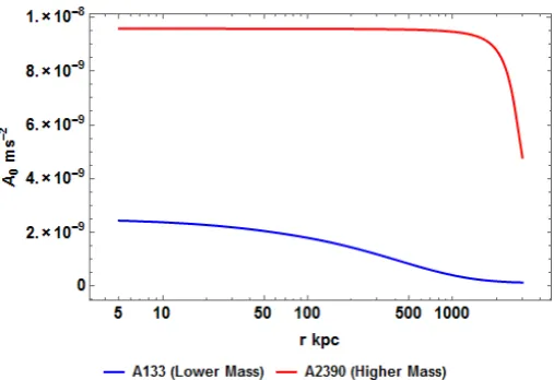
In Figure 4 we plot the calculatedA0as a function of radius for two clusters, A133 and A2390. We choose these two as A133 is a less massive cluster and A2390 is the most massive cluster. We can see that in A2390 the value ofA0is mostly at the maxi-mum value that Equation 20 allows as it has a large gravitational potential, whereas A133 has a much lower A0 which increases towards the centre.

Using this recipe, it is therefore possible to calculate the ef-fective enclosed mass predicted by EMOND for each cluster by which we mean Newtonian mass plus phantom mass,

ME MOND(r)= r2_|∇Φ

E MOND|

G , (21)

where∇ΦE MONDis the gravitational acceleration given by

Equa-tion 17. To accomplish this, we need to solve a first order dif-ferential equation for the potential Φ. This requires a bound-ary condition of the potential. For this we picked three values for the boundary, which we set atrbound = 2r200for each clus-ter. The three values wereΦ(rbound)= ΦNFW(rbound),Φ(rbound)=

0.5ΦNFW(rbound),andΦ(rbound)=1.5ΦNFW(rbound). We did this

for two reasons. First, we would expect that the potential can be approximated by the NFW profile and also we wanted to show how much the calculated mass is affected by the choice of bound-ary potential. In Figures 17 to 22, where we show the results for each cluster using the EMOND recipe, the shaded region high-lights the dependence of the boundary potential.

The final aspect of the EMOND analysis that we should pro-vide for completeness is proving that the EMONDT2term is in fact negligible. To do this, we can solve the right-hand side of Equation 5 by again using the NFW profile as an estimation of the total gravity in the clusters. We can then compare this result to the simplified Poisson equation, Equation 7, to see the effect that theT2 term has on the result. Assuming the simpleµ func-tion (Equafunc-tion 4), asF0(y)=µ(√y),F(y) takes the form,

F(y)=−2√y+y+2 log(1+ √y). (22)

wherey=|∇Φ|2/A0(Φ)2. Therefore,

yF0(y)−F(y)=2

√ y+y

1+√y −2 log(1+ √

y). (23)

11.8 12.0 12.2 12.4 12.6 12.8 13.0 0

2.×10-9

4.×10-9

6.×10-9

8.×10-9

1.×10-8

Log10(ΦNFW) (m2s-2) A0 ( m s -2)

Fig. 3.Plot showing the required value ofA0according to the EMOND

formalism (Equation 18) such that predicted gravitational acceleration from EMOND matches the dynamically calculated acceleration (Equa-tion 12) for each cluster in the sample (thin lines). We plotted this re-quiredA0against the NFW gravitational potential as a estimation of the

behaviour within the cluster. The shape takes the form of an exponential function overplotted in red and described by Equation 19. Also plotted in blue is the more complicatedA0 function described by Equation 20

with a parameter choice,Φ0 = −27000002 m2s−2 and A0max = 80a0.

Note the apparent turnover ofA0at the deepest potential is an artefact

because the total gravitational potential is not just that of an NFW pro-file as assumed here.

Fig. 4.Plot showing the calculatedA0for 2 clusters, A133 and A2390,

using Equation 20. Note that unlike A133, the massive A2390 has a potential mostly above the step function, hence shows little dependence on the changing of the boundary potential (cf. Figure 16).

Assuming the simpler case whereA0(Φ)=a0exp(Φ/Φ0),

d(A0(Φ))2

dΦ =

2a2₀ Φ0

exp 2Φ

Φ0 !

. (24)

We now have all the ingredients to numerically plot the T2 term. To accomplish this, we show, for conciseness, the result for one cluster, A133, as an example but all clusters show sim-ilar results. In Figure 5 we plot the full right-hand side (RHS) of Equation 5 and the RHS of 7. This is essentially a plot of the predicted Newtonian density profile from the EMOND formu-lation with theT2term included and neglected. We see that the plot shows that the results are almost identical and thus we were justified in neglecting theT2term in our previous analysis. The values deviate from each other in the outer radii of the cluster. This is because the NFW profile is not a perfect solution of the EMOND equation and the predicted Newtonian density falls to

Fig. 5.Plot showing the calculated density, predicted by EMOND for cluster A133. Blue dashed line shows the density with the inclusion of theT2term (Equation 5) and red line shows the density calculated from

approximate Poisson equation (Equation 7). The lines are almost iden-tical showing theT2 term was indeed justifiably neglected. Note that

the small differences in the outer regions of the cluster is an artifact be-cause the asymptotic potential of NFW is compatible mathematically with EMOND only if the latter also allows the density dipping into neg-ative at large radii.

zero and eventually negative. The difference in the two lines is just a result of the small delay between the two terms driving the density to this zero point.

We conclude from this analysis that EMOND has had mixed success as a MOND generalization to explain the missing mass in galaxy clusters. We therefore look for an alternative in the following section.

5. An empirical alternate formulation explaining the mass discrepancy

Despite the mixed success of EMOND in answering the question of missing mass in galaxy clusters, the trend of missing mass versus gravitational potential seems to linger. Also the idea of having a0 as a non-constant function may not sit comfortably with the MOND community. This prompted us to look for a dif-ferent formalism that could unify galaxies and galaxy clusters with one law. We thought it would be a good idea to determine the residual in the MOND formula, which we will call B, to de-termine if there is some common theme throughout the clusters. The MOND residual is found by rearranging the MOND formula such that,

B=|∇ΦN| |∇Φ| −µ

|∇Φ|

a0 !

, (25)

which is just moving everything in Equation 2 to one side, as-suming spherical symmetry. The hope here was that we could find a function for B that is 0 in galaxies, thus preserving reg-ular MOND, but non-zero in galaxy clusters. We can determine whether there is a trend if we plot the value of B for each cluster in our sample, assuming that the total gravitational acceleration is approximated by the best-fit NFW profile as a function of total gravitational potential of each cluster; this gravitational potential is also approximated by the gravitational potential of the NFW profile. With this approach, we attempt to determine whether

12.0 12.2 12.4 12.6 12.8 13.0 13.2

-1.0

-0.8

-0.6

-0.4

-0.2 0.0

Log10(ΦNFW) (m2s-2₎

B

Fig. 6.Plot showing the quantity B (Equation 6) vs. NFW gravitational potential for each cluster. By approximating the total cluster gravity as that of the NFW halo, we illustrate that any correction term B to the regular MOND formula, while having a trend with the potential of each cluster, cannot describe all clusters simultaneously.

12.0 12.2 12.4 12.6 12.8 13.0 13.2

-1.0 -0.8 -0.6 -0.4 -0.2 0.0

Log10(ΦNFW) (m2s-2)

B2

Fig. 7.Plot showing the valueB2(Equation 26) as a function of NFW

gravitational potential for each cluster (thin lines). We overplot a thin blue line that showsµ(Φ/Φ0) forΦ0 = −17000002 m2s−2. Note all

clusters lie fairly close to this line, with some discrepancy due to our adopted NFW profile not representing the total potential. ThisB2

cor-rection to MOND allows the MOND interpolation function to run with the potential as well as the acceleration.

there is an additive component to the original MOND formula that can boost the gravity inside clusters, whilst preserving reg-ular MOND in galaxies. We plot this result in Figure 6.

One may notice that although there is not a single function that could fit all these clusters, there seems to be some regularity to the plot. To determine whether the result in Figure 6 can be improved, we tried modifying our Equation for B (Equation 25) slightly such that,

B2 = |∇Φ_N|

|∇Φ| −µ |∇Φ|

a0 + Φ Φ0 !

. (26)

5.1. Summarizing and refining the formulae

Analysing the data seems to show a possible alternative formu-lation of MOND that could account for the mass discrepancy in this sample of clusters. The modified empirical relation in this case would be

|∇Φ_N| |∇Φ| −µ

|∇Φ|

a0 +_ΦΦ

0 !

=B2(Φ), (27)

where the gravitational potential,Φ, and scale potential,Φ0, are negative quantities. As we have seen in Figure 7, B2 looks like a MOND interpolation function,B2(Φ)=µ(Φ/Φ0(Φ)). Im-plementing this, our new modified MOND function is written as

∇ΦN =

"

µ |∇Φ|

a0 + Φ Φ0 !

−µ Φ Φ0

!#

∇Φ, (28)

whereΦ0is our scale potential analogous to the MOND acceler-ation scalea0.

Equation 28 is a relation based on the MOND paradigm, which in the future can hopefully lead to a gravity theory that can explain away the mass discrepancy in galaxy clusters whilst preserving the dynamics of galaxies.

We have yet to mention the value for the scale poten-tial Φ0. For our results, we chose a scale potential of |Φ0| = 17000002_m2_s−2_{. We do not attempt to perform a rigorous Monte} Carlo search over the parameter space in this work as we feel that to do this properly would require some independent tests of the equations such as gravitational lensing and Milky Way data to ensure our parameter does not cause contention with local ob-servations. This is best left for further work.

5.2. Comparison to MOND

We do however show a plot showing how the interpolation func-tion of our relafunc-tion compares with that of regular MOND (Figure 8). Here,

µNew=

"

µ |∇Φ|

a0 +_ΦΦ

0 !

−µ Φ Φ0

!#

(29)

and

µMOND=µ |∇Φ|

a0 !

. (30)

We compare Equations 29 and 30 in Figure 8, assuming that the potentialΦ = Φextas defined in Section 2.3 for different

val-ues of accelerationaranging from 0.01a0−100a0. We also show rotation curves for two galaxies, M33 and NGC4157, using the new relation and EMOND (Figures 9 and 10). These rotation curves have been used in Sanders (1996) for M33 and Sanders & Verheijen (1998) for NGC 4157. We overplot the MOND pre-diction for comparison. There is little deviation from MOND for these two examples. There may be some degeneracy between fit-ting the scale potential for a galaxy and the stellar mass to light. We do not discuss this point here, but mention it as a possible avenue for future work. We have used a fixed background po-tential for both galaxy cases whereas in practice, this may not

0.01 0.10 1 10 100

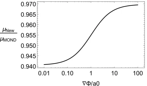
0.940 0.945 0.950 0.955 0.960 0.965 0.970 ∇Φ/a0 μNew μMOND

Fig. 8.Plot showing how the MOND interpolation function and the in-terpolation function of our relation (Equations 29 and 30) compare for a low potential object (Φ = Φext) for different values of acceleration. We can see little variation, which is ideal for preserving galaxy physics with this new relation.

be correct. Ideally one would make a larger scale simulation en-compassing a large area of space and work out the external po-tential (and field) for each galaxy. This was mentioned in (Haghi et al. 2016) who used the external field to explain declining ro-tation curves. They also mentioned that this was now possible thanks to the MOND patch in RAMSES, Phantom of RAMSES (Teyssier 2002) and (Lüghausen et al. 2015). This would require more work to incorporate for example EMOND as the gravity solver would need to be altered to allow varyinga0values.

6. Comparing the new relation to the NFW fits

In this section, we provide plots of the dynamical mass, the mass predicted by invoking the new relation andΛCDM predictions for the 12 clusters outlined in Section 3. The dynamical mass is calculated via Equation 12, the mass predicted from the new relation,

MNew(r)=

r2∇ΦNew

G (31)

where∇ΦNewis calculated via Equation 28 and theΛCDM mass

from,

M_ΛCDM(r)=Mgas(r)+MBCG+MNFW(r). (32)

The NFW parameters used in Equation 32 are taken from (Vikhlinin et al. 2006) and are displayed here in Table 4 in which the NFW mass is defined as

MNFW(r)=4πρsr3s

"

ln 1+ r rs

!

−

1+rs

r −1#

, (33)

whereρs andrs are the scale potential, and radius of the NFW

profilersis defined asrs = r500/c500, where the values forr500 andc500(the NFW concentration parameter) can be found in Ta-bles 3 and 4, respectively. The valueρs is calculated from the

equation,

ρs=

500 3

r500 rs

!3 _ρ

crit

logh1+r500_r s

i

−h1+ rs

r500

i−1, (34)

20 40 60 80 100 120

Velocity

(

km

s

-1)

M33

0 2 4 6 8

0 0.5 1. 1.5

Radius(kpc)

Velocity

Residule

(

km

s

-1)

Fig. 9.Top plot showing the rotation curve of M33. Blue points are the data with error bars, the black dashed line is the regular MOND fit, the red line is the new relation, and the blue line is EMOND. In the bottom plot we also show the residual between MOND, the new relation, and EMOND. Note the difference between these rotation curves are actually tiny (∼1km/s). Here we adopted a background potential of 10−6_c2_given

in Zhao & Famaey (2012)), and a stellar mass to light of 0.722.

Table 4.NFW concentration parameters at radiusr500. NFW profiles

can be determined by combining these with ther500parameters given in

Table 3, the values forrsand the value forρsgiven in Equation 34.

Cluster c500

A133 3.18

A262 3.54

A478 3.57

A1413 2.93

A1795 3.21

A1991 4.32

A2029 4.04

RXJ1159 1.7

MKW4 2.54

A383 4.32

A907 3.48

A2390 1.66

whereρcritis the critical density.

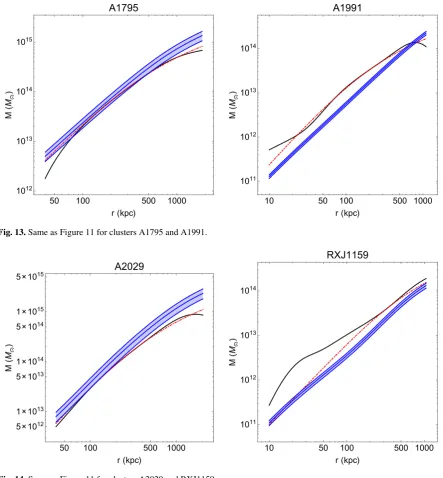
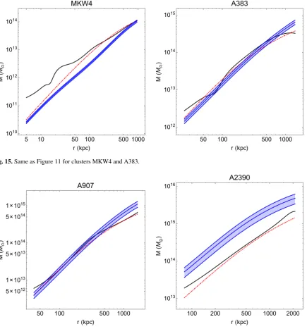
We can see from the dynamical mass plots (Figures 11-16) for each cluster that on average the new relation can provide a reasonable boost, or at least a reasonable match to the NFW pro-file, for the sample. The most noticeable outlier from our new relation is A2390, which has a very poor fit. A2390 is the largest cluster and thus has the largest gravitational potential. This new relation, in this current from, has a problem in very high

gravita-80 100 120 140 160 180 200

Velocity

(

km

s

-1)

NGC4157

5 10 15 20 25

1 2. 3 4

Radius(kpc)

Velocity

Residule

(

km

s

-1)

Fig. 10.Same as Figure 9 for galaxy NGC4157. We use a stellar mass to light of 1.69 for each case.

tional environments (see Section 7). Perhaps a refinement of the formalism in these high potential regions may solve the problem of A2390. We also acknowledge that a rigorous error analysis has not been performed and thus it is hard to gauge how well this new relation has faired in predicting cluster masses.

Also, we do not truncate the gas density in our calculation. It is unrealistic that the gas density extends tor200. As we do not have the necessary data to constrain this, we also leave this as an open issue.

7. Limitations of the new relation and required testing of the formalism

Although the new relation can recover the mass of the cluster to reasonable precision, there is a severe flaw in the empirical law. Both the gravitational potential and acceleration are large near stars and black holes. Therefore we have |∇_a0Φ| + _ΦΦ

0 >> 1 and

Φ

Φ0 >>1. This results in

"

µ |∇Φ|

a0 + Φ Φ0 !

−µ Φ Φ0

!#

→1−1→0. (35)

and thus Equation 28 becomes,

∇Φ =∇Φ_N/0→ ∞. (36)

to the structure of Equation 28, which has one interpolation function subtracting another. Perhaps when constructing a La-grangian based formulation of the law, there will arise some ex-tra terms that could counter this problem. This is an issue which is not addressed here, but in further work.

Despite these two issues, it is still possible to further test this law with regard to gravitational lensing and by looking at the dynamics of objects within clusters, which will be affected by the external potential effect. Possible candidates for the latter could be rotation curves for intercluster galaxies or the mass estimates for the newly discovered ultra-diffuse galaxies (Beasley et al. 2016), all of which are beyond the scope of this work.

Finally, more rigorous data analysis should be conducted to determine whether better interpolation functions can be found and a parameter search could be implemented to determine better model parameters.

8. Discussion and conclusions

In this work, we look at the possibility that the missing mass in galaxy clusters, which is still present in MOND, may be at-tributed to a modified gravity law that is a generalization of MOND. Beginning with an overview of a previous study con-cerning this area, we review the equations of EMOND and ap-ply the formalism to a sample of galaxy clusters. We show that EMOND in its current form has partial success in explaining the clusters.

We then go on to use the data to determine if there is any empirical relation that could explain the missing mass in galaxy clusters. We find that there is such an expression, which works relatively well for this sample of clusters. The new formula has the ability to account for the missing mass in clusters by modify-ing the MOND formula in such a way that the gravity is boosted in regions of high gravitational potential whilst preserving the regular MOND formula in regions of weak gravitational poten-tial.

The main issue with this modified equation however, is that in regions of high acceleration and high potential, such as near a star or black hole, the enhancement of gravity calculated with the formula tends to infinity and is thus in contradiction with ob-servation. A thorough investigation is also needed to refine the interpolation functions and the new scale potential value by ex-panding the data set of clusters and invoking new tests of the law, such as gravitational lensing and dynamics of objects that lie within galaxy clusters. Furthermore, the empirical equations here should have a Lagrangian formulation, which would also have implications for cosmology. While it is difficult to predict the applications of our model to cosmology partly because of the lack of a covariant Lagrangian, the effect of a lower MOND ac-celeration scale in galaxies compared to galaxy clusters in our model could mean that the structure formation is suppressed in galaxy scale compared to cluster scale. This might skew the rel-ative abundances of bound systems and suppress the luminosity functions at the lower end.

It is very difficult at this stage to speculate on any implica-tions for cosmology and structure formation with the new re-lation we describe as it still has theoretical challenges. We can however make some comments with regards to EMOND. Firstly, there is a known connection between dark energy and MOND: mainly, (8a0)2/(8πG) ≈Λ. If, like in EMOND,a0is increased, and there is a link between the acceleration scale factor and dark energy, then EMOND may affect the dark energy contribution and would also imply that the contribution is uneven rather than constant. This could cause differences in late time expansion

and also the angular size of the CMB peaks compared to reg-ular MOND. We would also expect that lensing would be en-hanced if a covariant version were formulated. The main test for EMOND would be the lensing signature of the bullet cluster. Zhao & Famaey (2012) discuss lensing of a bullet cluster-like object in their original work. They find that it is possible to cre-ate phantom dark matter-like effects offset from the baryons in EMOND. Originally, Zhao & Famaey (2012) only boosted the acceleration of the scale factor by a factor of≈6,where as we make a much larger boost of a factor≈50. We should therefore expect larger effects than in the original work. Clearly, to make a stronger case, we would actually have to make a non-spherical model to see if EMOND is in fact consistent with the bullet clus-ter (and train wreck clusclus-ter). With regards to galaxy formation, we might expect galaxies to form differently within clusters as the effective a0 is larger. We mentioned earlier that the nature of the UDGs might be compatible with an EMOND-like theory; perhaps simulations in EMOND could produce these objects. We might also expect that galaxies form differently near the centre of a cluster compared to at the edge asA0(Φ) is very different in the centre than at the cluster edge. One prediction might be that UDGs at the cluster edge should show a less severe dynamical M/L ratio than those closer to the centre.

All these are beyond the scope of our work here, which is to show that there could be an empirical gravity relation that can, without actually invoking dark matter, account for the missing mass in galaxy clusters

ACKNOWLEDGEMENTS

We would like to thank Benoit Famaey for useful discussions. AOH is supported by Science and Technologies Funding Coun-cil (STFC) studentship (Grant code: 1-APAA-STFC12). We would also like to thank the referee for very useful comments and Anne-Marie Weijmans for proofreading the draft.

References

Angus, G. W. 2009, MNRAS, 394, 527

Angus, G. W. & Diaferio, A. 2011, MNRAS, 417, 941

Angus, G. W., Diaferio, A., Famaey, B., & van der Heyden, K. J. 2013, MNRAS, 436, 202

Angus, G. W., Famaey, B., & Buote, D. A. 2008, MNRAS, 387, 1470 Beasley, M. A., Romanowsky, A. J., Pota, V., et al. 2016, ApJ, 819, L20 Bekenstein, J. & Milgrom, M. 1984, ApJ, 286, 7

Bekenstein, J. D. 2004, Phys. Rev. D, 70, 083509

Blanchet, L. 2007, Classical and Quantum Gravity, 24, 3529 Blanchet, L. & Novak, J. 2011, MNRAS, 412, 2530

Combes, F. & Tiret, O. 2010, in American Institute of Physics Conference Series, Vol. 1241, American Institute of Physics Conference Series, ed. J.-M. Alimi & A. Fuözfa, 154–161

Derakhshani, K. & Haghi, H. 2014, ApJ, 785, 166 Famaey, B. & Binney, J. 2005, MNRAS, 363, 603

Famaey, B., Bruneton, J.-P., & Zhao, H. 2007, MNRAS, 377, L79 Famaey, B. & McGaugh, S. S. 2012, Living Reviews in Relativity, 15, 10 Felten, J. E. 1983, NASA STI/Recon Technical Report N, 84, 18132

Haghi, H., Bazkiaei, A. E., Zonoozi, A. H., & roupa, P. 2016, MNRAS, 458, 4172

Khoury, J. 2015, Phys. Rev. D, 91, 024022

Koda, J., Yagi, M., Yamanoi, H., & Komiyama, Y. 2015, ApJ, 807, L2 Li, B. & Zhao, H. 2009, Phys. Rev. D, 80, 064007

Lüghausen, F., Famaey, B., & Kroupa, P. 2015, Canadian Journal of Physics, 93, 232

Matsakos, T. & Diaferio, A. 2016, ArXiv e-prints [arXiv:1603.04943] McGaugh, S. S. 2005, ApJ, 632, 859

Mihos, J. C., Durrell, P. R., Ferrarese, L., et al. 2015, ApJ, 809, L21 Milgrom, M. 1983a, ApJ, 270, 371

Milgrom, M. 1983b, ApJ, 270, 384 Milgrom, M. 1983c, ApJ, 270, 365 Milgrom, M. 2009, Phys. Rev. D, 80, 123536

50 100 500 1000 1×1012

5×1012 1×1013 5×1013 1×1014 5×1014 1×1015

r(kpc)

M

(

M⊙

)

A133

10 20 50 100 200 500 1000

1011 1012 1013 1014

r(kpc)

M

(

M⊙

)

A262

Fig. 11.Plot showing mass profiles for the new relation for different values for the boundary potential (blue shaded region). Also the plot shows the NFW (red dotted line) and dynamical masses (black solid line) for clusters A133 and A262.

50 100 500 1000

5×1012 1×1013 5×1013 1×1014 5×1014 1×1015 5×1015

r(kpc)

M

(

M⊙

)

A478

50 100 500 1000

1012

1013

1014

1015

r(kpc)

M

(

M⊙

)

A1413

Fig. 12.Same as Figure 11 for clusters A478 and A1413.

Milgrom, M. 2010, MNRAS, 403, 886

Navarro, J. F., Frenk, C. S., & White, S. D. M. 1997, ApJ, 490, 493 Sanders, R. H. 1996, ApJ, 473, 117

Sanders, R. H. 1999, ApJ, 512, L23 Sanders, R. H. 2003, MNRAS, 342, 901

Sanders, R. H. & McGaugh, S. S. 2002, ARA&A, 40, 263 Sanders, R. H. & Verheijen, M. A. W. 1998, ApJ, 503, 97 Schmidt, R. W. & Allen, S. W. 2007, MNRAS, 379, 209 Teyssier, R. 2002, A&A, 385, 337

van Dokkum, P., Abraham, R., Brodie, J., et al. 2016, ApJ, 828, L6 Vikhlinin, A., Kravtsov, A., Forman, W., et al. 2006, ApJ, 640, 691 Zhao, H. 1996, MNRAS, 278, 488

Zhao, H. 2007, ApJ, 671, L1

50 100 500 1000 1012

1013

1014

1015

r(kpc)

M

(

M⊙

)

A1795

10 50 100 500 1000

1011 1012 1013 1014

r(kpc)

M

(

M⊙

)

A1991

Fig. 13.Same as Figure 11 for clusters A1795 and A1991.

50 100 500 1000 5×1012

1×1013 5×1013 1×1014 5×1014 1×1015 5×1015

r(kpc)

M

(

M⊙

)

A2029

10 50 100 500 1000

1011

1012

1013

1014

r(kpc)

M

(

M⊙

)

RXJ1159

Fig. 14.Same as Figure 11 for clusters A2029 and RXJ1159.

5 10 50 100 500 1000

1010

1011

1012

1013

1014

r(kpc)

M

(

M⊙

)

MKW4

50 100 500 1000

1012 1013 1014 1015

r(kpc)

M

(

M⊙

)

A383

Fig. 15.Same as Figure 11 for clusters MKW4 and A383.

50 100 500 1000 5×1012

1×1013 5×1013 1×1014 5×1014 1×1015

r(kpc)

M

(

M⊙

)

A907

100 200 500 1000 2000 1013

1014

1015

1016

r(kpc)

M

(

M⊙

)

A2390

50 100 500 1000 1×1012

5×1012 1×1013 5×1013 1×1014 5×1014 1×1015

r(kpc)

M

(

M⊙

)

A133

10 20 50 100 200 500 1000

1×1011

5×1011

1×1012

5×1012

1×1013

5×1013

1×1014

r(kpc)

M

(

M⊙

)

A262

Fig. 17.Plot showing mass profiles for the EMOND relation for different values for the boundary potential (blue shaded region). Also the plot

shows the NFW (red dotted line) and dynamical masses (black solid line) for clusters A133 and A262.

50 100 500 1000

5×1013

1×1015

r(kpc)

M

(

M⊙

)

A478

50 100 500 1000

1012

1013

1014

1015

1016

r(kpc)

M

(

M⊙

)

A1413

Fig. 18.Same as Figure 17 for clusters A478 and A1413.

50 100 500 1000 5×1012

5×1013 5×1014 5×1015

r(kpc)

M

(

M⊙

)

A1795

10 50 100 500 1000

1011

1012

1013

1014

r(kpc)

M

(

M⊙

)

A1991

Fig. 19.Same as Figure 17 for clusters A1795 and A1991.

50 100 500 1000

1013

1014

1015

1016

r(kpc)

M

(

M⊙

)

A2029

10 50 100 500 1000

1011

1012

1013

1014

r(kpc)

M

(

M⊙

)

RXJ1159

5 10 50 100 500 1000 1010

1011

1012

1013

1014

r(kpc)

M

(

M⊙

)

MKW4

50 100 500 1000

1012

1013

1014

1015

r(kpc)

M

(

M⊙

)

A383

Fig. 21.Same as Figure 17 for clusters MKW4 and A383.

50 100 500 1000 5×1012

1×1013

5×1013

1×1014

5×1014

1×1015

r(kpc)

M

(

M⊙

)

A907

100 200 500 1000 2000

1013 1014 1015 1016

r(kpc)

M

(

M⊙

)

A2390

Fig. 22.Same as Figure 17 for clusters A907 and A2390.