Stability evaluation of a DC micro grid and future interconnection to an AC system

Stability evaluation of a DC micro-grid and future interconnection

to an AC system

a,*, a a,b

Santiago Sanchez

Marta Molinas , Marco Degano

, Pericle Zanchetta

b

aDepartment of Electrical Power Engineering, Norwegian University of Science and Technology, Trondheim NO 7491, Norway bDepartment of Electrical and Electronic Engineering, University of Nottingham, University Park, Nottingham, UK

a b s t r a c t

This paper presents the stability analysis of a DC micro-grid fed by renewable sources and the future interconnection with an AC micro-grid. This interconnection is realized through a voltage source con-verter, and the operation of the micro-grid is in island mode. The stability is analyzed by the Nyquist criteria with the impedance relation method. The frequency response of the models was obtained by the injection of a perturbation current at the operation point. Where this perturbation was at the input of the converter used to export power from the DC grid. Other perturbation was applied at the node of the micro-grid to evaluate its impedance. Finally the simulations show the impedance representation of the systems, and the stability for the interconnection of them. The experimental verification shows the impedance of the converter with the same tendency as the representation obtained by the analytical and simulation.

1. Introduction

The stable behavior is one of the most important factors in po-wer systems. Its correct analysis ensures to the designer or operator that the system is going to be under normal conditions. Small signal techniques were developed for classical power systems, where generator to load currentflow is always assumed[1]. But, future grids can present a system with power injection into the grid from the side of the costumer. These future grids will exhibit more nonlinear behavior and difficult coordination than the classical power system. In the case of DC distributed power electronics systems used in telecommunications, aircraft or ships the stability had been studied in Refs.[2e5]. Where stable region operation was identi_fied. These methods employ frequency response and Nyquist criteria to present stability analysis. Linearization has been done, due to its simplicity and success record [6,7]. The wide spread choice to predict instability by the application of small signal analysis such as the Nyquist criterion or eigenvalues in AC systems with power electronics has been presented in Refs. [1,8e14]. However, it is necessary to analyze the stability of the distribution system with one of its prominent topology, in this work it is

presented a variant of the CIGRE AC benchmark[15]for a DC resi-dential low voltage micro-grid, and its stability has been studied at one of the power exchange nodes.

The paper is organized as follows: the Section2describes the modeling by impedance representation, Section3presents the grid structure and the method employed to control the DC voltage, and Section 4 describes the numerical results obtained from the simulations.

2. Impedance representation methods

voltage type and a Norton equivalent system in which the source is considered current type, as is shown inFig. 2. For voltage source type the analysis has to be realized over the Thevenin circuit and the voltage applied to the load subsystem is calculated in(1), where VLis the voltage in the load,Zs is the output impedance of the source, andZLis the input impedance of the load.

VL ¼ 1 1þZs

ZL

The relationZs/ZLis used to realize the stability analysis, if its Nyquist plot counterclockwise encircles the point1þj0 then the system has an instability. And in case of use the Norton equivalent circuit the current in the loadILis(2), whereIsis the source current.

Vs (1)

IL ¼

1 1þZL

Zs

Is (2)

2.1. Voltage source converter

The system used to interconnect the two grids is a power electronics three phase voltage source converter (VSC). This device operates as a rectifier and is used to link the two systems. The equations of a voltage source converter connected at the DC side to a grid and to an ideal AC system are described from(3)e(6).

did E v þwLiqrid

dt ¼ L

sd d ₍₃₎

diq EsqvqwLidriq

dt ¼ L (4)

dv_dc dc igrid

dt ¼ C

i þ

(5) 2.3. Linearization and transfer functions relation

i_dc ¼ s i_gddþsgqiq (6)

whereEs,kwithk˛{d,q} is the voltage of the AC grid in the direct and quadrature axis, respectively. The current in thefilter induc-tanceLisik. The voltage at the switch terminals of the converter is vk. The DC voltage isvdc, the current at the DC side of the converter isidc, the switching commands aresgk, and the currentflowing from the DC grid isigrid. The controller for this system is design with the

set of equations from(7) to (11).

v_d ¼ kp i_refdi_d k_i

g

dþwLiq

a

e Esd (7) _{final model is shown in(19).}

at

vq ¼ kp _refqiq _q Esq (8)

i ki

g

wLid

a

eat

_ ¼ i id (9)

g

d refd

_ ¼ i iq (10)

g

q refq

sgk ¼ vk (11)

vdc

The impedance of the load or converter connected to the grid can be estimated by the use of three techniques. They are described in the followed subsections.

2.2. State space linearization

The nonlinear function(12)can be linearized around an oper-ation point and the system described by(13) and (14). For the converter the low frequency impedance is obtained by the method described in Ref.[14], the current of the source (or DC grid at the node) is the input to the system, the states are the AC currents, and the voltage in the DC capacitor; that is chosen as the output of the system. The matrix form of the differential equations for the inverter is(3) and (6).

_

x ¼ fðx;uÞ (12)

D

x_ ¼ A

D

xþB

D

u (13)

y¼ Cm

D

x (14)

For this method the input is equal to the grid currentu¼igrid, the states arex¼(id,iq,vdc,

g

d,

g

q)T. The impedance in the frequency domain is calculated with(15).

1

Z_dcðsÞ ¼ CmðsIAÞ B (15)

The impedance obtained by this method is:

2

ZdcðsÞ ¼

ðsþ

a

Þv_dc

s2Cv2 þsCv2

a

i ki

g

ðsþ

a

Þ þ

dc dc d d id

a

Esd

(16)

To obtain the impedance representation by this method the steps used in Refs. [16,17], are described to be applied over the model of the set(3)e(11). First the models are obtained in the time domain. In the second step, the Laplace transform is realized for the states in order to obtain the transfer functions. A linearization around the operation is required in this step. The transfer function that represents the impedance is obtained by the relation between the variablesvdcandidcin Laplace domain. And the impedance of the full converter is obtained by the equivalent parallel between DC capacitance and the impedance of the converter. The obtained impedance for this system is presented from(17) and (18), and the

ZvscðsÞ ¼ vdc vdcðrþsLÞ ðsþ

a

Þ2

idc 4 3 2 1 a0 2

a s4þa s3þa s2þa sþ

!

(17)

a_k ¼ fk Kptrans;Ga;x0 ; k˛f0;.4g (18)

Z_dcðsÞ ¼ ZCðsÞZvscðsÞ

[image:2.595.59.259.66.126.2]

ZCðsÞ þZvscðsÞ (19)

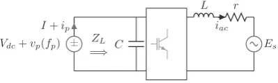
[image:2.595.35.280.631.728.2]

Fig. 1.Perturbation source for impedance measurement.

where Kptransis the gain of the power from the abc to the dq reference frame,Ga¼1/Vdcat the nominal value, the parametersak are described in theAppendix A,ZCis the impedance of the DC capacitor.

2.4. Harmonic balance principle

The harmonic balance[18,19]is used to obtain the impedance by injecting a perturbation into the converter at the DC side and see its effect at the AC side. The approximation is obtained by the assumption employed in Refs.[20,21], which use no energy stored in thefilters of the DC and AC side, it can be seen in(20).

vdcðtÞidcðtÞ ¼ vaðtÞiaðtÞ þvbðtÞibðtÞ þvcðtÞicðtÞ (20)

whereva,b,c(t),ia,b,c(t) are the voltage, and current for the AC side respectively, andvdc(t) is presented as a time variable signal like

(21)in order to include a sinusoidal perturbation voltage applied from the DC side to obtain the small signal impedance. Then, the currentidc(t) at the DC side is expected to be time variable.

vdcðtÞ ¼ VdþVpcos t (21)

whereVd,Vpare the constant component, and the perturbation

maximal value,

u

pis the angular velocity of the perturbation signal. In order to evaluate the left hand side of(20), the time variable DC current is assumed as in(22)with a constant componentId, a

perturbation valueIp, and a lagged angle4p.

idðtÞ ¼ IdþIpcos

up

t

fp

(22)

up

The evaluation of(21), and(22)in the left hand side of(20)is presented in(23).

p_dcðtÞ ¼ I V_{d d}þ21IpVpcos

f

_p þIdVpcos

up

tþ

IpVdcos

up

t

fd

þ1IpVpcos2

up

t

fd

2

(23)

The PWM signals are obtained by comparing a triangular waveform vtri(t) with peak value Vtri and the control voltages

vCk(t)¼VCcos(

u

et

g

k) in whichk¼{a,b,c} and

g

k¼{0, 120, 240} degrees for its respective phase; where the duty ratios in the average representation can be written as is shown in(24) [21].

dkðtÞ ¼ 0:5þ0:5

VC

V_tricosð

ue

t

g

kÞ (24)

Using the duty ratios of(24)and the time variable DC voltage to obtain the phase to DC neutral voltages(25), and(26)are obtained.

v_kNðtÞ ¼d_kðtÞv_dcðtÞ (25)

v_kNðtÞ ¼Vd VdVC Vp

2þ2Vtricosð

ue

t

g

kÞ þ 2

cos

up

t

þVpVC (26)

8Vtri

2cos weþwp t

g

k

þ2cos wewp t

g

k

The terms 0.5Vd, and 0.5Vpcos(

u

pt) in(26)are offset voltages, and in each phase are considered as zero-sequence voltages as is analyzed in Ref.[21]for the term 0.5Vd, therefore do not produce currentflow in the balanced three phase load. Then the average

phase to neutral voltages for the balanced star load with neutraln, are as in(27).

V_dVC VpVC v_knðtÞ ¼

2Vtri 4Vtri

cosð

ue

t

g

kÞ þ cosweþwpt

g

k

þcos wewp t

g

k

(27)

In(27)there are three frequency components and each signal has its respective maximum value. To facilitate the use of(27), it is written as(28), whereV1sV2, andV2¼V3.

v_knðtÞ ¼ V1cosð

ue

t

g

kÞ þV2cos weþwpt

g

k

þV3coswewpt

g

k (28)

Assuming that the system has a linear part the currents in each phase are expected to have the same frequency components that the voltages, and its respective lagged load angle. Also, the magnitude of the current in its respective frequency is assumed to be proportional to the magnitude of the impedance at the same frequency. Hence the current in each phase is(29).

i_knðtÞ ¼ I1cosð

ue

t

g

k

f1

Þ þI2cos weþwp t

g

k

f2

þI3coswewpt

g

_k

f3

(29)

The magnitudesI1,I2, andI3in(29)are functions of the three phase balanced impedance that is a function of the frequency, and is notated asZ1(

u

e), Z2(

u

eþ

u

p), andZ3(

u

e

u

p). Therefore, the

angles of the load are

f

1(

u

e),

f

2(

u

eþ

u

p), and

f

3(

u

e

u

p).

The controller can be added assuming that there is a PI regulator in the converter, the reference current can be model by irefRk ¼Irefcos(

u

t

f

1

g

k), the integrated reference current is i_refk ¼ ðI_ref=

uÞ

sinðut

f

1

g

kÞ. The controller is applied into

refk

the variableVCfor each phase as follows:

VCk ¼ kp irefkikn þki irefkikn dt (30)

Z

Equations(28)e(30)are used in the right hand side of(20)to obtain the AC power(31)at the injected perturbation frequency and to build the model that describes the impedance.

pacwpt ¼ Kpac kpf1power

up

tþkif2power

up

t (31)

where Kpac is the gain of the power obtained. The functions

flpower(

u

p) withl˛{1, 2} describe the power functions obtained for the proportional and integral controller, respectively. The equation

(31)is compare with the fourth term of(23)in order to obtain an expression forip. Then, tofind the value ofIpas a function of the AC impedance in frequency a complex notation is used in(32)e(38).

2 3 2 3 jf1

Ip;kp ¼ kp I3 wewpwe þI2 wewpwe I1e (32)

I_p;ki ¼ ki I3b wewpw2e þI2b wewpw2e I1ejðf1þp=2Þ

(33)

I2 ¼ I2ejf2 (34)

I_2b ¼ I2ejðf2þp=2Þ (35)

I3 ¼ I3ejf3 (36)

Ip ¼

Ip;kpþIp;ki

V_tri w_ewew2_p

3 (38)

The next step is to compute the impedance by the relation presented in(39).

Z_dcð

u

Þ ¼ Vpð

u

Þ

Ipð

u

Þ (39)

Finally, the complete converter impedance is found by the par-allel of the capacitor and(39).

3. Grid topology

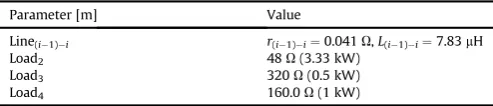
The topology described inFig. 3is based on a segment of the CIGRE benchmark low voltage micro-grid[15], with some modifi -cation to operate with direct current, and a voltage of 400 V DC. The line parameters are calculated for a service connection feeder 16 mm2Cu. Also, they are described inTable 1, Loadirepresents the load in the nodei, the line between the nodes is Line(i1)i, and its resistance and inductance values are r and L, respectively. The distance between each node is 30 m. The system is composed by a wind turbine (WT) with 5 kW of power (DG1), with a permanent

magnet generator, a diode bridge rectifier, followed the DCeDC converter. The second renewable source (DG2) is a photo-voltaic (PV) 5 kW system operating in maximum power extraction and a DCeDC converter to regulate the voltage supplied to the grid. The third distributed generator is a battery bank (ES) which contributes in the power sharing, and is coupled to the grid by a DCeDC bidi-rectional converter. The power can be exported or imported by a voltage source converter (Pex) connected to an AC system. Where the coordination of the grid has been realized with power sharing by drop controlPeV, and one operation point is used for the sta-bility test.

3.1. Wind turbine model

The small power turbine is modeled and controlled as in Ref.

[22]. A description of the dynamic system is described in the fol-lowed subsections.

3.1.1. Wind turbine

A simplified model that shows the relation between the wind velocity, the generated power (Pm) and rotational speed (

u

) is

described in(40).

Pm ¼ 1

r

Cpð

l

;

b

ÞAwV3

2

where

r

is the air density,

b

is the pitch angle which is chosen as zero for small power turbines,Awthe area covered by turbine,Vwis

the wind speed,

l

is the tip speed ratio defined in(41),

u

rrotor angular velocity, and

F

is the turbine blades diameter.

w (40)

l

¼

ur

Vw 2

F

(41)

Cpð

l

Þ ¼ 0:5 5 e

116

l

i

21

li þ₀:₀₁

l

₍₄₂₎

with

l

idescribed in(43).

1

l

i ¼

_l

0:03 (43)

A one mass model describes the dynamics of the mechanical speed(44).

1

d

ur

1

dt Jm

whereJmis the electrical machine and turbine inertia coefficient,TE

electrical torque and the mechanical torque is defined as(45).

¼ ðTmTEÞ (44)

Tm ¼ Pm

ur

(45)

3.1.2. Permanent magnet synchronous generator

A model in the space vector representation is presented in this work [23], the system is described in (46)e(48) as generator operation. The parameters of the machine are npthe pole pairs number,Ls,Rsthe stator inductance and resistance respectively,J

the inertia coefficient of the machine,is,vsthe stator current and voltage respectively,

F

mmagnetizationflux, and

q

rrotor angle.

d

Ls is ¼ RsisþjnpurFme

dt

jnpqr_{vs (46)}

ur

¼ Tm

Fm

Imag

Jd ise (47)

dt

h n oi

jnpqr

d dt

whereImag{} is the imaginary part, the space vector notation for the stator current and voltage as described in (49) and (50), with

g

k¼{0, 2

p

/3, 4

p

/3},ik(t), andvk(t) the phase current, and voltage respectively.

qr

¼

ur

(48)

is ¼ i ðtÞe (49)

[image:4.595.299.549.494.585.2]

Xc

Table 1 k¼a

Line parameters for the micro-grid structure.

k jgk

vs ¼ Xv ðtÞe (50)

Parameter [m] Value c

k¼a k jgk

The machine can be seen as a source in series with a resistance and an inductance in the stator, it can be observed inFig. 4.

Fig. 3.DC micro-grid used for the stability test.

Line(i1)i r(i1)i¼0.041U,L(i1)i¼7.83mH

Load2 48U(3.33 kW)

Load3 320U(0.5 kW)

[image:4.595.35.282.687.740.2]

3.1.3. Full bridge diode rectifier

The arrangement of the rectifier is a full bridge, six pulse, and three phase, with a filter capacitor at the DC side. The model description assumes the inductance value at its AC terminals to be zero [20], the instantaneous DC voltagevdc is presented in(51),

whereVLLis the rms line to line voltage value. The direct currentIdc

in function of the peak phase currentImis(52).

v_dcðtÞ ¼ 2V_LLcos

u

t <

u

t< (51) 0 S0

pffiffiffi

_p

_p

T Ak

6 6 Tref

I_dc ¼

ffiffiffi 3 2 p

Im (52)

For the rectifier the DC voltage average valueVdcis(53).

Vdc ¼ 2VLL (53)

3

p

3.1.4. Buck-boost converter model

The Buck-boost structure is chosen for this work due to its operation characteristics. Where the input voltage can be higher or lower than the output voltage. Continuous conduction mode is assumed for the design of the model. In(54)the dynamic of the inductor current (iL1) is presented, with a switching signalq1, the

inductance isL1, and the source voltagevinp1. The dynamic voltage of the capacitance (vo1) is in(55), the capacitance of the converter is Cf1, the parameterio1is output current.

ðq 1Þv þq

pffiffiffi

di_L1 1 o1 1vinp1

dt ¼ _L1 (54)

dv_o1 ð1q₁Þi_L1io1

dt ¼ _Cf1

(55)

The DCeDC structure is presented inFig. 5. An ideal switch (S) is showed in the place of the IGBT[21], and the load resistance isRbb.

3.2. Solar module

[image:5.595.282.528.61.355.2]

The equations that describe the solar cell are described in Refs.

[24,25]. The dynamic is represented from(56) to (62).

i¼ npI_phnpidnpir (56)

iph ¼ ISC0 þCt TTref (57)

S S0

id ¼ I0 e

qvsh

AkT1 (58)

I ¼ I

!3

e (59)

qEg₁₁ T_ref T

ir ¼ vsh

Rsh

(60)

v_sh ¼ v þiRse (61)

ns

T ¼ TaþksS (62)

where the system parameters are:S0is the standard light intensity, Trefthe temperature under standard test conditions,RshandRseare the shunt and series resistances in the solar cell, ISC0the short circuit current of each solar cell at Tref,IS0 the diode saturation

current of the cell atTref,Egis the band energy of the material,Athe ideal factor,Ctthe temperature coefficient, the coefficientksthat defines the light intensity disturbance,vshvoltage at the shunt

resistor, the electron charge isq, the Boltzmann constant isk,Sis the light intensity, the ambient temperature isTa,vis the voltage at the solar module terminals, andiis the output current.

3.3. Dynamic battery model

The battery array is model in(63) and (64) [26]. The intercon-nection is realized by a bidirectional power electronic interface

[24].

SOC ¼ 100 1

0 Z 1

ibdt

B C

B

@ _Q CA (63)

v_b ¼ VoþR i_bbK Q

Qþ ibdt

Z þAe (64)

Z B ibdt

where the parameters are: SOC is the state of charge, vb is the

terminal voltage,Vois the open circuit voltage,ibis the charging current, Q is the capacity, Rb is the internal resistance, A is the exponential zone voltage,B is the exponential capacity,Kis the polarization voltage.

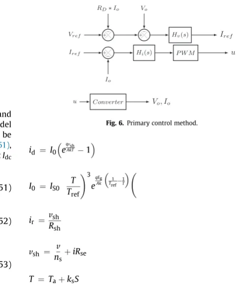
3.4. DCeDC converter control strategy for power sharing

[image:5.595.89.248.65.128.2]

The converters used to keep the voltage constant in the DC micro-grid employ the strategy described in Ref. [27]. Fig. 6 Fig. 4.Permanent magnet machine equivalent circuit.

Fig. 5.DCeDC Buck-boost converter.

describes a primary controller with an inner loop to control the current injected to the system. And an outer loop to control the voltage in terminals of the converter. Hence, is assured the island mode operation and not communication between the sources is required. The grid operates under constant voltage at the point of common coupling with a primary powerevoltage droop controller to realize power sharing[27]. The maximum voltage variation is defined as

D

Vdc¼ 4%. The method is based on the measurement of the voltage and current in terminals of the converter. Where from

Fig. 6,Vref,Irefare the voltage and current references respectively.RD

is a virtual output impedance,Hv(s),Hi(s) are the voltage and cur-rent controllers, respectively. AndVo,Ioare the voltage and current

of the converter.

4. Results

The _first database were created by simulation with the Simulink-Matlab software in order to validate and compare the models obtained by the analytical impedance representation. The symbolic manipulation of the equations was develop with the software Maple, Finally the database for the experimental verifi -cation were stored and manipulated to obtain the impedance with a Matlab script. Hence, the impedances for the VSC were obtained for each method, and the DC micro-grid was calculated by the in-jection of a DC perturbation current at node pcc5inFig. 3plus the operation current that the system is going to have. The node will be used to interconnect the systems, where the converter in this case will export a power of 800 W.Figs. 7 and 8present the impedance behavior of each system.

The frequency analysis for the grid and the VSC impedance is realized with the Thevenin equivalent system. The relation is

presented inFig. 9. Where the stability margin of 6 dB and 30is considered in this work[2]. FromFig. 9is clear that the stability margin is not reached for the frequency range of [10fsw/2] Hz, wherefsw¼10 kHz is the switching frequency used in the VSC. During the tests of the VSC impedance, it is coupled to its AC passive impedance and the DC capacitor. Therefore, the impedance at the DC side is highly affected by the passive systems used[8]. Hence, with the result inFig. 9the system would keep a stable state when is coupled to the DC micro-grid. An improvement in the stability response can be reached by addition of passivefilters, that can shape the_final response as is described in Ref.[16]for an aircraft electric grid. The time domain tests are shown inFig. 10. It presents the transient behavior of the complete grid for small disturbances. When the connection between the DC micro-grid and the AC sys-tem is set it can be seen the damping of the voltage restoration and slow variation in the power shared by the converters. At 1.0s the connection is realized and the systems keep the stability producing a low drop (3%) in the voltage of the grid (vgrid), the operation

voltage is recovered by the action of the droop controller imple-mented in the converters. The power shared is presented inFig. 10, a condition is that the input power to the renewable energy is constant during the time interval studied. Whereppvis the power developed by the solar energy system,pwtis the power from the wind turbine, andpbattis the power from the batteries bank. Finally,

the power drawn by the VSC used to interconnect the DC grid and the AC system ispvsc.

4.1. Experimental verification

The system used to obtain the experimental impedance is described inFig. 11and the test bench picture is shown inFig. 12. The sourcevgenis the perturbation signal with variable frequency

[image:6.595.58.260.65.208.2]

produced by a signal generator(1). This is isolated by a small power transformer and connected to a linear amplifier(2), hence the perturbation is applied to the DC grid by the secondary of the

[image:6.595.327.528.65.141.2]

Fig. 7.Impedance for the VSC system operating at 5%Pn, (*)state space, ()TF, (B) harmonic balance, and (þe) simulation.

Fig. 8.Impedance for the DC micro-grid.

[image:6.595.325.528.571.719.2]

Fig. 9.Nyquist analysis for the future interconnection.

Fig. 10.DC grid interconnection with the AC system at 1.0s, ppv, pwt, pbatt, and

[image:6.595.58.258.587.726.2]

transformer (vp). TheVdcis a programmable DC source (3), the impedance is obtained by the measures of the voltagevmand the

currentim(4). The voltage source converter(5)has the capacitance coupled to the DC bar and cannot be removed, also is composed by afilter inductance with its respective resistance(6), andfinallyEsis

the AC source connected(7).

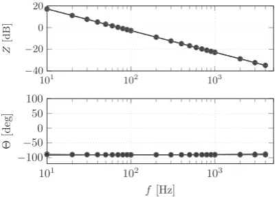
The magnitude of the experimental impedance and angle is shown inFig. 13, where the shape of the magnitude is correlated to the predicted by the analytical methods. However, the angle ob-tained with the physical system does not match the analytical angle for low frequency values (i.e.f_<20 Hz). This problem can be related with some noise problems of the measures at the lower operation point employed. But, as can be seen from the experimental response and the analytical methods the main behavior of the angle is with negative values and a correlation has been found with the theory used to obtain the impedance.

5. Conclusions

The stability analysis of the future interconnection of a DC micro-grid and an AC system was developed. The Nyquist criteria with Thevenin equivalent system were realized. This equivalent was selected due to the behavior and control strategies employed by the converters used in the renewable grid. Where the outer loop was based on voltage control, and the converters have capacitors at the output (i.e. the voltage through them cannot vary suddenly).

As is seen inFig. 9using a low restrictive margin criteria, this analysis predicts the stability at the moment of coupling the AC system with the DC grid. Also, the small disturbances had been consider.

The impedance representation methods used and the stability study can be used with the passivefilter design to improve the quality of the micro-grids.

Appendix A. Parameters of the numerator for the transfer function method

The parameters of the numerator in(17)are presented below, the functionGis¼kpþki/sdescribes the controller in the Laplace domain.

a4 ¼i L_dc 2 (A.1)

a3 ¼KtransG_{a is refd dc}þKtransGaai_{refd is}

2 2

2 2 2_{G i Lv} 2 _{G L2}

a

KtransGaai

2KtransG_{a sd is refd dc dc}

2

E G i Lv þ2i L refdEsdL2

þ2idc aE2sdLvdc

(A.2)

rLþKtransG

a2 ¼ 2KtransG_a2 _{sd is refd dc dc} 2 2 _{dc dc}

2

E G

a

i Lv þi L

a

þ4i rL

a

þi r2

2KtransG_{a sd is refd dc}

2 2 2

E G i rv KtransGaa2irefdEsdL2

þKtransG_{a sd dc}þ2KtransGaai_{refd is}

2 2 2

E rv G rL

þKtransG_{a is refd dc}2KtransGaai

2

G i rv refdEsdrL

þ2KtransG_{a sd dc}

_a

(A.3)

E2Lv

a1 ¼KtransGaai2refdG ris 2þ2i rdc 2

a

2KtransGa2E Gsd isairefdrvdc

2KtransGaa2i_refdEsdrLv_dc2KtransG G i_a3 _is2_refdw L2 2a

þv_dc2 3_aE w L_sd 2 2

a

i_refdþ2i rL_dc

a2

2 2 2 2

KtransG

þKtransG_{a sd dc} þ2KtransG_{a sd} dca

KtransGaai

E Lv

a

E2rv

r2 refdEsd

(A.4)

a0 ¼KtransG_a2 2E r_sd v_dc

a

2þv2_dcKtransG3_{a sd}E ðwLÞ2a2i_refdþi_dcr2

a2

KtransGaa2i_refdEsdr2v_dc

(A.5)

Appendix B. Parameters of the converters

The parameters for the experimental and simulated VSC con-verter with current control are: the AC voltage Es ¼ 200 V,

[image:7.595.79.256.64.154.2]

r¼0.037

U

,L¼3 mH,C¼2.2 mF, the current controller parameters are:kp¼13.3262,ki¼2.96104.

[image:7.595.68.270.192.334.2]

Fig. 11. System configuration to obtain the impedance of the VSC.

Fig. 12.Experimental test-bench used to obtain the impedance of the VSC system.

[image:7.595.67.270.576.719.2]

The DCeDC converter has power rate of 5 kW and the param-eters are:L1¼4 mH,Cf1¼0.3 mF, the current controller gains for

3

parallel PI are kp1¼210 ,ki1¼1.0213, the voltage controller

2

gains are 4.1910 , andki2¼3.476.

The wind turbine and photo-voltaic system have been designed to operate at nominal power at 10 m/s of wind speed, and S¼1000 W/m2respectively. The battery storage system is rated at 3 kW and uses a bidirectional DCeDC converter with a capacitor Cb¼0.18 mF, an inductanceLb¼20 mH, the controller gains for the current loop are kpb ¼106.609, kib ¼ 2.368 105, the voltage

3

controller has the gainskpb2¼41.610 , andkib2¼4.626.

References

[1] Kundur P. Power system stability and control. United States of America: McGraw-Hill; 1993.

[2] Liu J, Feng X, Ye Z, Lee FC, Borojevich D. Stability monitoring using voltage perturbation for dc distributed power systems. J Vib Control 2002;8:277e88. [3] Liu J, Feng X, Lee F, Borojevich D. Stability margin monitoring for dc distrib-uted power systems via current/voltage perturbation. In: Applied power electronics conference and exposition, 2001. APEC 2001. Sixteenth annual IEEE, vol. 2; 2001. p. 745e51.

[4] Feng X, Ye Z, Lee FC, Borojevich D. PEBB system stability margin monitoring. J Vib Control 2002;8:261e76.

[5] Danielsen S, Molinas M, Toftevaag T, Fosso OB. Constant power load charac-teristic’s influence on the low-frequency interaction between advanced electrical rail vehicle and railway traction power supply with rotary con-verters. In: Modern electric traction, 2009 2009. p. 1e6.

[6] Areerak K, Bozhko S, Asher G, De Lillo L, Thomas D. Stability study for a hybrid ac-dc more-electric aircraft power system. IEEE Trans Aerospace Electronic Systems 2012;48(1):329e47.http://dx.doi.org/10.1109/TAES.2012.6129639. [7] Areerak K-N, Bozhko S, Asher G, Thomas D. Dq-transformation approach for

modelling and stability analysis of ac-dc power system with controlled PWM rectifier and constant power loads. In: Power electronics and motion control conference, 2008. EPE-PEMC 2008. 13th. 2008. p. 2049e54.http://dx.doi.org/ 10.1109/EPEPEMC.2008.4635567.

[8] Sun J. Small-signal methods for ac distributed power systems-a review. IEEE Trans Power Electron 2009;4(11):2545e54.

[9] Sun J, Karimi KJ. Small-signal input impedance modeling of line-frequency rectifiers. IEEE Trans Aerosp Electron Syst 2008;44(4):1489e97.

[10] Sun J, Chen M. Analysis and mitigation of interactions between PFC converters and the ac source. In: Power electronics and motion control conference, 2004. IPEMC 2004. p. 99e104.

[11] Sun J, Chen M. Low-frequency input impedance modeling of boost single phase PFC converters. IEEE Trans Power Electron 2004;22(4):1402e9. [12] Sun J. AC power electronic systems: stability and power quality. In: Control

and modelling for power electronics, 2008. COMPEL 2008. 11th workshop on 2008. p. 1e10.

[13] Cespedes M, Sun J. Renewable energy systems instability involving grid-parallel inverters. In: Applied power electronics conference and exposition, 2009 2009. p. 1971e7.

[14] Belkhayat M. Stability criteria for ac power systems with regulated loads. Ph.D. thesis. Purdue University; 1997.

[15] Papathanassiou S, Hatziargyriou N, Strunz K. A benchmark low voltage microgrid network. In: CIGRE symposium 2005. p. 1e8.

[16] Girinon S, Baumann C, Piquet H, Roux N. Analytical modeling of the input admittance of an electric drive for stability analysis purposes. Eur Phys J 2009;47(1):1e8.

[17] Harnefors L, Bongiorno M, Lundberg S. Input-admittance calculation and shaping for controlled voltage-source converters. IEEE Transactions on Industrial Electronics 2007;54(6):3323e34. http://dx.doi.org/10.1109/ TIE.2007.904022.

[18] Khalil HK. Nonlinear systems. 2nd ed. United States of America: Prentice Hall; 1996.

[19] Gelb A, Vander Velde WE. Multiple-input describing functions and nonlinear system design. United States of America: McGraw-Hill; 1968.

[20] Mohan N, Undeland TM, Robbins WP. Power electronics, converters, appli-cations, and design. 3rd ed. United States of America: John Willey & Sons; 2003.

[21] Mohan N. First course on power electronics and drives. United States of America: MNPERE; 2003.

[22] Acevedo S, Giraldo E, Trejos E. Evaluation of power extraction to linear gain scheduling controllers in a small wind energy conversion system. In: Elec-tronics, robotics and automotive mechanics conference (CERMA), 2010 2010. p. 557e62.

[23] Leonhard W. Control of electrical drives. 3rd ed. United States of America: Springer; 2001.

[24] Liu X, Wang P, Loh PC. A hybrid ac/dc microgrid and its coordination control. in press. IEEE Transactions on Smart Grid 2011:1e9. http://dx.doi.org/ 10.1109/TSG.2011.2116162.

[25] Barote L, Marinescu C. Renewable hybrid system with battery storage for safe loads supply. In: PowerTech, 2011 IEEE Trondheim 2011. p. 1e5.http:// dx.doi.org/10.1109/PTC.2011.6019274.

[26] Tremblay O, Dessaint L-A, Dekkiche A-I. A generic battery model for the dy-namic simulation of hybrid electric vehicles. In: Vehicle power and propulsion conference, 2007. VPPC 2007. IEEE. 2007. p. 284e9.http://dx.doi.org/10.1109/ VPPC.2007.4544139.

[27] Guerrero J, Vasquez J, Matas J, de Vicuna L, Castilla M. Hierarchical control of droop-controlled ac and dc microgrids; a general approach toward stan-dardization. IEEE Transactions on Industrial Electronics 2011;58(1):158e72.