Quench dynamics of a disordered array of dissipative coupled cavities

(1)

rspa.royalsocietypublishing.org

Research

Article submitted to journal

Subject Areas:

Condensed matter physics, quantum

physics

Keywords:

cavity QED, many-body physics,

non-equilibrium physics, disorder

Author for correspondence:

C. Creatore

e-mail: [email protected]

H. E. Türeci

e-mail: [email protected]

Quench dynamics of a

disordered array of dissipative

coupled cavities.

C. Creatore

1

, R. Fazio

2

, J. Keeling

3

and H.

E. Türeci

4

1_{Cavendish Laboratory, University of Cambridge,}

CB3 0HE Cambridge, United Kingdom 2_{NEST, Scuola Normale Superiore and Istituto}

Nanoscienze-CNR, I-56127 Pisa, Italy

3_{Scottish Universities Physics Alliance, School of}

Physics and Astronomy, University of St Andrews,

St Andrews KY16 9SS, United Kingdom

4_{Department of Electrical Engineering, Princeton}

University, Princeton, New Jersey 08544, USA

We investigate the mean-field dynamics of a system of interacting photons in an array of coupled cavities in the presence of dissipation and disorder. We follow the evolution of an initially prepared Fock state, and show how the interplay between dissipation and disorder affects the coherence properties of the cavity emission, and show that these properties can be used as signatures of the many-body phase of the whole array.

1. Introduction

The idea of understanding the behaviour of complex quantum many-body systems using experimentally controllable quantum simulators can be traced back to a pioneering keynote speech given by Richard Feynman in 1982 [1]. After thirty years, quantum simulation is now a thriving field of research [2, 3], driven by the increasing ability to design and fabricate controllable quantum systems, in contexts ranging from superconducting-circuits [4] to ultracold atoms [5] or trapped ions [6]. These systems allow the realisation of archetypal models and the exploration of new physical regimes. An area of recently developing interest has been coupled cavity arrays, lattices of coupled matter-light systems, providing highly tunable but dissipative quantum systems [7,8,9,10,11].

c

(2)

2

rspa.ro

y

alsocietypub

lishing.org

Proc

R

Soc

A

0000000

..

[image:2.595.165.432.218.289.2]

Physical realisations of coupled cavity arrays have been proposed in a variety of systems, such as photonic crystal nanocavities [12], coupled optical waveguides [13], or lattices of superconducting resonators operating in the microwave regime [4,14,15]. While experiments have not yet probed the collective behaviour predicted in large scale arrays, progress towards such realisations is very encouraging. For these different systems, the radiation modes involved range from microwave to optical frequency; we will nonetheless refer to these as coupled “matter-light” systems in the following, taking “light” to refer to the radiation modes.

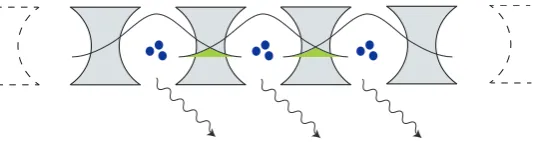
Figure 1.A sketch of a one-dimensional cavity array as described in the text.

A generic coupled cavity array (CCA) consists of a lattice of cavities, each supporting a confined photon quasi-mode. We refer to quasi-modes [16] since the finite quality of the cavities implies there will be coupling to the outside world. As shown in Fig.1, the cavities are coupled through photon hopping. A purely optical system would be entirely linear, and thus unable to simulate interacting many-body quantum systems. To introduce nonlinearity requires coupling to matter (e.g. suitable optical emitters such as semiconductor quantum dots or superconducting qubits, indicated by blue circles in Fig.1). This leads to a system of photons hopping on a lattice, with an on-site nonlinearity and on-site losses.

A wide variety of different microscopic models can be realised depending on the precise design of the array [10,11,15]. We consider here the archetypal case where the CCA can be mapped [10] onto the Bose-Hubbard model [17]. This corresponds to the regime of weak matter-light coupling, i.e. strong detuning between cavity mode and matter degrees of freedom [18].

In the absence of dissipation, the ground state phase diagram of the Bose-Hubbard model has been extensively studied [5]: At zero temperature a quantum phase transition results from the competition between on-site nonlinearities and inter-site photon hopping. When the nonlinearities are strong and prevail over the hopping, the photons are localised by interactions, leading to an insulating Mott phase; in the opposite regime, when photon hopping dominates, a superfluid phase characterised by long-range coherence occurs. Coupled matter-light systems however are naturally studied under non-equilibrium conditions, as there are invariably photon losses. As such, a steady state in a coupled cavity array requires external pumping. The steady-state of cavity arrays, resulting from the competition of external driving and dissipation, has been the subject of much recent theoretical interest [18,19,20,21,22,23].

(3)

3

rspa.ro

y

alsocietypub

lishing.org

Proc

R

Soc

A

0000000

..

Remarkably, even in the lossy system, the dynamics following such a quench clearly map out a superfluid–insulator transition [26]. In fact, in mean-field theory these can be directly related to the equilibrium phase boundary [26,32]. In particular, by rescaling correlation functions by the decaying density one finds that the behaviour at long times is distinct for values of hopping in the superfluid and insulating phases — the rescaled coherence vanishes in the insulating phase, but attains a non-zero asymptote in the superfluid phase. As discussed further below, this can be traced back to the way in which for the closed system quench, the linear stability of an initial Mott state reproduces the equilibrium phase diagram [33]. Given the notable ability of the rescaled correlations of the open system to reproduce the equilibrium phase boundary, and the significant interest in the disordered Bose-Hubbard model [17,34,35,36], a natural question to ask is how the open system quench dynamics are affected by disorder. This is the question we begin to address in this paper. Building on the results of Tomadin et al. [26], we analyse the non-equilibrium mean-field dynamics of an array of non-linear coupled cavities in presence of photon leakage and disorder in the on-site cavity energies.

The paper is organised as follows: In Section 2 we introduce the model used to describe the dissipative and disordered cavity array; in Section 3 we analyse the dynamics of the correlation functions of the cavity array, first summarising the results for the ideal clean case and then assuming a Gaussian distribution for the on-site cavity energies, and compare the results; in Section 4 we briefly discuss an anomalous behaviour of the second order correlation function in presence of disorder; in Section 5 we summarise our conclusions.

2. Model system and initial state

As discussed above, we consider the Bose-Hubbard model [17] described by the Hamiltonian:

ˆ

H=X

i

U

2ˆni(ˆni−1) +εinˆi−J

X

hi ji ˆ

b†_iˆbj. (2.1)

Hereˆb†_i(ˆbi) creates (annihilates) a photon in thei-th site and the corresponding number operator

isnˆi= ˆb†iˆbi. The energy of the photon mode in theith cavity isεi,Jdenotes the amplitude for

inter-site photon hopping, whileUrepresents the on-site nonlinearity resulting from the coupling to matter. Including also the presence of Markovian photon loss leads to the master equation:

∂tρ(t) =−i[ ˆH, ρ(t)] +κ

X

i

D[ˆbi, ρ], (2.2)

where loss is described by the Lindblad termD[X, ρ] = 2XρX†−X†Xρ−ρX†X. The photon lifetime is(2κ)−1. We consider the case whereU, κ, J are independent of site, but there may be disorder in the energiesεi. We will discuss below the “clean” case in which allεiare the same,

and the disordered case where we will choose cavity energies εi to be drawn from Gaussian

distribution having mean value ε¯=ε0 and variance σ2, withσ representing the strength of the disorder. The mean valueε¯can be removed by a gauge transformation, and so may be set to zero without loss of generality. The numerical integration of the master equation has been implemented using a fourth- and fifth-order Runge-Kutta algorithm and we truncate the Fock basis for each cavity to{|nii}nnmax=0withnmax= 4.

We explore the quench dynamics of this model in the mean-field approximationρ=Q

iρi,

(4)

4

rspa.ro

y

alsocietypub

lishing.org

Proc

R

Soc

A

0000000

..

cavity is governed by the master equation

∂tρi(t) =Lρi(t), (2.3)

L=−ihˆhi, ρi(t)

i

+κD[ˆbi, ρi(t)], (2.4)

ˆ

hi=

U

2nˆi(ˆni−1) +εinˆi−J(φi(t)ˆb †

i +φ

∗

i(t)ˆbi), (2.5)

whereφi(t) =Pj∈nn(i)Tr[ˆbjρj(t)]is summed over theznearest neighbours of sitei. In the clean

case all sites are equivalent and soφi(t) =zTr[ˆbiρi(t)], and the dimensionality only enters via this

factorz. In the disordered case, each site evolves separately, and the connectivity of the lattice does affect the dynamics.

Our goal in the following discussion is to study the non-equilibrium dynamics following preparation of the cavity array in a product of Fock states, i.e.ρ(0) =Q

iρi(0), ρi(0) =|n0ihn0|. Because Tr[ˆbiρi(0)] = 0is a fixed point of the mean field equations, we consider a small deviation

away from such a Fock state, and instead considerρi(0) =|Ψ0ihΨ0|, where|Ψ0i=

p

1−η2_|_n 0i+

η|n0−1i. As discussed below, depending on the parameters, the Fock state may be either a stable or unstable fixed point, and if unstable, a small initial perturbationη1will grow, and drive the array to a different asymptotic state.

3. Dynamics of correlation functions

(a) Clean case

Before exploring the role played by disorder, we first summarise the results of the clean case [26] and present also a discussion of the initial instability, first considered in [32] and here thoroughly discussed. In the absence of dissipation, it was shown [33] that whenzJ/U > zJ/U|cr,

wherezJ/U|cris the critical value corresponding to the equilibrium superfluid–insulator phase

transition, an initial Fock state is linearly unstable. As such, the existence of this instability can be used to trace the equilibrium transition between the Mott and the superfluid phase [32,33] and, within our mean-field analysis, a transition survives also in the presence of dissipation.

To see this instability for the clean case, one may write coupled equations for

ρn0−1,n0, ρn0,n0+1 (where n0 is the occupation of the initial state, under the approximation

ρn0,n0'1, and that all other elements ofρare negligible. DenotingX= (ρn0−1,n0, ρn0,n0+1)

T

, one finds that X obeys the equation∂tX=M Xwith

M= iU(n0−1) +izJ n0−κ(2n0−1) (izJ+ 2κ)

p

n0(n0+ 1) −izJp

n0(n0+ 1) iU n0−izJ(n0+ 1)−κ(2n0+ 1)

!

. (3.1)

Instability occurs when the real part of the eigenvalues ofMbecome positive, as this corresponds to exponential growth of fluctuations. In the absence of dissipation (κ= 0), the eigenvaluesξare given by:

ξ=iU

n0− 1 2

−izJ

2 ±i

q

4n0zJ U−(U−zJ)2 (3.2)

The stability boundary is at the point where the eigenvalues are both pure imaginary, and writing

ξ=iµ, one may show that Det(iµ1−M) = 0is equivalent to: 1

zJ=

n0

µ−U(n0−1)

− n0+ 1

µ−U n0 (3.3)

which is the equilibrium phase boundary for the n0th Mott lobe. AszJ increases, the critical values of µin the equilibrium phase boundary approach each other, and at large enoughzJ, there is no longer any real valueµthat can satisfy the above equation. As such, the instability of the Fock state corresponds to the locations of the tips of the equilibrium Mott lobes, zJ/U|_cr= (√n0+ 1−

√

(5)

5

rspa.ro

y

alsocietypub

lishing.org

Proc

R

Soc

A

0000000

..

1

zJ=

−iα2n0

ξ+iU(n0−1) +i(α

2₋

β2)(n0+ 1)

ξ+iU n0

+ iβ 2

(n0+ 2)

ξ+iU(n0+ 1)

. (3.4)

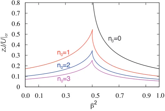
We note that the ground state for any incommensurate filling would always be a superfluid phase. As such, in the equilibrium phase diagram, the critical hopping jumps discontinuously as one varies the filling. Equation (3.4) describes a different question however; namely whether the critical hopping for alinearinstability of the normal state evolves continuously. This is answered by Fig.2, showing that the critical hopping zJ/U|_crfor this instability [obtained solving Eq. (3.4) for differentn0] does evolve continuously as a function ofβ2. In the remainder of this manuscript we restrict to the caseβ= 0.

0.1

0.3

0.5

0.7

0.9 β

2

0

0.1

0.2

0.3

0.4

0.5

0.6

0.7

0.8 zJ/U

cr

0.0

1.0 n =0

n =1

0

n =2

₀

[image:5.595.164.432.288.468.2]

n =3

₀

Figure 2. zJ/U|_cras a function ofβ2_{, the initial state being the statistical admixture}_ρ_{(0) =}_α2_|n0ihn0|₊_β2_|n0₊

1ihn0+ 1|, withα2₊_β2_{= 1}_.

The consequence of this instability can be seen in the time evolution of the coherenceψ(t) = Tr[ˆbiρi(t)]. Figure3shows the evolution ofψi(t)for a clean system withzJ/U > zJ/U|_cr. The

figure is plotted for parametersκ= 10−2U andzJ= 3U, with an initial state withn0= 1, η= 10−5 — we consider this same initial state throughout the remainder of the manuscript. In the initial time range tκ. 0.1, due to the instability, ψ(t) grows exponentially even though the photon populationn(t) =Tr[ˆniρi(t)]decays exponentiallyn(t) =n(0)e−2κ t, see the bottom

inset in left main panel of Fig3. This exponential growth leads to a regime beyond the validity of linearisation, which features underdamped relaxation oscillations ofψ(t). Note that for the conservative caseκ= 0this is replaced by undamped periodic oscillations [33]. At longer times,

tκ >1, the oscillations are damped out but the amplitudeψ(t)also decays to zero asexp(−κt) due to the photon loss. However, the field rescaled by the occupation,ψ¯i(t) =ψi(t)/√ni(t)does

(6)

6 rspa.ro y alsocietypub lishing.org Proc R Soc A 0000000 .. .. .. .. .. .. .. .. .. .. .. .. .. .. .. .. .. .. .. .. .. .. .. .. .. .. .. .. ..

0 0.5 1 1.5 2

0 0.05 0.1 0.15 0.2 0.25 0.3 0.35 0.4 0.45 tκ | ψ ( t ) | 0 0.1 0.2 0.3 0.4 0.5 tκ | ψ ( t ) | / p n ( t )

0 0.5 1 1.5 2 0 0.2 0.4 0.6 0.8 1 tκ n ( t )

0 0.5 1 1.5 2

[image:6.595.117.497.119.249.2]

0 0.2 0.4 0.6 0.8 1 1.2 1.4 1.6 tκ g2 ( t )

Figure 3.Dynamics of a one-dimensional array (z= 2) ofN= 10coupled cavities in presence of a weak dissipation κ= 10−2_U_{and for}_zJ_{= 3}_{U. Left panel: Time evolution of the absolute value of the order parameter}_|ψ₍_t₎_{|. For the} same parameters of the main panel, the bottom inset shows the evolution of the average fillinghni=n(t), while the top inset shows the rescaled order parameterψ(t) =|ψ(t)|/pn(t). Right panel: Time evolution of the zero-time delay second order correlation functiong2(t).

Again, because this quantity is normalized it asymptotically approaches a constant non-zero value (unlessn0= 1). One may in fact show that ifJ= 0,g2(t) =g2(0) = 1−1/n0remains fixed at the value determined by the initial Fock state.

0.1 0.2 0.3 0.4 0.5 0.6 0.7 0.8 0.9

0 0.02 0.04 0.06 0.08 0.1 0.12 0.14 0.16 zJ/U h| ψ ( t )

|it κ= 0.02U

κ= 0.01U

κ= 0.005U

κ= 0.002U

κ= 0.001U

0.10 0.2 0.3 0.4 0.5 0.6 0.7 0.8 0.9

0.2 0.4 0.6 0.8 1 1.2 1.4 zJ/U h g2 it

κ= 0.02U

κ= 0.01U

κ= 0.005U

κ= 0.002U

κ= 0.001U

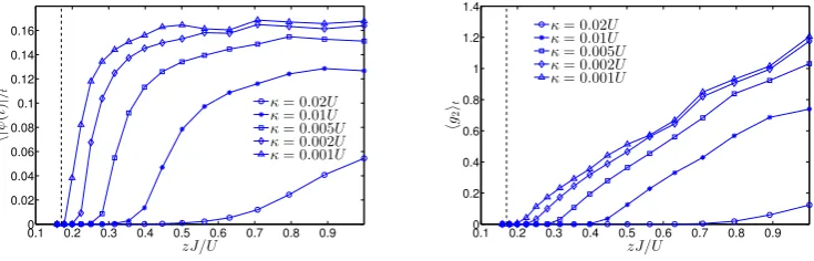
Figure 4.Time average of|ψ(t)|(left panel) andg2(t)(right panel) in the time interval1< tκ <2as a function of the hopping amplitudeJ/Uforκ= 0.001U(triangles),κ= 0.002U(diamonds),κ= 0.005U(squares),κ= 0.01U (asterisks) andκ= 0.02U(circles). The vertical dashed line denotes the value at which the Mott insulator–superfluid transition occurs in the equilibrium Bose-Hubbard model at integer fillingn0= 1,zJ/U|cr≈0.17.

Since the rescaled fieldψ¯(t)and correlation functiong2(t)approach asymptotic values at late times, the behaviour for a given set of initial conditions can be characterised by these values. Formally these are extracted by finding the time-averaged valuesh|ψ|it, hg2it, averaging over

a time window that neglects the initial transients as proposed by Tomadin et al.[26]. Such an approach is illustrated in Figure4, which shows the time-averagedh|ψ|itandhg2itin the time

interval1< tκ <2, as a function of the hopping amplitudeJ/Uand for three different values of the photon decay rateκ. One may clearly see that below a threshold value ofzJ/Ubothh|ψ|itand

hg2itvanish. Asκ→0this threshold approaches the equilibrium superfluid–insulator transition

[image:6.595.120.488.415.533.2]

(7)

7

rspa.ro

y

alsocietypub

lishing.org

Proc

R

Soc

A

0000000

..

(b) Disordered case

We now explore the role played by the on-site cavity disorderεiin the non-equilibrium dynamics.

As discussed above, we thus solve the Liouville problem Eq. (2.3) drawing the cavity energiesεi

from a Gaussian distribution with standard deviationσ. In order to characterise the properties of the ensemble, rather than those specific to a particular realisation, we average the expectations |ψ|andg2over different realisations of disorder, and additionally average over all sites within a given realisation.

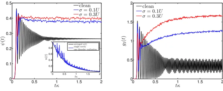
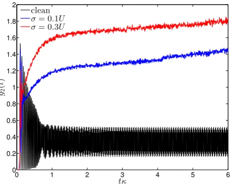
Figure5shows the time evolution of both the order parameter (left panel) and the second-order correlation function (right panel) for a 1D array consisting ofN= 48cavities, averaged over10 realisations of the energies. Except for the distribution of site energiesεi, all other parameters are

as in Fig.3. The site energies are drawn from Gaussian distributions withσ= 0.1U(blue line) and 0.3U(red line). At short timestκ <0.1, the dynamics is characterised by the same linear instability as is seen in the clean case (black line), and bothψ(t)andg2(t)increase exponentially. At later times however disorder strongly modifies the behaviour. The oscillations seen previously in the clean case are washed out by averaging over different cavities, and so a quasi-steady state value is reached earlier.

0 0.5 1 1.5 2

0 0.1 0.2 0.3 0.4 0.5

tκ

ψ

(

t

)

0 0.5 1 1.5 2

0 0.2 0.4 0.6 0.8 1

tκ

n

(

t

)

averagedn(t)

single cavity one disorder realization

clean

σ= 0.₁U

σ= 0.₃U

0 0.5 1 1.5 2

tκ

g2

(

t

)

clean

σ= 0.1U

[image:7.595.116.487.332.484.2]

σ= 0.3U

Figure 5.Dynamics of a disordered one-dimensional array (z= 2) consisting ofN= 48coupled cavities in presence of a dissipationκ= 10−2_U_{and for}_zJ_{= 3}_{U. The simulation has been performed for 10 different realisations of Gaussian} distributed cavity energies withσ= 0.1U(blue line) andσ= 0.3U(red line) Left panel: Time evolution of the absolute value of the order parameter|ψ(t)|. The inset shows the evolution of the average fillinghni=n(t)for a single cavity and a single realisation of disorder withσ= 0.1U(blue line) and after averaging over all the cavities and all the realisations (black line). Right panel: Time evolution of the zero-time delay second order correlation functiong2(t).

As in the clean case, the appearance of a plateau at late times suggests it is possible to characterise the evolution by its asymptotic value (see however the discussion in section 4). Figure6shows the time-integrated|ψ|(left panel) andg2(right panel) as the ratioJ/Uis varied at a fixed photon dissipation constantκ= 10−2Uand for increasing values of disorder strength. As in the clean case, a threshold value ofzJ/Uis required before the instability occurs. This threshold value ofzJ/U for the instability of theψ= 0state appears to increase with increasing disorder. In equilibrium there is a “Bose glass” phase between the Mott insulator and the superfluid [17], where particles are no longer localised by interactions, but are instead localised by disorder. The critical hoppingzJ/U for the equilibrium transition between the Bose glass and superfluid phase increases with hopping, and so our observation of increasing criticalzJ/U. The increasing critical

(8)

8

rspa.ro

y

alsocietypub

lishing.org

Proc

R

Soc

A

0000000

..

0.1 0.2 0.3 0.4 0.5 0.6 0.7 0.8 0.9 1

0 0.02 0.04 0.06 0.08 0.1 0.12 0.14

zJ/U

h|

ψ

(

t

)

|it

clean

σ= 0.1U σ= 0.3U σ= 0.5U σ= 0.7U σ= 0.9U

0.1 0.2 0.3 0.4 0.5 0.6 0.7 0.8 0.9 1

0 0.1 0.2 0.3 0.4 0.5 0.6 0.7 0.8 0.9 1

zJ/U

h

g2

(

t

)

it

clean

σ= 0.1U

σ= 0.3U

σ= 0.5U

σ= 0.7U

[image:8.595.118.498.120.258.2]

σ_{= 0}_.₉_U

Figure 6.Time average of|ψ(t)|(left panel) andg2(t)(right panel) in the time interval1< tκ <2as a function of the hopping amplitudeJ/Ufor fixed decayκ= 0.01Uand increasing disorder strengthσ. The vertical dashed line identifies the value at which the Mott insulator–superfluid transition occurs in the equilibrium Bose-Hubbard model at integer filling

n0= 1,zJ/U|cr≈0.17. Note that, as discussed below, although initial transient behaviour has decayed bytκ=1, the value ofg2continues to evolve, so the right hand panel cannot be interpreted as a steady state.

0 1 2 3 4 5 6

0 0.2 0.4 0.6 0.8 1 1.2 1.4 1.6 1.8 2

tκ

g2

(

t

)

clean

σ= 0.1U

σ= 0.3U

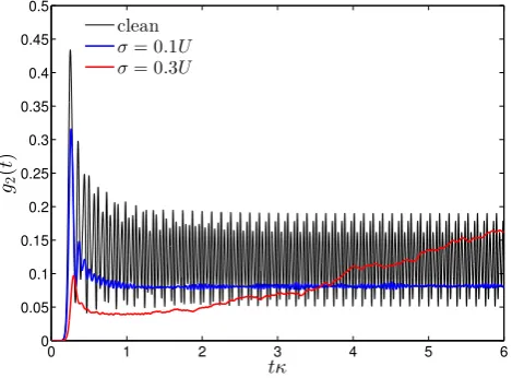
Figure 7.Dynamics of a disordered one-dimensional array (z= 2) consisting ofN= 48coupled cavities in presence of a dissipationκ= 10−2_U_{and for}_zJ_{= 3}_U_{The simulation has been performed for 10 different realisations of Gaussian} distributed cavity energies withσ= 0.1U(blue line) andσ= 0.3U(red line).

4. Rare site statistics at late times

While in the clean case, the plateau reached byψ¯(t)andg2(t)aroundtκ'2reflects the asymptotic time dependence, this turns out not to be the case for the disordered lattice. Despite the appearance of an apparent plateau seen in figure5, this only indicates a temporary plateau. At later times, the values ofhg2(t)idisstarts to rise further as shown in figure7. Intriguingly, this rise

ofhg2(t)idisat late times in fact reflects the existence of rare sites with large and exceptionally

[image:8.595.182.410.376.559.2]

(9)

9

rspa.ro

y

alsocietypub

lishing.org

Proc

R

Soc

A

0000000

..

0 0.5 1 1.5 2 2.5 3 3.5 4 4.5 0

0.1 0.2 0.3 0.4 0.5 0.6 0.7

g2 Pg

2

tκ= 1,σ= 0.3U

0 1 2 3 4 5

0 0.1 0.2 0.3 0.4 0.5 0.6 0.7

Pg

2

g2

5 6 7 8 9 10

0 2 4

x 10−3

g2

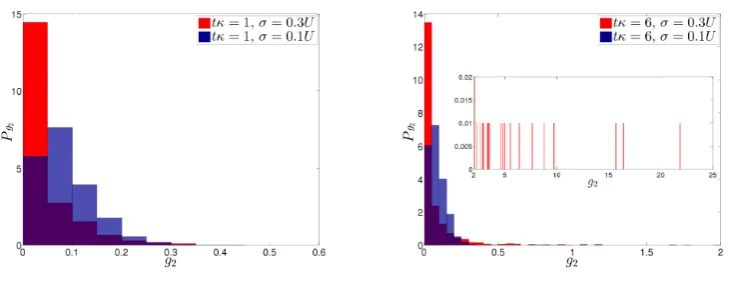
[image:9.595.122.495.119.259.2]

tκ= 6,σ= 0.3U

Figure 8.Probability density ofg2calculated for a 1D array usingκ= 0.01U,zJ= 3Uandσ= 0.3U(see the red curve in Fig.7). The probability density has been evaluated using a sample of 2000 cavities, obtained simulating 20 different

disorder realisations of an array consisting of 100 cavities. Left panel: the probability density ofg2attκ= 1; Right panel: the probability density ofg2attκ= 6. The inset shows the occurrence of rare cavities with values ofg2larger than 5.

0 1 2 3 4 5 6

0 0.05 0.1 0.15 0.2 0.25 0.3 0.35 0.4 0.45 0.5

tκ

g2

(

t

)

clean

σ= 0.1U

σ= 0.3U

Figure 9.Dynamics of a disordered one-dimensional array (z= 2) consisting ofN= 48coupled cavities in presence of a dissipationκ= 10−2_U_{and for}_zJ_{= 0}_.₅_U_{The simulation has been performed for 10 different realisations of Gaussian} distributed cavity energies withσ= 0.1U(blue line) andσ= 0.3U(red line).

used in figure 7 using a sample of 2000 values ofg2, generated after the simulation of a 1D array of 100 cavities for 20 different realisations of disorder withσ= 0.3U (see the red curve in figure7). The right panel shows that, at late times (tκ= 6) some sites exhibit large values (>5) of

g2. The presence of these large values ofg2are the reason thathg2(t)idiscontinues to evolve, and

thus why the right panel of figure6does not indicate a steady state. In the clean system,g2has the same value for all sites, as the state is translationally invariant, thus the appearance of these anomalous values ofg2is a consequence of features of the disorder landscape as we discuss next. This behaviour can be better understood by looking at figure9, which illustrates for a smaller hoppingzJ= 0.5U andκ= 0.01U, how the disorder averagehg2(t)idisrises whenσ= 0.3U(see

[image:9.595.175.410.362.535.2]

(10)

10

rspa.ro

y

alsocietypub

lishing.org

Proc

R

Soc

A

0000000

..

[image:10.595.125.490.117.258.2]

..

Figure 10.Probability density ofg2calculated for a 1D array withκ= 0.01UandzJ= 0.5Uas in Fig.9. The probability density has been evaluated using a sample of 2000 cavities, obtained simulating 20 different disorder realisations of an

array consisting of 100 cavities. Left panel: the probability density ofg2attκ= 1forσ= 0.1U(blue) andσ= 0.3U (red); Right panel: the probability density ofg2attκ= 6. The inset shows that whenσ= 0.3Usome cavities exhibit exceptionally large values ofg2up to&20.

the anomalous sites (i.e. withg21) are local minima of the potential (energy landscape), but not all the local minima exhibit such anomalous values ofg2. Further, following the evolution to much later times becomes difficult, as the large ratio between different elements of the density matrix introduces numerical errors.

5. Conclusions

We have studied the time evolution of the disordered open Bose-Hubbard model following an initially prepared Mott state. As for the clean case, a dynamical transition does occur between small and large values of hopping, signalled by the asymptotic behaviour of the rescaled field

¯

ψ(t). We find that in line with the equilibrium expectations, the presence of disorder does increasezJ/U|_cr, i.e. does increase the hopping required for the superfluid instability to develop. However, even within mean-field theory, disorder can produce anomalous long time dynamics, where ensemble averages are dominated by the effect of rare sites.

6. Acknowledgements

We acknowledge financial support from an ICAM-I2CAM postdoctoral fellowship (under the ICAM Branches Cost-Sharing Fund) for the execution of this work. C.C. gratefully acknowledges support from ESF (Intelbiomat Programme), R.F. from IP-SIQS and PRIN (Project 2010LLKJBX), J.K. from EPSRC programme “TOPNES” (EP/I031014/1) and EPSRC grant (EP/G004714/2), and H.E.T. from NSF CAREER (DMR-1151810) and The Eric and Wendy Schmidt Transformative Technology Fund. We acknowledge helpful discussions with Peter Littlewood.

References

1 Feynman, R. P. 1982 Simulating physics with computers.Int. J. Theor. Phys.,2, 527–556. 2 Jané, E., Vidal, G., Dür, W., Zoller, P. & Cirac, J. I. 2003 Simulation of quantum dynamics with

quantum optical systems. Quantum Inf. and Comp.,3, 15–37.

3 Buluta, I. & Nori, F. 2009 Quantum simulators. Science, 326(5949), 108–111. (doi:

(11)

11

rspa.ro

y

alsocietypub

lishing.org

Proc

R

Soc

A

0000000

..

4 Houck, A. A., Türeci, H. E. & Koch, J. 2012 On-chip quantum simulation with superconducting circuits. Nature Physics,8(4), 292–299. (doi:10.1038/nphys2251)

5 Bloch, I., Dalibard, J. & Zwerger, W. 2008 Many-body physics with ultracold gases. Rev. Mod. Phys.,80, 885–964. (doi:10.1103/RevModPhys.80.885)

6 Monroe, C. & Kim, J. 2013 Scaling the ion trap quantum processor.Science,339, 1064.

7 Hartmann, M. J., Brandão, F. G. S. L. & Plenio, M. B. 2006 Strongly interacting polaritons in coupled arrays of cavities. Nature Physics,2(12), 849–855. (doi:10.1038/nphys462)

8 Greentree, A. D., Tahan, C., Cole, J. H. & Hollenberg, L. C. L. 2006 Quantum phase transitions of light.Nature Physics,2(12), 856–861. (doi:10.1038/nphys466)

9 Angelakis, D., Santos, M. & Bose, S. 2007 Photon-blockade-induced Mott transitions and XY spin models in coupled cavity arrays. Phys. Rev. A, 76(3), 031 805. (doi:

10.1103/PhysRevA.76.031805)

10 Hartmann, M., Brandão, F. & Plenio, M. 2008 Quantum many-body phenomena in coupled cavity arrays.Laser & Photonics Reviews,2(6), 527–556. (doi:10.1002/lpor.200810046)

11 Tomadin, A. & Fazio, R. 2010 Many-body phenomena in QED-cavity arrays [invited]. Journal of the Optical Society of America B,27(6), A130–A136. (doi:10.1364/JOSAB.27.00A130)

12 Majumdar, A., Rundquist, A., Bajcsy, M., Dasika, V. D., Bank, S. R. & Vukovic, J. 2012 Design and analysis of photonic crystal coupled cavity arrays for quantum simulation. Phys. Rev. B, 86(19), 195 312. (doi:10.1103/PhysRevB.86.195312)

13 Lepert, G., Hinds, E. A., Rogers, H. L., Gates, J. C. & Smith, P. G. R. 2013 Elementary array of Fabry-Pérot waveguide resonators with tunable coupling. Appl. Phys. Lett.,103(11), 111112.

(doi:10.1063/1.4820915)

14 Underwood, D. L., Shanks, W. E., Koch, J. & Houck, A. A. 2012 Low-disorder microwave cavity lattices for quantum simulation with photons. Phys. Rev. A, 86(2), 023 837. (doi:

10.1103/PhysRevA.86.023837)

15 Schmidt, S. & Koch, J. 2013 Circuit QED lattices: Towards quantum simulation with superconducting circuits.Annalen der Physik,525(6), 395–412. (doi:10.1002/andp.201200261) 16 Scully, M. O. & Zubairy, M. S. 1997Quantum Optics. Cambridge: Cambridge University Press. 17 Fisher, M. P. A., Weichman, P. B., Grinstein, G. & Fisher, D. S. 1989 Boson localization and the

superfluid-insulator transition.Phys. Rev. B,40(1), 546–570. (doi:10.1103/PhysRevB.40.546) 18 Grujic, T., Clark, S. R., Jaksch, D. & Angelakis, D. G. 2012 Non-equilibrium many-body effects

in driven nonlinear resonator arrays.New Journal of Physics,14(10), 103 025. (

doi:10.1088/1367-2630/14/10/103025)

19 Carusotto, I., Gerace, D., Tureci, H. E., De Liberato, S., Ciuti, C. & ˙Imamo ˘glu, A. 2009 Fermionized photons in an array of driven dissipative nonlinear cavities. Phys. Rev. Lett., 103(3), 033 601. (doi:10.1103/PhysRevLett.103.033601)

20 Hartmann, M. J. 2010 Polariton crystallization in driven arrays of lossy nonlinear resonators. Phys. Rev. Lett.,104(11), 113 601. (doi:10.1103/PhysRevLett.104.113601)

21 Nissen, F., Schmidt, S., Biondi, M., Blatter, G., Türeci, H. E. & Keeling, J. 2012 Nonequilibrium dynamics of coupled qubit-cavity arrays. Phys. Rev. Lett., 108(23), 233 603. (doi:

10.1103/PhysRevLett.108.233603)

22 Jin, J., Rossini, D., Fazio, R., Leib, M. & Hartmann, M. J. 2013 Photon solid phases in driven arrays of nonlinearly coupled cavities. Phys. Rev. Lett., 110(16), 163 605. (doi:

10.1103/PhysRevLett.110.163605)

23 Kulaitis, G., Krüger, F., Nissen, F. & Keeling, J. 2013 Disordered driven coupled cavity arrays: Nonequilibrium stochastic mean-field theory. Phys. Rev. A, 87(1), 013 840. (doi:

10.1103/PhysRevA.87.013840)

24 Werschnik, J. & Gross, E. K. U. 2007 Quantum optimal control theory. Journal of Physics B: Atomic, Molecular and Optical Physics,40(18), R175. (doi:10.1088/0953-4075/40/18/R01) 25 Brierley, R. T., Creatore, C., Littlewood, P. B. & Eastham, P. R. 2012 Adiabatic state

preparation of interacting two-level systems. Phys. Rev. Lett., 109(4), 043 002. (doi:

10.1103/PhysRevLett.109.043002)

(12)

12

rspa.ro

y

alsocietypub

lishing.org

Proc

R

Soc

A

0000000

..

27 Polkovnikov, A., Sengupta, K., Silva, A. & Vengalattore, M. 2011 Colloquium: Nonequilibrium dynamics of closed interacting quantum systems. Rev. Mod. Phys., 83(3), 863–883. (doi:

10.1103/RevModPhys.83.863)

28 Kollath, C., Lauchli, A. M. & Altman, E. 2007 Quench dynamics and nonequilibrium phase diagram of the Bose-Hubbard model. Phys. Rev. Lett., 98(18), 180 601. (doi:

10.1103/PhysRevLett.98.180601)

29 Sciolla, B. & Biroli, G. 2010 Quantum quenches and off-equilibrium dynamical transition in the infinite-dimensional Bose-Hubbard model. Phys. Rev. Lett., 105(22), 220 401. (doi:

10.1103/PhysRevLett.105.220401)

30 Cheneau, M., Barmettler, P., Poletti, D., Endres, M., Schauï¡ ˘g, P., Fukuhara, T., Gross, C., Bloch, I., Kollath, C.et al.2012 Light-cone-like spreading of correlations in a quantum many-body system.Nature,481(7382), 484–487. (doi:10.1038/nature10748)

31 Cai, Z. & Barthel, T. 2013 Algebraic versus exponential decoherence in dissipative many-particle systems. Physical Review Letters, 111(15), 150 403.

(doi:10.1103/PhysRevLett.111.150403)

32 Tomadin, A. 2009 Dynamical instabilities in quantum many-body systems. Ph.D. thesis, Scuola Normale Superiore, Pisa.

33 Altman, E. & Auerbach, A. 2002 Oscillating superfluidity of bosons in optical lattices. Phys. Rev. Lett.,89(25), 250 404. (doi:10.1103/PhysRevLett.89.250404)

34 Gurarie, V., Pollet, L., Prokof’ev, N. V., Svistunov, B. V. & Troyer, M. 2009 Phase diagram of the disordered Bose-Hubbard model. Phys. Rev. B, 80(21), 214 519. (doi:

10.1103/PhysRevB.80.214519)

35 Bissbort, U., Thomale, R. & Hofstetter, W. 2010 Stochastic mean-field theory: Method and application to the disordered Bose-Hubbard model at finite temperature and speckle disorder. Phys. Rev. A,81(6), 063 643. (doi:10.1103/PhysRevA.81.063643)