Estimating gopher tortoise abundance through design based and model based methods

ESTIMATING GOPHER TORTOISE ABUNDANCE THROUGH DESIGN-BASED AND MODEL-BASED METHODS

Payal Bal

A Thesis Submitted for the Degree of MRes Environmental Biology

at the

University of St. Andrews

2010

Full metadata for this item is available in Research@StAndrews:FullText

at:

https://research-repository.st-andrews.ac.uk/

Please use this identifier to cite or link to this item: http://hdl.handle.net/10023/1636

This item is protected by original copyright

Estimating Gopher tortoise abundance through

Design-based and Model-based Methods

Payal Bal

Student ID: 090010807

MRes Environmental Biology

Supervisor: Dr. Len Thomas

Declaration

I, Payal Bal, attest that this dissertation for submission to the School of Biology, University of St Andrews, is entirely my own work.

Signed:

………

Date:

Estimating Gopher tortoise abundance through

Design-based and Model-based Methods

MRes Thesis: School of Biology, August 2010 (39 p.)

By: Payal Bal (MRes Environmental Biology) Supervisor: Len Thomas

Centre for Research into Ecological and Environmental Modelling (CREEM)

University of St Andrews The Observatory

St Andrews

Scotland, KY16 9LZ

Abstract

Table of Contents

Declaration ……… i

Abstract…… ……….. ii

List of Figures ………. iv

List of Tables ………... v

Introduction Gopher Tortoise ………. 1

Data Description ………. 2

Line Transect Sampling Theory ………. 4

Study Objectives ……… 6

Data Analysis Outline ………. 7

Detection Function Detection Function Modelling: In Theory ………. 8

Detection Function Modelling: In Practice ………... 9

Abundance Estimation: Design-Based Approach Design-Based Approach: In Theory ………... 10

Design-Based Approach: In Practice ………. 12

Ichauway Analysis ……….. 12

Fort Gordon Analysis ……….. 15

Abundance Estimation: Model-Based Approach Model-Based Approach: In Theory ……… 20

Model-Based Approach: In Practice ……….. 21

Ichauway Analysis ………... 21

Fort Gordon Analysis ……….. 26

Discussion ……… 34

Conclusion ………... 39

Acknowledgements ……… 39

References ……… 40

Appendices Detection function models ……….. 43

Generalised Additive Models (Model-Based Analysis)…………..………. 46

List of Figures

Figure 1: Distribution and conservation status of the gopher tortoise in the south-eastern United States

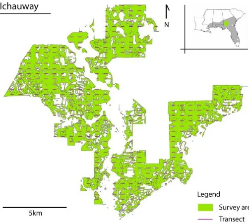
Figure 2: Ichauway location and illustration of the systematic survey design for line transect sampling.

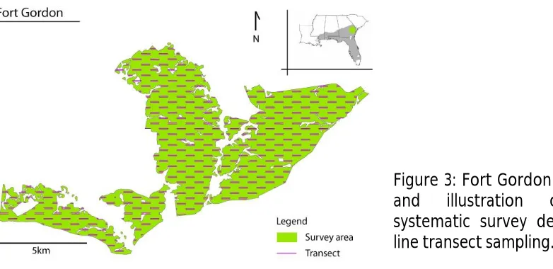
Figure 3: Fort Gordon location and illustration of the systematic survey design for line transect sampling.

Figure 4: Illustrative example of line transect sampling method and analysis Figure 5: (Ichauway) Comparison of encounter rate variance estimators for

systematic design vs. random transect placement

Figure 6: (Fort Gordon) Comparison of encounter rate variance estimators for systematic design vs. random transect placement

Figure 7: (Ichauway) Selected detection function models (Design-based analysis) Figure 8: (Fort Gordon) Selected detection function model (Design-based analysis) Figure 9: (Ichauway) Selected detection function model (Model-based analysis) Figure 10: (Fort Gordon) Selected detection function model (Model-based analysis) Figure 11: (Ichauway) Diagnostic plots for a GAM, modelling burrow abundance

(count data); Surface plot

Figure 12: (Ichauway) Surface plot and variogram for GAM, modelling burrow occupancy (binary data)

Figure 13: (Fort Gordon) Diagnostic plots for a GAM, modelling burrow abundance (count data); Surface plot

Figure 14: (Fort Gordon) Variogram for GAM, modelling burrow occupancy (binary data)

List of Tables

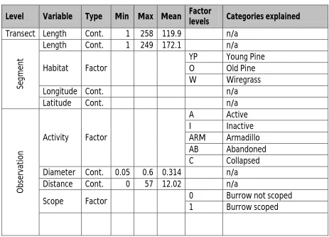
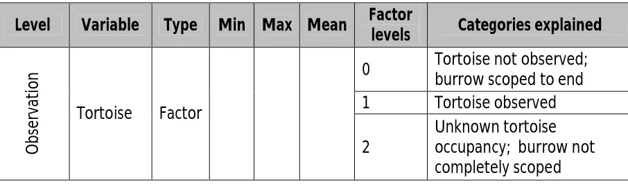
Table I: Summary of Ichauway data

Table II: (Ichauway) Selected detection function models and the associated estimates for design-based analysis using MCDS engine.

Table III: (Ichauway) Stratum-specific density, encounter rate and cluster size estimated from the selected detection function model (DISTANCE results) Table IV: Summary of Fort Gordon data

Table V: (Fort Gordon) Coefficients of the selected detection function model with associated standard errors for Fort Gordon for design-based analysis using MCDS engine

Table VI: (Fort Gordon) Estimates from the selected detection function model Table VII: (Ichauway) Selection of detection function models specified using MRDS

engine

Table VIII: (Ichauway) Summary of selected GAM model with used to predict burrow abundance per segment.

Table IX: (Ichauway) Summary of selected GAM model with used to predict burrow occupancy per segment.

Table X: (Ichauway) Overall and habitat specific abundance point estimates Table XI: (Ichauway) Comparison of variance estimates

Table XII: (Fort Gordon) Selected detection function model for Fort Gordon using MRDS Engine

Table XIII: (Fort Gordon) Summary of selected GAM model used to predict burrow abundance per segment.

Table XIV: (Fort Gordon) Summary of selected GAM model used to predict burrow occupancy per segment.

Introduction

Gopher tortoise

The gopher tortoise, Gopherus polyphemus, is a terrestrial turtle endemic to the United States. It has been under federal or state conservation across its range (Smith et al. 2009) (Fig.1) and continues to be threatened by habitat loss, predation and more recently, by road mortality and respiratory disease (Carthy et al. 2005). Most of the remaining viable populations of the gopher tortoise occur on military installations or private lands where disturbance is minimal (Hermann et al. 2002).

Source: Gopher Tortoise Management Plan, Florida Fish and Wildlife Conservation Commission, September 2007 Figure1: Distribution and conservation status of the gopher tortoise in the south-eastern

United States

The tortoise, 23-28 cm long, spends most of its time in burrows, emerging to feed and look for mates (Ernst & Lovich 2009). Individual tortoises use multiple burrows within a year (Smith et al. 2009). Burrows, characterised by the large a mound of soil or ‘apron’ at the entrance for egg-laying, provide critical habitat for over 300 species of fauna, making the gopher tortoise an ecological engineer and a critical keystone species for longleaf pine habitats.

especially difficult to detect due to the small size of the burrows, as are hatchlings that shelter beneath vegetation rather than excavate burrows (Smith et al. 2009).

Data Description

The data used in this study was collected by the Joseph W. Jones Ecological Research Centre (JWJERC) at Ichauway. Under the Wildlife Population Monitoring Program of the JWJERC, extensive line transect surveys for gopher tortoises were undertaken in two study sites in Georgia, USA, namely Ichauway and Fort Gordon. Surveys included scoping of burrows using a burrow camera scope (Sandpiper Technologies, Manteca, CA) to obtain accurate, rather than subjective, data on burrow occupancy (Carthy et al. 2005).

Study Site: Ichauway

Ichauway is a forest under private ownership, located in south-western Georgia. It is one of the only three protected areas with significant populations of tortoises in Georgia (Smith et al. 2005). The population index derived from the track count surveys suggest that the gopher tortoise population at Ichauway has declined in spite of habitat management (Ichauway Adaptive Management Proposal, Smith et al. 2006). However, no population estimates have been made till date for the tortoises at Ichauway from previous surveys.

Line Transect Data: Systematic surveys were conducted on a 6870 ha study area

during April – September 2006 and April – October 2007. Detectability was assumed constant for the two sampling occasions as the habitat on a whole is consistently open and adult burrows were easily detected regardless of the state of the vegetation during the year. Juvenile burrows were infrequent and much more difficult to find but they were not the population of interest for the estimate (Stober, J., pers. comm.). The study area has three predominant habitat types, young pine (<30 years post plough), Oldfield pine (all mature pine habitat without wiregrass understory), wiregrass (with pine overstory, agriculture or unsuitable). Data collection teams consisted of four people on the field (1 scoping burrows, 2 identifying burrows, and 1 recording data).

419 line transects measuring 250m in length were placed at 400m intervals (east-west and north-south) according to a square grid. The following information was collected during the survey:

● Perpendicular distance to burrows detected from the transect centre line ● Habitat type at burrow location

● If the burrow was scoped

● If a tortoise was observed

● Burrow activity class: active, inactive, abandoned, collapsed or armadillo burrow

● Burrow diameter

Armadillo, abandoned and collapsed burrows were scoped only when occupancy was uncertain. GIS files of study area (including ground cover, land cover, topology maps and management zones) and transect locations were also made available.

Study Site: Fort Gordon

Fort Gordon in eastern Georgia is primarily a communications training centre for the U.S. Army. Its long leaf pine forests and savannas are ideal for the gopher tortoise.

Line Transect Data: Systematic surveys were conducted within a 7246 ha

Figure 3: Fort Gordon location and illustration of the systematic survey design for line transect sampling.

300 pairs of parallel 500m segments that were 50m apart (pseudo-circuit design) were laid according to a triangular grid. The pseudo-circuits were separated by 500 m in the east-west and 300m north-south directions (JWJERC Fort Gordon report, 2010). Information collected (and available for analysis):

● Perpendicular distance to burrows detected from the transect centre line ● If a tortoise was observed

No ancillary information on habitat or burrow characteristics was available for analysis for this dataset. GIS files of study area (including soil maps), transect locations and detections (along with burrow details) were made available.

Line transect sampling theory

Distance sampling includes a number of methods, all of which involve measuring or estimating distance to detected animals or clusters of animals from a line or point of observation (Borchers et al. 2002). Line transect sampling is one such method. The general approach to line transect sampling is detailed below:

1. A survey design with random or a systematic transect placement is overlaid on the study area

2. Perpendicular distances from the centreline to the detected object are recorded. Transect lengths and the distance up to which detections are recorded (truncation distance) define the covered area (sampled area) for the survey

4. The estimated detection probability is used to estimate abundance in the covered area

5. The estimate of the covered area is scaled up to get an estimate of the total abundance of the survey region1.

The key idea in distance sampling is that animals within the covered area may be missed and need to be accounted for when extrapolating the count in the sample to the total number in the area.

Critical considerations for Line transect sampling

Unbiased estimates of density/abundance can be obtained if some critical assumptions are met: (i) probability of detecting an animal on the transect is 1; (ii) animals being counted do not move away or closer to the line in response to the observer; (iii) perpendicular distances to the animals are measured without errors (Buckland et al. 2001).

Line transect data analysis

Estimating abundance from line transect data can be broadly divided into two parts: 1) Detection function modelling and 2) Abundance estimation. Abundance estimation can be done in one of the two following ways:

Design-Based approach: This framework considers animal locations as fixed and

allows for random placement of transects. The approach works under the assumption of equal coverage probability due to which the estimates of abundance and variance are mainly design dependent. Estimators for variance in this framework can vary according to the survey design (Fewster et al. 2009).

Model-based approach: This approach allows for movement of animals among

surveys, while sampling plots remain fixed. Animal locations are drawn from a fixed spatial probability density that is modelled based on available data on animal counts and environmental variables (Fewster et al. 2009). Variance can be estimated by bootstrapping.

1 _{If the object being detected is a cluster rather than an individual, abundance of animals can be calculated}

This thesis is divided into four main sections. The first section details the detection function modelling theory behind abundance estimation. The second section details the design-based approach to abundance estimation. Encounter rate variance estimates for systematic survey design are calculated and compared to the default R2 estimate (suited to random line placement) in DISTANCE 6.o. The third section details the model-based approach for abundance estimation. GAMs for modelling burrow density and burrow occupancy are specified using available environmental covariates. Variance is estimated by means of bootstrapping; both non-parametric and parametric variance estimates are calculated and compared. Finally, the discussion analyzes the design-based and model based results for the two study sites and highlights the weak points of the study. Some improvements for the two approaches are suggested as follow up work to the project

.

Study Objectives

Data Analysis Outline

Design-Based Approach

1. Detection function was modelled as a function of perpendicular distance in CDS and MCDS engine of DISTANCE 6.0 (Thomas et al. 2010). Environmental covariates that could affect detection probability were included to find the best fitting model.

2. The cluster size estimation technique to scale burrow abundance to tortoise abundance was used.

3. Tortoise abundance was estimate by using predicted detection probability, pˆ . 4. Variance of abundance estimate was calculated by the delta method (Buckland et

al. 2001).

5. Encounter rate variance was calculated using alternative estimators to account for systematic survey design (Fewster et al. 2009).

Model-Based approach

1. Detection function was modelled in MRDS engine of DISTANCE 6.0 (Thomas et al. 2010) according to environmental covariates (where relevant).

2. Predicted pˆfrom the selected model was used to calculate effective strip half-width for each segment (i.e. subdivision of the transect).

3. Burrow abundance in the covered area was modelled as a function of environmental covariates using the mgcv package (version 1.6-1) in R 2.9.1.

6. Burrow occupancy in the covered area was modelled as a function of environmental covariates.

7. Using the corresponding model coefficients, burrow abundance and occupancy were predicted for a grid covering the study area. Abundance and occupancy were multiplied to give an estimate of tortoise abundance for each grid cell.

8. The estimates were summed to give a point estimate of abundance for the entire study area.

Detection Function

Detection Function Modelling: In Theory

The detection function is the probability of detecting an animal within the covered area, given its characteristics and other associated environmental or survey-level variables (Borchers et al. 2002). When it is not known, the detection function can merely be treated as a decreasing function with increasing distance from the transect centreline (where detection probability is 1) to a predetermined truncation distance. It allows for the fact that animals further away from the centreline are more difficult to see. By modelling the decrease (solid line in Fig. 4), line transect methods can give estimates of the proportion of animals missed (Borchers et al. 2002) under the assumption that target species is distributed uniformly within the strip.

Source: Marques, T. 2009. ‘Distance Sampling: Estimating animal density’ toolkit. Available at: http://www.ruwpa.st-and.ac.uk/distance.book/toolkit.pdf

Figure 4: Illustrative example of line transect sampling method and analysis

Note on Effective Strip Half-Width ( ): It is the distance from the transect centreline on either side such that as many, objects are detected outside the strip as remain undetected within it (Buckland et al. 2001). Simply put, it gives the effective area covered (A) within which all animals are detected. Mathematically,



pˆ _{Effective area covered/Actual area covered}

w wL

L  

 

2 2

Model Specification: The general form of a detection functiong





 

 











 



where yis the measured/estimated perpendicular distances

zare the covariate value(s)

key represents the key function

series represents the series expansion



/

y

yS  where is the scale parameter of the key function, modelled as

an exponential function of the covariates (Buckland et al. 2001, Harris 2007). The key function is the starting point for detection function modelling while the series expansion gives flexibility to the key function to improve model the fit (Buckland et al. 2001).

Model selection: Detection function models can be compared on the basis of the AIC

(Akaike's Information Criterion) and the shape criterion. The AIC statistic is a measure of fit

of the model which is increasingly penalized with additional parameters estimated from the model (Buckland et al. 2001). A relatively lower AIC score indicate a better fit of the model. Mathematically, AIC 2log_e

 

where log_e

 

According to the ‘shape criterion’ defined by Burnham et al. (1980), a detection function should ideally have a ‘shoulder’, be non-increasing and have a tail that goes asymptotically to zero (Buckland et al. 2001). Quantile-Quantile (Q-Q) plots and hypothesis tests (Kolmogorov-Smirnov and Cramér von Mises) may also aid in model selection.

Detection Function Modelling: In Practice

All models for the design-based approach were run in the CDS and MCDS engine (Thomas et al. 2010) in program DISTANCE (Version 6.0). Models for the model-based approach

Abundance Estimation: Design Based Approach

Design-Based Approach: In Theory

This framework considers animal locations as fixed and allows for random placement of transects. The approach makes the assumption of equal coverage probability i.e. all parts of the survey area have an equal probability of being sampled (Buckland et al. 2001). As a result the estimates of abundance as well as variance are mainly design dependent.

Abundance Estimation: The abundance of the target species for the entire area is

estimated as p wL nA N ˆ 2

ˆ _{ …Eq. 3}

where n is the total number of animals counted within the covered area A is the total area of the survey region

w is the truncation distance L is the total transect length

pˆ is the detection probability (calculated using the detection function)

L n

is also known as the encounter rate.

To estimate density, the abundance estimate (Nˆ ) is merely divided by the total area of the survey region (A).

Variance for Design-Based estimates: Estimators for the design-based framework

can vary according to survey design. Traditionally, variance estimators for random design have been applied even in the case of systematic design. This “discounts for the lower variance achieved by systematic survey designs at the estimation stage” (Fewster et al.

2009).

Overall abundance variance can be estimated using the delta method under the assumption that the correlations between the components are zero (Buckland et al. 2001).

 







 



 

 





 

L n cv N cv s cv p cv n cv N cv 2 2 2 2 2 2 2 2 ˆ ) ˆ ( ˆ ) ˆ (                    …Eq.4

ˆ is the estimated effective strip half-width; and D D ar V D D se cv ˆ ) ˆ ( ˆ ˆ ) ˆ (   …Eq.5

The encounter rate variance usually dominates the overall variance of abundance (Fewster et al. 2009). DISTANCE 6.0 calculates the encounter rate variance according to the R2 estimator of Fewster et al. (2009):







where nand Lare the same as specified above kis the number of transects

i

l is the line length of transect i

Other estimators based on random design, listed in Fewster et al. (2009) include a variant of R2 for constant L (R1) and a model-derived estimator (R3).

















vˆ …Eq.8

Fewster et al. (2009) suggest alternate estimators suited to systematic survey design:













 kh

j n hj h hj H h h h l l L n n n k k L L n S 1 2 1 2 1 1 1 ar vˆ …Eq.9

where His the total number of strata

h

k is the number of transects in stratum h

hj

l is the th

j transect length in stratum h

hj

n is the number of observations on the th

j transect in stratum h

h

n and lhare the within stratum means

The stratum specific variance estimate can be pooled in a heuristic manner, weighting by total line length per stratum to get an alterative estimator for the stratified case (Fewster

et al. 2010): _

           



2 vˆar

1

var …Eq.10

where nhandLhare stratum specific totals

h

h

ar

R1 ignores the variance in L and is not recommended while R3 is only applicable if the model specifying underlying animal locations is accurate. R2 works well in case of random designs. S1 and S2 are known to show a significant improvement over R2 for systematic designs (Fewster et al. 2009) as they capture the spatial correlation between transects in a systematic design (Distance User’s Guide).

Design-Based Approach: In Practice

Ichauway

Data Preparation: 298 out of a total of 419 transects, with complete information

and which lay inside the study area, were used for analysis. Most transects were divided into more than one segment at the time of data collection; each transect was made up 2.5 segments on average. Total transect lengths were calculated by adding up segments lengths under the same transect ID in GIS files. Segment centre coordinates were calculated in ArcGIS (Version 9.3) for mapping burrow locations and to use in analysis as spatial variables.

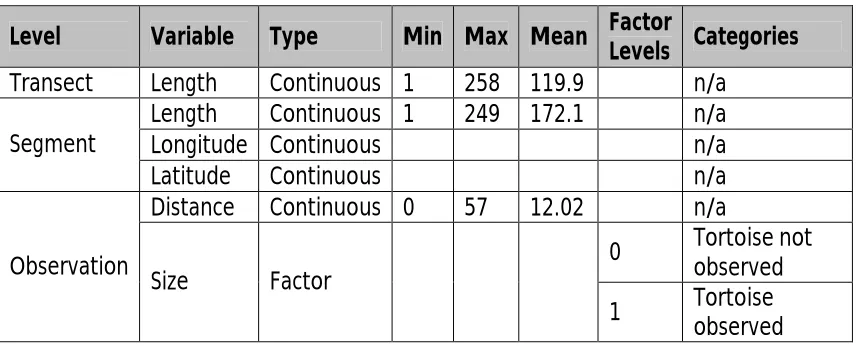
Table I: Summary of Ichauway data

Level Variable Type Min Max Mean Factor

levels Categories explained

Transect Length Cont. 1 258 119.9 n/a

Length Cont. 1 249 172.1 n/a

YP Young Pine

O Old Pine

Habitat Factor

W Wiregrass

Longitude Cont. n/a

Se

gm

en

t

Latitude Cont. n/a

A Active

I Inactive

ARM Armadillo

AB Abandoned

Activity Factor

C Collapsed

Diameter Cont. 0.05 0.6 0.314 n/a

Distance Cont. 0 57 12.02 n/a

0 Burrow not scoped

Scope Factor

1 Burrow scoped

O

b

se

rv

at

io

n

Level Variable Type Min Max Mean Factor

levels Categories explained

0 Tortoise not observed;

burrow scoped to end

1 Tortoise observed

O

b

se

rv

at

io

n

Tortoise Factor

2

Unknown tortoise occupancy; burrow not completely scoped

Detection function model: Data was right truncated at 35m to avoid fitting to

outliers (Buckland et al. 2001). The cluster-size estimation technique was used to estimate the number of occupied burrows and the population estimate based on the number of tortoises observed in burrows (Buckland et al. 2004, JWJERC Fort Gordon report, 2010). The cluster size of occupied burrows was set to 1, whereas for unoccupied burrows the cluster size was 0. Preliminary models were run in CDS engine of DISTANCE 6.0 (Thomas et al. 2010) with and without post-stratification. Post-stratification models outperformed

the former. Proportion of occupied burrows was calculated using mean of observed clusters (JWJERC Fort Gordon report, 2010).

Segment level covariates (habitat, latitude, longitude) were included in the detection function using the MCDS engine in DISTANCE 6.0 (Thomas et al. 2010). Available observation level covariates were not included in the modelling because burrow characteristics (diameter at the mouth) or occupancy (activity) were not expected to affect detection (Nomani et al. 2008). Post-stratification model without covariates and with built in model-selection had the lowest AIC score (Appendix1: Ichauway). Built-in model selection allowed for different detection functions to be specified for each habitat type.

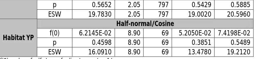
Table II: Selected detection function models and the associated estimates for design based analysis using MCDS engine. (Refer Fig. 7 for selected function plots)

Stratum Estimate %CV df 95% CI

Hazard/Polynomial

f(0) 5.4960E-02 3.77 371 5.1001E-02 5.915E-02

p 0.52020 3.77 371 0.4831 0.5602

Habitat O

ESW 18.2070 3.77 371 16.9070 19.6070

Uniform/Cosine Habitat W

p 0.5652 2.05 797 0.5429 0.5885

ESW 19.7830 2.05 797 19.0020 20.5960

Half-normal/Cosine

f(0) 6.2145E-02 8.90 69 5.2050E-02 7.4198E-02

p 0.4598 8.90 69 0.3851 0.5489

Habitat YP

ESW 16.0910 8.90 69 13.4780 19.2120

f(0) - value of pdf at zero for line transects = 1/u p - Probability of observing an object in defined area ESW - Effective strip width = W*p

Wiregrass habitat appeared to have higher detection probability although all habitats had comparable probabilities overall.

Abundance estimates: The overall density estimate was calculated by taking a

mean of the stratum estimates and weighting them by effort in each stratum. Density was highest for wiregrass habitat (Table III). Stratum specific estimates in turn are calculated according to Eq. 3. Estimated tortoise abundance for Ichauway (6870 ha) was 29015 + 2001 2, indicating high uncertainty associated with the estimate. Overall variance was estimated according to Eq. 4 using the R2 estimator for encounter rate (Eq. 6), which does not account for the systematic survey design. Encounter rate variance was calculated separately for each habitat type.

Table III: Stratum-specific density, encounter rate and cluster size estimated from the selected detection function model (DISTANCE results)

Stratum Estimate %CV df 95% CI

n/L 1.60E-02 7.41 187 1.38E-02 1.85E-02

D 3.3695 12.26 323.45 2.6497 4.2849

Habitat O

S 4.3874 8.31 286.64 3.7262 5.1659

n/L 2.94E-02 6.32 160 2.60E-02 3.33E-02

D 5.7243 8.38 420.79 4.8559 6.748

Habitat W

S 7.4322 6.65 195.05 6.5197 8.4725

n/L 7.74E-03 25.46 72 4.70E-03 1.28E-02

D 1.9242 35.64 75.28 0.96628 3.8317

Habitat YP

S 2.4052 26.97 89.3 1.4207 4.072

Pooled Estimates

D 4.2235 6.9 789.95 3.6889 4.8355

S 5.4744 5.2 416.52 4.9431 6.0627

n/L – Encounter rate

D – Estimate of density of animals

S – Cluster size (in this case burrow occupancy)

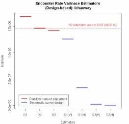
Variance estimation for systematic survey data: Due to the large number of

transects, a non-overlapping post-stratification scheme consisting of pairs of adjacent transects was applied to the data. Estimators based on overlapping strata were not examined. S1 and S2 estimators for horizontal and vertical (1-dimensional) paring were calculated and compared to R1, R2 & R3 estimators (Fig. 5).

Figure 5: Comparison of encounter rate variance estimators for systematic design vs. random transect placement; S (V) and S (H) indicate estimators for vertical and horizontal

pairing of transects, respectively.

As expected, encounter rate variance estimators for systematic design give lower variance compared to estimators for random design. There appears to be a large difference between S1 and S2 estimates for the vertical pairing unlike for the horizontal pairing.

Fort Gordon

Steps involved in analysis were the same as those detailed for Ichauway.

Data Preparation: Pairing of the 500m segments of the pseudo-circuits was done

time of data collection. On average however, each transect was made up of 2 segments. Segment centre coordinates were calculated in ArcGIS (Version 9.3) for use in analysis as spatial variables.

Table IV: Summary of Fort Gordon data

Level Variable Type Min Max Mean Factor

Levels Categories

Transect Length Continuous 1 258 119.9 n/a

Length Continuous 1 249 172.1 n/a

Longitude Continuous n/a

Segment

Latitude Continuous n/a

Distance Continuous 0 57 12.02 n/a

0 Tortoise not

observed Observation

Size Factor

1 Tortoise

observed

Detection function model & Abundance Estimate: Data was truncated at 25m to

avoid overlap between strip half widths of adjacent segments of the pseudo-circuits. Models were run in the CDS engine of DISTANCE 6.0 (Thomas et al. 2010). Segment level covariates (latitude, longitude) were included in the detection function using the MCDS engine in DISTANCE 6.0 (Appendix1: Fort Gordon).

Table V: Coefficients of the selected detection function model with associated standard errors for Fort Gordon for design-based analysis using MCDS engine

Half-normal/Cosine

Covariate Point Estimate Standard Error

Intercept 14.89 1.069

Longitude 0.2283 0.3144

Table VI: Estimates from the selected detection function model for Fort Gordon

Parameter Estimate %CV df 95% CI

f(0) 5.77E-02 6.42 84 5.08E-02 6.55E-02

p 0.69322 6.42 84 0.61026 0.78745

ESW 5.77E-02 6.42 84 5.08E-02 6.55E-02

n/L 3.70E-04 15.34 299 2.74E-04 5.00E-04

D 3.11E-02 23.74 270.28 1.96E-02 4.92E-02

Overall density was estimated as 0.0311 + 0.0074; and tortoise abundance for Fort Gordon (7246 ha) as 225+ 53.6.

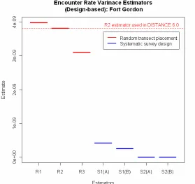
Variance estimation for systematic survey data: Pairing was done diagonally

because of the triangular grid used in the systematic transect layout. S1 and S2 estimators (1-dimensional) were calculated and compared to R1, R2 & R3 estimators (Fig. 6).

Figure 6: Comparison of encounter rate variance estimators for systematic design vs. random transect placement; S (A) and S (B) indicate estimators for the two types of

(1-dimensional) pairing of transects.

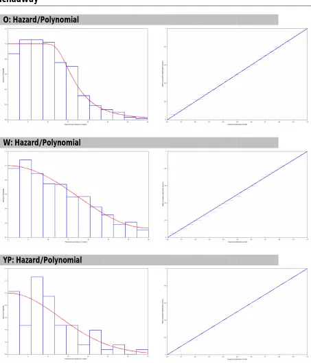
Figures 7-8: Detection Function Model Plots

Ichauway

O: Hazard/Polynomial

W: Hazard/Polynomial

YP: Hazard/Polynomial

Figure 7: (Ichauway) Selected detection function models from the design-based analysis for each habitat type. Corresponding Q-Q plots indicate well fitting models. The fitted

cumulative distribution function (cdf) is plotted in increasing size order against the empirical distribution function (edf). A well fitting model is indicated if points (shown in

Fort Gordon

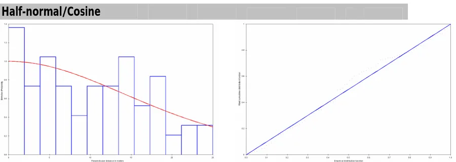
Half-normal/Cosine

Abundance Estimation: Model Based Approach

Model-Based Approach: In Theory

Abundance Estimation: This approach allows for movement of animals among

surveys, while sampling plots remain fixed. Animal locations are drawn from a fixed spatial probability density that is modelled based on available data on animal counts and environmental variables (Fewster et al. 2009). It allows inference regarding animals not seen within the covered area.

The spatial model itself may explain some of the variation in density (in the covered area) by using covariates that may be ecologically meaningful to the target species. However, the model may only act as a predictive tool, as the covariates used may merely be proxies for more important, unknown variables (Buckland et al. 2004, Harris 2007).

Model Specification: Generalized Linear/Additive Models (GLMs or GAMs) may be used to

specify these spatial models. In most cases, GAMs have an advantage over GLMs as they do not follow the linearity assumption of GLMs. GAMs are of the general form:

 



E

y







_

s

 

x

f



where f represents the link function 0

 is the intercept term

 

k x

s is the smooth function f the explanatory variable k

Model Selection: The General Cross Validation (GCV) score for unknown scale parameter

models or the UBRE scores for known scale parameter models, percentage of deviance explained and the adjusted r-sq values are used in model selection for GAMs. Q-Q plots and observed vs. fitted plots assess model fit. Histogram of the residuals can help asses the correct error distribution to be used for the model. Finally, constant variance is indicated by a constant band of residuals when plotted against the linear predictor, i.e. with increasing mean, and can help assess if the correct variance structure has been specified for the model (Wood, 2006).

(Cañadas & Hammond, 2006 in Harris 2007). Cluster size may also be modelled using spatial covariates, if required, and an overall abundance estimate can be given by multiplying the corresponding predictions of cluster size and cluster abundance (Buckland et al. 2004, Harris 2007).

Variance for Model-Based estimates: Variance estimation is done by

bootstrapping. The basic approach is to generate multiple resamples from the original data, of the same size as the data (i.e. with replacement), and produce abundance estimates for each of the resamples. The resulting distribution of the simulated estimates is then used estimate the overall variance (Borchers et al. 2002).

Model-Based Approach: In Practice

Ichauway

Data Preparation: Data used was the same as that for the design-based approach.

Detection function: Data was truncated at 35m to avoid fitting to outliers.

Preliminary models were run in the MRDS engine of DISTANCE 6.0 (Thomas et al. 2010) with segment-level covariates (habitat, latitude, longitude). Observation level covariates (burrow type and diameter) were not included as they were not expected to affect detection (Nomani et al. 2008). No post-stratification or built-in model selection could be specified in the MRDS engine.

Table VII: Selection of detection function models specified using MRDS engine for Ichauway dataset

Model A (lat + long + habitat) Model B (habitat)

Covariates Point Estimate Standard Error Point Estimate Standard Error

Intercept (Habitat 0) 2.5008 0. 04483196 2.50067828 0.04317676

Habitat W 0.2849 0.05793947 0.28198195 0.05545213

Habitat YP -0.0022 0.10547436 0.05839115 0.10370975

Latitude 0.0389 0.03051761

Longitude 0.0600 0.02889826

Half-normal key function models performed better than hazard rate models. Out of the half-normal models, detection function seemed to be best explained by habitat type and spatial location. However the best fit model (Model A) only showed a marginal improvement in AIC score over Model B (Table VIII), and included latitude and longitude as linear terms rather than as a surface. This made interpretation with respect to Model A difficult and hence Model B was selected for further analysis. Furthermore, predictions from the two models were very similar. Average pˆ from the selected model was 0.5102 + 0.01181 (CV = 0.0234).

Effective Strip-Half Width: The selected detection function was used to predict

pˆfor each segment and was multiplied by the truncation distance (35m) to get the effective strip half-width for each segment. The effective area surveyed was calculated by multiplying the effective strip half-width by the length of the corresponding segment.

Abundance estimates: Tortoise abundance was calculated by multiplying model

predictions for burrow abundance and burrow occupancy. Data was truncated at 35m.

1. Burrow Abundance in Covered Area: Generalized additive models (GAMs) using the

mgcv package (version 1.6-1) in R (Version 2.9.2) were fitted to data from all segments. Total number of burrows per segment (count data), n, was calculated to use as the response variable. Poisson with overdispersion (scale fitted from the most complicated model with quasipoisson error distribution) and Negative Binomial error distributions were examined for all the models, with the log link function. Segment-level covariates used for detection function modelling were also used in the GAMs; interactions terms (latitude, longitude) were also included. Continuous covariates were entered as smooth terms with shrinkage to allow smooth terms to be reduced to zero if not significant, thereby making no contribution to the model (Wood, 2006). Overfitting in the model or wiggliness was controlled by the specifying gamma parameter to 1.4 (Wood, 2006)3. The effective degrees of freedom (determining smoothness) were decided automatically by minimizing the GCV scores (Wood, 2006). Effective area surveyed was specified as an offset instead of modelling expected number of observations per segment (calculated

3_{The gamma parameter forced each effective d.f. in the model to be counted as 1.4 d.f. in the GCV, making}

using the Horvitz-Thompson estimator4) and to negate the effect of unequal segment sizes influencing values of n.

AIC was used for model selection among models using negative binomial error distribution instead of UBRE. QAIC was used in case of models with overdispersion (Poisson error distribution models). QAIC scales the deviance used in the AIC equation (Eq.1) by the overdispersion (): QAIC e

 

2 log

2

 



 …Eq. 11

AIC/QAIC scores agreed in general with the model UBRE scores. (Refer Appendix 2: Ichauway for details of fitted models)

Both error distributions selected the same model. The poisson error distribution model was selected over negative binomial as it appeared to have slightly higher predictive power. The final GAM model (to explain burrow abundance in covered area) included latitude and longitude (as a surface) and habitat as explanatory variables (Table VIII, Fig. 11).

Table VIII: (Ichauway) Summary of selected GAM model with used to predict burrow abundance per segment. The model used a poisson error distribution with log link function. Estimated coefficient values (and standard errors) of parameters are displayed, with the results of a z-test. Habitat type O act as a baseline parameter and is included in the intercept.

Parametric coefficients:

Covariates Estimate Std. error z-value Pr(>|z|)

intercept -7.0720 0.0333 -212.44 < 2e-16

Habitat W 0.1493 0.0403 3.70 0.0002

Habitat YP -0.5079 0.0939 -5.41 6.3E-08

Approximate significance of smooth terms:

edf Ref.df Chi.sq p-value

Latitude, Longitude 27.83 28.89 746 < 2e-16

R-sq.(adj) = 0.702

Deviance explained = 40.7% Scale est. = 1.5942

Wiregrass habitat appears to be the most significant predictor of burrow abundance.

4 _{Horvitz-Thompson estimator (Horvitz & Thompson, 1952),}







i n

j ij

i

p N

1 ˆ

1 ˆ

2. Burrow Occupancy in Covered Area: A subset of the total data, with certain burrow

occupancy, was used for the analysis. Data was not truncated. GAMs used for burrow occupancy were specified using presence/absence of tortoise (in the burrow) as a binary response. No offset term was specified. The binomial error distribution with logit, probit and cloglog link functions were tested in the models. UBRE scores were consulted for model selection (Appendix 2: Ichauway).

The cloglog models had the lowest UBRE scores; however these were only marginally different from models with the logit link transformation. Therefore, the simpler model with the logit link was selected for easier interpretation.

Table IX: (Ichauway) Summary of selected GAM model with used to predict burrow occupancy per segment. The model used a binomial error distribution with logit link function. Estimated coefficient values (and standard errors) of parameters are displayed, with the results of a z-test. Habitat type O act as a baseline parameter and is included in the intercept.

Parametric coefficients:

Covariates Estimate Std. error z-value Pr(>|z|)

intercept -2.0351 0.1767 -11.5160 < 2e-16

Habitat W 0.6338 0.2112 3.0020 0.0027

Habitat YP -0.1604 0.4904 -0.3270 0.74354

Approximate significance of smooth terms:

edf Ref.df Chi.sq p-value

Latitude, Longitude 20.07 24.59 49.75 1.94E-03

R-sq.(adj) = 0.0478

Deviance explained = 7.25% Scale est. = 1

High standard error associated with the predictions for this model (i.e. 0.1494 + 2), adjusted R-sq., deviance explained and diagnostic plots (Fig. 12), all indicate a poor model. (Predictions from the model are used for the purpose of illustrating the model-based approach).

3. Tortoise Abundance: Burrow abundance and occupancy were predicted for the entire

abundance for the entire study area. Maps depicting abundance predictions from the above specified models were prepared in ArcGIS (Version 9.3) by natural neighbour interpolation5 (Fig. 15). Predicted tortoise abundance for the study area (summed over all the grid cells) and habitat wise abundance estimates are shown in Table X.

Table X: Overall and habitat specific abundance point estimates

Habitat Abundance estimate

O 2674.02

W 6242.16

YP 745.96

Grand Total 9662.14

Variance Estimation: Both parametric and non-parametric variances were

examined.

Non-parametric bootstrap: Bootstrap resamples of the data were used for burrow

abundance and occupancy predictions (as discussed above). The resulting tortoise abundance estimates from 999 re-runs was used for variance estimation (Table XI).

Parametric bootstrap: This method models tortoise distribution (i.e. the observations for

each resample) and takes resamples of transects with replacement (i.e. transects remain fixed). Variance is calculated based on the departure between the modelled distribution and the observed data, regardless of how the data was collected (Thomas, L., pers. comm.). Tortoise distributions are modelled based on the specified GAMs for burrow abundance and occupancy (as discussed above).

Table XI: Comparison of variance estimates for Ichauway dataset

Mean Variance SE

Non-parametric Bootstrap 15740.23 10725479.320 3274.978

Parametric Bootstrap 16480.04 1653217.000 1199.377

Results indicate that the parametric bootstrap performs better. However, the predicted abundance from both the methods is much higher than previous estimates of 9662.

5 _{Natural neighbour interpolation finds the closest subset of input samples to a query point and applies}

Fort Gordon

Steps involved in analysis were the same as those detailed for the Ichauway dataset.

Data Preparation: Data used was the same as that for the design-based approach.

Detection function: Data was truncated at 25m to avoid fitting to outliers.

Preliminary models were run in the MRDS engine of DISTANCE 6.0 (Thomas et al. 2010) with segment-level covariates (latitude, longitude). Half-normal key function models performed better than hazard rate models. Out of the half-normal models, detection function seemed to be best explained by longitude (Table XII, Fig. 10).

Table XII: Selected detection function model for Fort Gordon using MRDS Engine

Half-Normal

Covariates Point Estimate Standard Error

Intercept 2.8100 0.2510

longitude 0.4546 0.2795

Effective Strip-Half Width: Effective strip-half width and area were calculated for

each segment from predicted pˆ (discussed previously). Refer previous section for coefficients of the selected detection function and the predicted detection probability and effective strip half width.

Abundance estimates: Data was truncated at25m.

1. Burrow Abundance in Covered Area: Response variable, error distributions and offset

were specified similar to the Ichauway dataset. Both error distributions performed as expected by selecting the same model. Here as well, the poisson error distribution model was selected over negative binomial. The final GAM model (to explain burrow abundance in covered area) included latitude and longitude (as a surface) as the explanatory variables (Table XIII, Fig. 13).

2. Burrow Occupancy in Covered Area: Only observations with certain burrow occupancy

Table XIII: (Fort Gordon) Summary of selected GAM model used to predict burrow abundance per segment. The model used a poisson error distribution with log link function. Estimated coefficient values (and standard errors) of parameters are displayed, with the results of a z-test.

Parametric coefficients:

Covariates Estimate Std. error z-value Pr(>|z|)

intercept -18.54 1.02 -18.17 < 2e-16

Approximate significance of smooth terms:

edf Ref.df Chi.sq p-value

Latitude, Longitude 28.91 29.00 322.8 < 2e-16

R-sq.(adj) = 0.439

Deviance explained = 51.9% Scale est. = 0.4095

Table XIV: (Fort Gordon) Summary of selected GAM model used to predict burrow occupancy per segment. Estimated coefficient values (and standard errors) of

parameters are displayed, with the results of a z-test. Habitat type O act as a baseline parameter and is included in the intercept.

Parametric coefficients:

Covariates Estimate Std. error z-value Pr(>|z|)

intercept -0.9184 0.2413 -3.806 0.000141

Approximate significance of smooth terms:

edf Ref.df Chi.sq p-value

Latitude, Longitude 0.9002 1.024 7.748 0.0056

R-sq.(adj) = 0.085

Deviance explained = 8.08% Scale est. = 1

As for Ichauway, occupancy model results were not significant (Refer Fig. 14 for diagnostic plot).

3. Tortoise Abundance: Predicted abundance summed for all grid cells was 285. Density

surface maps were not produced for this dataset because the predictive models were poor.

Variance Estimation: Both parametric and non-parametric variances were

examined. Contrary to results from Ichauway, the non-parametric bootstrap appears to perform better in this case.

Table XV: (Fort Gordon) Comparison of non-parametric and parametric variance estimates for tortoise abundance

Mean Variance SE

Non-parametric Bootstrap 265.13 2350.780 48.484

Figures 9-10: Detection Function Model Plots

Ichauway

Figure 9: (Ichauway) Selected detection function model (Model-based analysis) with a half normal key function and habitat (3 categories) as an explanatory variable. The

corresponding Q-Q plot suggests a good fit.

Fort Gordon

Figure 10: (Fort Gordon) Selected detection function model (Model-based analysis) with a half normal key function and longitude as an explanatory variable. The corresponding Q-Q

plot suggests a good fit.

0 5 10 15 20 25 30 35

0 .0 0 .2 0 .4 0 .6 0 .8 1 .0 Distance D e te c ti o n p ro b a b il it y

Detection function plot

0.0 0.2 0.4 0.6 0.8 1.0

0 .0 0 .2 0 .4 0 .6 0 .8 1 .0 Empirical cdf F it te d c d f

0 5 10 15 20 25

0 .0 0 .2 0 .4 0 .6 0 .8 1 .0 Distance D e te c ti o n p ro b a b il it y

Detection function plot

0.0 0.2 0.4 0.6 0.8 1.0

Figures 11-15: GAM Plots/Maps

Ichauway

Figure 11: (Ichauway) Diagnostic plots for a GAM, modelling burrow abundance (count data) using a poisson error distribution, log link function and including habitat, latitude and longitude as covariates. All plots suggest a good fit. Surface plot shows the combined

Figure 12: (Ichauway). Surface plot showing the combined relationship of latitude and longitude to presence/absence data. Variogram shows negative correlation which might suggest overfitting (Wood, 2006) in the model for burrow occupancy (binary data) using

Fort Gordon

Figure 13: (Fort Gordon) Diagnostic plots for a GAM, modelling burrow abundance (count data) using a poisson error distribution, log link function and including latitude and

Figure 14: (Fort Gordon) Variogram shows negative correlation which might suggest overfitting in the model for burrow occupancy (binary data), using a binomial error distribution, logit link function and including longitude as the only explanatory covariate

Discussion

Estimates in Summary

Design-based abundance estimates

Study Site Variance estimator

for Encounter Rate Abundance Estimate SE Variance

Ichauway R2 29015 2001 4004001

Ft. Gordon R2 225 53.6 2875.10

Model-based abundance estimates

Study Site Abundance Estimate SE Variance

Ichauway GAM prediction 9662

Non-parametric Bootstrap 15740 3275 10725479.320

Parametric Bootstrap 16480 1199.3 1653217

Fort Gordon GAM prediction 285

Non-parametric Bootstrap 265 48.5 2350.780

Parametric Bootstrap 31743 8007.5 64119898

Abundance estimates from the two approaches show some discrepancies which require further reviewing. However comments on some general trends seen from the results and limitations of the current analysis are presented.

Ichauway

Spatial variables (habitat type, latitude and longitude) influence detection probability, burrow occurrence and occupancy in Ichauway. However, selection of the post-stratification (by habitat) detection function model in the design-based analysis and substantially larger coefficients for habitat (especially habitat W) with respect to the other coefficients in the selected detection function model for model-based analysis, indicate that habitat explains most of the variability in detection. The addition of longitude and latitude in the best fit model indicate that some other spatial variable not captured in the data might be affecting detection function.

Although the occupancy models behind these predictions were weak, the models seem reasonable as they predict lower abundance at disturbed sites and higher in wiregrass habitats. These predictions conform to expectations and the trend observed in the field (Stober, J., pers. comm.). As indicated by the maps, uncertainty was higher at areas with lower predicted densities. Therefore, though the high density area predictions might not be accurate, the maps give some plausible indication in terms of distribution of the high density areas in Ichauway.

The model-based approach gave lower abundance estimates compared to the design-based approach. The design-design-based estimates appear unusually high and do not seem accurate.

Variance estimates from both the methods were very high. Parametric bootstrapping appears to give lower variance for Ichauway. Non-parametric bootstrap assumes a random design while resampling, thereby giving higher variance. In order to make this a purely, model-based estimate, model residuals should be resampled (Thomas, L., pers. comm.).

Design-based methods can produce lower variance estimates. However, the model-based abundance estimate is closer to the expected abundance of tortoise at Ichauway (Stober, J., pers.comm.). Density surface maps from the model-based approach also indicate the expected trend in tortoise distribution with lower density in disturbed habitats but they must be considered along with the accompanying uncertainty in model predictions. Burrow occupancy models need to be considerably improved.

Fort Gordon

this dataset did not yield any interesting insights into the reason behind the distribution al trend observed.

Abundance estimates from the design-based and model based approaches were comparable, as were those from the non-parametric bootstrap. Parametric bootstrap mean was much higher, owing perhaps to the inaccurate GAMs specified in the calculation. According to previous analysis (JWJERC Fort Gordon report, 2010) the design-based estimates seem more realistic (Stober, J., pers. comm.) However, the discrepancy in the results needs further examination.

Variance estimates were lower from the non-parametric bootstrap than those from design-based method. The non-parametric bootstrap selects transects from the sample at random. This might result in realisations of the ‘simulated’ surveys that are far from the actual systematic design. In theory therefore, the non-parametric estimator is partially a design based and hence more akin to the R2 estimator (Thomas, L., pers. comm.). This might be the reason for the similarity in variance estimates from the design-based method. Parametric bootstrap, on the other hand give very high variance due to the inaccurate underlying models specifying animal distribution for the resamples. Furthermore, the low sample size (93 observations in all) available for bootstrapping may further contribute to higher variance.

For Fort Gordon, the design-based approach can give better results as the underlying GAMs were poor. Variance can be calculated using the post-stratified encounter rate variance estimator. To improve the GAMs for burrow abundance, zero inflated poisson models or generalised estimating equation models (GEEs) to account for the large number of zeros in the data can be specified instead. Burrow occupancy models also need to be improved.

Design based or Model based methods?

methods used for analysis for such survey data are unable to account for the reduced variance from the survey design as they are generally suited to random sampling methods (Fewster et al. 2009). Estimators developed for systematic designs (Fewster et al. 2009, D’Orazio 2003) can help overcome this problem. Additionally, these methods are

assumption free unlike model-based methods, making them more applicable.

Model-based methods, on the other hand, can produce density surface maps that can help visualise distribution patterns across the study area. This might indicate some previously unknown aspects of the biology of the species or of the study area. The maps can also help identify important areas for conservation.

Suggested Improvements & Next Steps

Before any new methods of analysis are adopted, discrepancies in the abundance estimate from the current analysis need to be reviewed.

Burrow detectability as a function of burrow characteristics: Though habitat quality and

density of vegetation are important considerations for detectability modelling, detection is also partially a function of burrow/mound size (Carthy et al. 2005). Where available, such data can improve detection function modelling.

Other estimators for encounter rate variance for systematic survey design: Post

stratification estimator with overlapping strata (Fewster et al. 2009), 2-dimensional post-stratification estimators that account for correlation between adjacent transects (D’Orazio 2003), and the striplet estimator (Fewster, in prep) can be applied in design based methods.

Occupancy Modelling: Individual tortoises are known to use multiple burrows within a

For the datasets used in this study, considerable effort was spent on collecting data related to burrow occupancy by scoping all burrows encountered during the survey. The data is therefore of very good quality but the analysis methods presented for the same in this study are lacking. Therefore, these models must be improved upon or alternate methods for occupancy modelling, eg. patch occupancy modelling approach (MacKenzie et al. 2002, Nomai et al. 2008), must be explored to be able to use the available data

effectively for predictions.

Accounting for zeros in the data: This was a problem for model-based analysis for Fort

Gordon. Generalised Estimating Equation models (GEEs) or zero inflated poisson models to model burrow abundance can be used in such cases.

Estimating overdispersion in the number of detected animals: Modelling the points

along the transect line using a Markov Modulated Poisson process (MMMP) can help in quantifying the precision associated with the line transect abundance estimator (Skaug 2004).

Edge Effects: These were not accounted for in the current analysis and need due

Conclusion

For this study, the design-based approach appears to perform well for reducing the variance associated with the abundance estimate as opposed to the model based approach. Maps produced from spatial modelling (model based approach) are also a crucial result of this study and offer an easy to interpret, visual representation of analysis. If the underlying models in the model-based approach are improved, it will supplement the abundance estimates with lower variance from the design-based methods. Both the approaches therefore need to be further refined for the data. The study also highlights the need to improve occupancy models as these contribute to most of the uncertainty in the final model predictions and because the painstaking, effort-intensive data collection undertaken by the JWJERC for burrow occupancy calls for suitable analysis methods.

Acknowledgements

References

Borchers, D.L., Buckland, S.T. & Zucchini, W. (2002) Estimating Animal Abundance: closed populations. Statistics for Biology and Health Series, Spring-Verlag, London.

Buckland, S.T., Anderson, D.R., Burnham, K.P., Laake, J.L., Borchers, D.L. & Thomas, L. (2001) Introduction to Distance Sampling: Estimating Abundance of Biological

Populations. Oxford University Press, Oxford, UK.

Buckland, S.T., Anderson, D.R., Burnham, K.P., Laake, J.L., Borchers, D.L. & Thomas, L. (2004) Advanced Distance Sampling: Estimating Abundance of Biological Populations. Oxford University Press, Oxford, UK.

Carthy, R.R., Oli, M.K. Wooding, J.B., Berish, J.E. & Meyer, W.D. (2005) Analysis of Gopher Tortoise Population Estimation Techniques. Engineer Research and Development Centre, US Army Corps of Engineers, Washington, USA

D’Orazio, M. (2003) Estimating the Variance of Sample Mean in Two-Dimensional Systematic Sampling. Journal of Agricultural, Biological and Environmental Statistics, 8(3):280-295

Ernst, C.H. & Lovich, J.E. (2009) Turtles of the United States and Canada (2nd ed.). The John Hopkins University Press, Maryland, USA.

Accessed online: http://books.google.co.uk/books?id=iD5zHQAACAAJ

Fewster, R.M. Variance estimation for systematic designs in spatial surveys. In revision for Biometrics

Fewster, R.M., Buckland, S.T., Burnham, K.P., Borchers, D.L., Jupp, P.E., Laake, J.L., and Thomas, L. (2009) Estimating the encounter rate variance in distance sampling.

Biometrics, 65:225-236

Harris, D. (2007) Bottlenose Dolphin (Tursiops truncatus) abundance trends in Southern Spanish waters. MRes thesis, University of St Andrews.

Hedley, S. L., Buckland, S.T. & Borchers, D.L. (2004) Spatial distance sampling models. In: Buckland, S.T., Anderson, D.R., Burnham, K.P., Laake, J.L., Borchers, D.L. & Thomas, L. (2004) Advanced Distance Sampling: Estimating Abundance of Biological Populations. Oxford University Press, Oxford, UK.

Hermann, S.M., Guyer, C., Waddle, J.H. & Nelms, M.G. (2002) Sampling on private property to evaluate population status and effects of land use practices on the gopher tortoise, Gopherus polyphemus, 108: 289-298

MacKenzie, D.I., Nichols, J.D., Lachman, G.B., Droege, S., Royle, J.A., Langtimm, C.A. (2002) Estimating site occupancy rates when detection probabilities are less than one. Ecology 83: 2248-2255.

Nomani, S.Z., Carthy, R.R & Oli, M.K. (2008) Comparison of methods for estimating abundance of gopher tortoise. Applied Herpetology, 5:13-31

R Development Core Team (2007). R: A language and environment for statistical

computing. R Foundation for Statistical Computing, Vienna, Austria. ISBN 3-900051-07-0, URL http://www.R-project.org.

Skaug, H.J. (2006) Markov Modulated Poisson Process for clustered line transect data. Environmental and Ecological Statistics, 13:199-211

Smith, R.B., Tuberville, T.D., Chambers, A.L., Herpich, K.M., Berish, J.E. (2005): Gopher tortoise burrow surveys: external characteristics, burrow cameras, and truth. Applied Herpetology, 2: 161-170

Smith, L.L., Stober, J.M. & Steen, D. (2006) Site-wise Monitoring of the Ichauway gopher tortoise population (personal copy)

Smith, L. L,, Linehan, J. M., Stober, J. M., Elliott, M. J. & Jensen, J. B. (2009) An evaluation of distance sampling for large-scale gopher tortoise surveys in Georgis, USA. Applied Herpetology, 6:355-368

Stober, J. M., and L. L. Smith. (in press). Estimating abundance of small gopher tortoise populations: total counts versus line transect distance sampling. Journal of Wildlife Management

Thomas, L., Buckland, S.T., Rexstad, E.A., Laake, J.L., Strindberg, S., Hedley, S.H., Bishop, J.R.B., Marques, T.A. & Burnham, K.P. (2010) Distance software: design and analysis of distance sampling surveys for estimating population size. Journal of Applied Ecology, 47: 5-14.

Thomas, L., Laake, J.L., Strindberg, S., Marques, F.F.C., Buckland, S.T., Borchers, D.L., Anderson, D.R., Burnham, K.P., Hedley, S.L., Pollard, J.H., Bishop, J.R.B. and Marques, T.A. (2006) Distance 5.0. Release “2”. Research Unit for Wildlife Population Assessment, University of St. Andrews, UK. http://www.ruwpa.st-and.ac.uk/distance/

Marques, T. (2009) ‘Distance Sampling: Estimating animal density’ toolkit. Available at: http://www.ruwpa.st-and.ac.uk/distance.book/toolkit.pdf