Unit Root Testing under a Local Break in Trend using
Partial Information on the Break Date
DAVID I. HARVEYy, STEPHEN J. LEYBOURNEy and A.M. ROBERT TAYLORy
yGranger Centre for Time Series Econometrics and School of Economics, University of Nottingham, University Park, Nottingham, NG8 2RA, UK (e-mails: [email protected], [email protected],
October 2012
Abstract
We consider unit root testing allowing for a break in trend when partial information is available regarding the location of the break date. This takes the form of knowledge of a relatively narrow window of data within which the break takes place, should it occur at all. For such circumstances, we suggest employing a union of rejections strategy, which combines a unit root test that allows for a trend break somewhere within the window, with a unit root test that makes no allowance for a trend break. Asymptotic and nite sample evidence shows that our suggested strategy works well, provided that, when a break does occur, the partial information is correct. An empirical application to UK interest rate data containing the 1973 `oil shock' is also considered.
JEL Classi cation: C22.
Keywords: Unit root test; Breaks in trend; Minimum Dickey-Fuller test; Local GLS detrending; Union of rejections.
1
Introduction
When testing for a unit root in economic and nancial time series, it is now a matter of regular practice
to allow for a possible break in linear trend in the underlying deterministic speci cation. In doing so, it
is almost always the case that the timing of the potential break is treated as an unknown quantity, and
a variety of methods have been proposed to deal with this uncertainty. Popular approaches typically
either directly estimate a break date endogenously from the data, then subsequently apply a unit root
test conditional on a break at this estimated point, or simply take an in mum functional of unit root
We thank the editor, Anindya Banerjee, and two anonymous referees for their helpful and constructive comments on
an earlier version of this paper. Financial support provided by the Economic and Social Research Council of the United
statistics applied at each candidate break point. Examples of the conditional approach include the
OLS-based tests presented in Banerjee et al. (1992), Perron and Vogelsang (1992), Perron (1997).
Examples of the in mum approach include the OLS-based tests of Zivot and Andrews (1992), Harvey
et al. (2012c) and Harvey and Leybourne (2012); of these three tests only the latter does not su er
from over-sizing when a break is present under the unit root null hypothesis. However, none of these
OLS-based tests exploits the power gains a orded by GLS detrending. Perron and Rodr guez (2003)
[PR] suggest GLS-based variants of both conditional and in mum tests, recommending the latter on
the grounds of superior power. Harvey et al. (2011) [HLT] further demonstrate that PR's in mum
GLS-based test is, importantly, not over-sized when a break is present under the unit root null.
A potentially unattractive feature of all tests discussed above is that since they always allow for a
break, in a situation where no break occurs power is forfeited relative to the corresponding test that
excludes the trend break component in the deterministic speci cation. In response to this, Kim and
Perron (2009), Carrion-i-Silvestre et al. (2009) and Harris et al. (2009) have proposed alternative
procedures based on a prior break detection step before the implementation of either a with-trend
break or without-trend break unit root test (the last two of these are GLS-based tests, while the rst
of the three is OLS-based, and so is less powerful, other things being equal).
A major concern with the procedures that rely on break detection is that unless the trend break
magnitude is fairly large, the break detection steps can easily fail to detect it, resulting in the incorrect
application of without-trend break unit root tests. As a consequence, e orts to recover some extra
unit root test power in the no-break case can have the unpleasant side e ect of surrendering power
when a break is present but not detected, as documented in Harvey et al. (2012b) in a
doubly-local asymptotic power analysis (i.e. a doubly-local to unit root alternative combined with a doubly-local to zero
assumption regarding the break magnitude). Indeed, HLT show that the extent of such asymptotic
power losses are su ciently severe that the straightforward in mum unit root test of PR arguably
provides the more robust inference overall, and certainly so when extended to a multiple trend break
environment where break detection failures can pose even more of an issue.
What all of the aforementioned unit root test procedures have in common is that they treat the
location of the break as unrestricted, other than making various arbitrary assumptions to exclude a
common proportion of break dates at the beginning and end of the sample period (so-called
trim-ming). However, it is often the case that a practitioner will have some degree of con dence as to the
approximate location of a putative break, despite not knowing it precisely. Andrews (1993), in the
context of testing for general structural instability, introduces this possibility motivated by two sets
of examples: (i) where a political or institutional event has occurred during a de ned time-frame (e.g.
a war) but it is unknown exactly when any change-point takes e ect; (ii) where an event occurs at
a known date but its e ect is either anticipated or occurs after a delay. In each case, an analyst has
information on the approximate timing of any break, but remains unsure over its exact date and its
magnitude, or indeed its presence at all.
In this paper, we consider the case where true partial information of this form is available. In this
region for the trend break to an appropriately narrow window of possible break dates. All of the
above unit root test procedures could be adapted to a restricted search set of this form; however, in
this paper we analyse the in mum unit root test recommended by PR and HLT, on the grounds of
its appealing power properties amongst those procedures that do not rely on break detection, and its
relative robustness compared to those that do.
Taking the in mum of GLS-detrended unit root statistics over a restricted rather than unrestricted
region of trend break dates would be expected, prima facie, to yield improvements in test power by
reducing uncertainty about the break location, should one be present. However, this procedure on its
own includes no mechanism for capturing the additional power that a without-trend break unit root
test can o er when no break occurs. We attempt to overcome this impediment by suggesting aunion
of rejections strategy whereby the unit root null is rejected if either the restricted-range with-trend
break in mum unit root test or the without-trend break unit root test rejects. This approach builds on
the ideas in Harveyet al. (2009, 2012a) and Hanck (2012), who suggested accounting for uncertainty
regarding the presence of a xed linear trend in the data by taking a union of rejections of
with-and without-trend unit root tests as an alternative to pre-testing for a linear trend prior to unit root
testing. In the current context, the union of rejections over with-trend break in mum unit root tests
and without-trend break unit root tests obviates the need for prior trend break detection (which, as
noted above, can seriously compromise unit root test power). We nd that the combination of the
restricted-range approach, together with application of a union of rejections strategy, provides a unit
root test with very attractive properties in terms of size and power.
The plan of the paper is as follows. In section 2 we present the trend break model and describe
our union of rejections testing strategy in detail. Section 3 details the large sample distributions
of the union strategy under local-to-zero trend breaks and for a local-to-unity autoregressive root;
asymptotic critical values are given for our procedure for a selection of window widths and break
locations. We then examine the asymptotic size and power of our procedure across di erent local
trend break magnitudes, including situations where the break exists outside of the restricted region.
The nite sample behaviour of our strategy is considered in section 4 and an empirical illustration
using UK bond market data is given in section 5. Some conclusions are o ered in section 6.
In the following `b c' denotes the integer part of its argument, `)' denotes weak convergence,
`x:=y' (`x=:y') indicates thatxis de ned byy(yis de ned byx),Iyx:= 1(y > x), and `1( )' denotes
the indicator function.
2
The Model and Test Statistic
We consider a time series fytg to be generated according to the following DGP,
yt = + t+ TDTt( 0) +ut; t= 1; :::; T (1)
where DTt( ) := 1(t > b Tc)(t b Tc). In this model 0 is the (unknown) putative trend break
fraction, with T the associated break magnitude parameter; a trend break therefore occurs infytgat
time b 0Tc when T 6= 0. The break fraction is assumed to be such that 0 2 where is a closed
subset of (0;1). It would also be possible to consider a second model which allows for a simultaneous
break in the level of the process at timeb 0Tcin the model in (1)-(2). However, as argued by Perron
and Rodr guez (2003, pp.2,4), we need not analyze this case separately because a change in intercept
is an example of a slowly evolving deterministic component (see Condition B of Elliott et al., 1996,
p.816) and, consequently, does not alter any of the large sample results presented in this paper.1 In (2), futg is an unobserved mean zero stochastic process, initialized such that u1 = op(T1=2).
The disturbance term, "t, is taken to satisfy the following conventional stable and invertible linear
process-type assumption:
Assumption 1 Let "t = C(L) t; C(L) := P1i=0CiLi; C0 := 1, with C(z) 6= 0 for all jzj 1 and
P1
i=0ijCij<1, and where t is an independent and identically distributed (IID) sequence with mean
zero, variance 2 and nite fourth moment. We also de ne the short-run and long-run variances of
"t as 2":=E("2t) and!2" := limT!1T 1E(PTt=1"t)2 = 2C(1)2, respectively.
Our interest in this paper centres on testing the unit root null hypothesis H0 : T = 1, against the
local alternative,Hc : T = 1 c=T,c >0. In order to appropriately model the case where uncertainty
exists as to the presence of a break, we assume that the trend break magnitude is local-to-zero, i.e.
T = !"T 1=2 where is a nite constant, thereby adopting the appropriate Pitman drift for a trend
break in a local-to-unit root process.2 Given a degree of prior information concerning the location of the putative break, we assume that 02 ( m; ), where ( m; ) := [ m =2; m+ =2]; here, >0
de nes the width of the window containing all permissible break fractions and m denotes the window
mid-point. For cases where m =2<0 or m+ =2>1, we use the truncated windows [ ; m+ =2],
or [ m =2;1 ], respectively, for some small >0.
For an arbitrary break fraction , letDFGLS( ) denote the PR unit root test, that is, the standard
t-ratio associated with ^ in the tted ADF-type regression
~
ut= ^ ~ut 1+ k X
j=1
^
j u~t j+ ^et;k; t=k+ 2; :::; T (3)
with ~ut:=yt ~ ~t ~DTt( ), where [~;~;~]0is obtained from a local GLS regression ofy := [y1; y2
y1; :::; yT yT 1]0 on Z ; := [z1;z2 z1; :::;zT zT 1]0, zt := [1; t; DTt( )]0 with := 1 c=T:
Following HLT, we setc= 17:6.3 The without-break version of this test, which we denote byDFGLS,
1
It should, however, be noted that a change in level can have a signi cant impact in nite samples; see Rodr guez
(2007). For that reason a simultaneous level shift dummy,DUt( ) := 1(t >b Tc), might also be added to the
determin-istic vectorzt in the with-break case in what follows without altering the stated large sample properties of the resulting
tests. 2
Scaling the trend break by!"is merely a convenience device allowing it to be factored out of the limit distributions that arise later.
is computed in exactly the same way asDFGLS ( ), but withzt:= [1; t]0and usingc= 13:5 as in Elliott
et al. (1996). It is assumed that the lag truncation parameter,k, is chosen according to an appropriate
model selection procedure, such as the modi ed Akaike information criterion (MAIC) procedure of Ng
and Perron (2001) and Perron and Qu (2007), starting from a maximum lag truncation,kmax, which
satis es the usual condition that 1=kmax+kmax3 =T !0 as T ! 1.
For given choices of the break window parameters m and , the in mum GLS detrended
Dickey-Fuller statistic that we consider is
MDF( m; ) := inf
2 ( m;)
DFGLS( )
Clearly, the test recommended by HLT based on an unrestricted search set for , but using 15%
trimming (denoted byMDF1 in their paper) is a special case of the above, equivalent toMDF(0:5;0:7).
Our union of rejections strategy is then given by the following decision rule:
U( m; ) := Reject H0 if DFGLS < cvDF orMDF( m; )< cvMDF
where cvDF denotes the asymptotic null critical value associated with DFGLS, and cvMDF denotes
the asymptotic critical value forMDF( m; ) obtained under the null with no break in trend ( = 0).
The parameter (> 1) is a scaling constant applied to both cvDF and cvMDF, chosen so that the
asymptotic size of U( m; ) is correctly controlled when = 0; the value of will of course depend
on the signi cance level at which DFGLS and MDF( m; ) are conducted, as well as the window
parameters m and . Observe that U( m; ) can alternatively be expressed as
U( m; ) := RejectH0 if DFGLSU ( m; ) := min DFGLS;
cvDF
cvMDF
MDF( m; ) < cvDF (4)
a form that proves useful for determining , as outlined in the next section.
3
Asymptotic Behaviour
In this section, we begin by stating the large sample properties ofDFGLS andMDF(
m; ), the proof
of which follows directly from Harvey et al. (2012b) and HLT, for parts (i) and (ii) respectively.
Theorem 1 Letytbe generated according to (1) and (2) under Assumption 1. LetHc : T = 1 c=T,
c 0 hold, and let T = !"T 1=2. Then, for any 0,
(i)
DFGLS) Kc;c(1; 0; )
2 1
2qR01Kc;c(r; 0; )2dr
=:Dc;cDF( 0; )
where
with
bc;c:= (1 +c)Wc(1) +c2
R1
0sWc(s)dr
fc;c( 0) := (1 0)fac c2 0(1 + 0)=6g
ac := 1 +c+c2=3
and Wc(r) :=
Rr
0e (r s)cdW(s), W(r) a standard Wiener process.
(ii)
MDF( m; )) inf
2 ( m;)
Lc;c(1; 0; ; )2 1
2qR01Lc;c(r; 0; 0; )2dr
=:DMDFc;c ( m; ; 0; ) (5)
where
Lc;c(r; 0; ; ) := Wc(r) + (r 0)Ir0 "
r
(r )Ir
#0"
ac mc( )
mc( ) dc( )
# 1"
bc;c+ fc;c( 0)
bc;c( ) + fc;c( 0; ) #
with
mc( ) := ac (1 +c+c=2 c 2=6)
dc( ) := ac (1 + 2c c +c c +c 2=3)
bc;c( ) := (1 +c c )Wc(1) Wc( ) +c
R1
(s )Wc(s)ds
fc;c( 0; ) := (1 0)fac c c (1 0)=2 c 0(1 + 0)=6g
( 0)f1 c( 0)2=6gI 0
Given the results of Theorem 1, it is straightforward to establish the asymptotic behaviour of the
union of rejections statistic DFGLSU in (4). Under the conditions of Theorem 1, application of the
continuous mapping theorem gives
DFGLSU ( m; ))min DDFc;c ( 0; );
cvDF
cvMDFD MDF
c;c ( m; ; 0; ) (6)
Remark 1 Notice that when = 0, the limit distributions DDFc;c ( 0; ) andDMDFc;c ( m; ; 0; ), and
therefore the limit of DFGLS
U ( m; ), do not depend on 0, since no break occurs.
We next obtain asymptotic null critical values for MDF( m; ) (the critical values for DFGLS are
well known, e.g. 2:85 at the nominal 0:05 signi cance level) for a range of window locations m and
the window width settings = f0:05;0:10;0:15;0:20g.4 These are obtained for the case of no break in trend (an investigation into the size properties of the tests for non-zero breaks is considered in the
next sub-section), and so we simulate (5) with c = 0 and = 0. Table 1 reports critical values for
the nominal 0:10, 0:05 and 0:01 signi cance levels; here and throughout the paper, we used 50,000
4
Monte Carlo replications, and approximated the Wiener processes in the limiting functionals using
N IID(0;1) random variates, with the integrals approximated by normalized sums of 1,000 steps.
Given choices of m and , together with the corresponding critical values cvDF and cvMDF,
the appropriate constant to be used in (4) can be determined, so as to ensure U( m; ) has the
correct asymptotic size when no break occurs. These values can be obtained by simulating the limit
distribution ofDFGLSU in (6), calculating the asymptotic critical value for this empirical distribution
at the desired signi cance level, saycvU, and then computing :=cvU=cvDF. We obtained constants
in this way at the 0:10, 0:05 and 0:01 nominal signi cance levels, and the results are presented in Table 2, for the same combinations of m and as considered in Table 1.
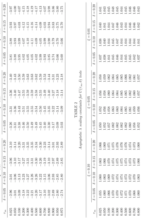
Asymptotic Size
We now consider the asymptotic sizes ofMDF( m; ) and U( m; ) under a local break in trend, for
the four window widths =f0:05;0:10;0:15;0:20g, and setting m= 0, so we assume the true break
fraction coincides with the mid-point of the window. In Figure 1 we show the sizes, as functions of the
local trend break magnitude =f0;0:2; :::;15g, for break fractions 0 =f0:3;0:5;0:7gat the nominal
0.05 level; for purposes of comparison, we also show the asymptotic sizes of DFGLS and the MDF1
procedure of HLT (i.e. MDF(0:5;0:7)).
The general pattern of results is as follows. Firstly, DFGLS displays the predictable feature of
its size rapidly decaying from 0:05 towards zero as increases, since a local trend break of growing
magnitude is being omitted from its underlying deterministic speci cation. TheMDF( m; ) statistics
have sizes which demonstrate quite di erent behaviour; their sizes increase from 0:05 as increases,
before levelling o then decreasing slightly. The maximum size is reached more rapidly in the
larger is ; but the maximum attained is higher the smaller is .5 The correspondingU( m; ) testing
strategies demonstrate sizes that are fairly close to 0:05 across all - they are all slightly undersized for > 0, though with less undersizing the smaller is . What is happening here is that, as is increasing, any over-sizing inherent in MDF( m; ) is being counteracted by the diminishing size of
DFGLS.6 The sizes of the U( m; ) strategies are pretty much in line with those of the HLT test MDF1 when 0 = 0:3 and 0 = 0:5, but are less undersized when 0 = 0:7.
By way of a more comprehensive check on the asymptotic size properties of theU( m; ) strategies,
we simulated the limit distribution of DFGLSU in (6) using the values of Table 2, that, is those
calculated for = 0, across a grid of values =f0;1;2; :::;15g and 0 = f0:025;0:050; :::;0:975g for
every case considered in Table 2 (i.e. each m, and signi cance level combination). This allows us to
examine size in cases where (i) m= 0, (ii) 0 2 ( m; ), m 6= 0 such that the partial information
on break location remains true but the break no longer occurs at the mid-point of the window, and
(iii) 0 2= ( m; ) so that the partial information is entirely wrong. The pertinent nding of this
analysis is that, for any given signi cance level, the maximum asymptotic size obtained across all
5For = 0:05, the maximum size is not obtained until = 30 at which point the size is 0:086.
6Note that although the size ofU for = 0:05 is still rising slightly when = 15, its size reaches a ceiling of 0:049
m, combinations considered was always within 0:0009 of the nominal level, thereby con rming the
suitability of the values of Table 2 to deliver what is, to all intents and purposes, a size-controlled
procedure.7
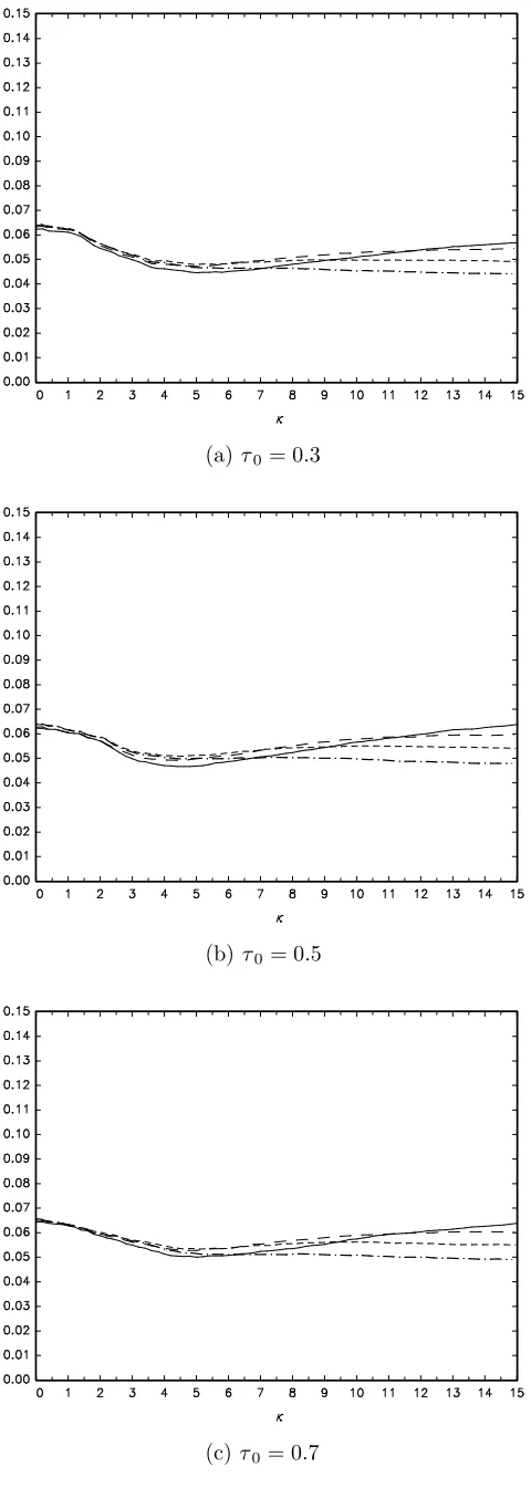
Asymptotic Power
Figure 2 plots the asymptotic local power functions of nominal 0.05 level tests across =f0;0:2; :::;15g, with m = 0 = f0:3;0:5;0:7g, for the two alternatives c = 20 and c = 25. We do not report plots
for the MDF( m; ) statistics alone (other than MDF1), since these are oversized. The results may
be summarized as follows. The power of DFGLS starts at a high level, but then decays towards zero
as increases, due to the increasing magnitude of the unattended break. As regards the U( m; )
testing strategies, for all four settings considered we observe that they are all able to harness most
of the high power available from DFGLS for zero or small values of , as well as power arising from
MDF( m; ). Then, as further increases, their power drops down to a lower level since the power
contribution ofDFGLS is declining towards zero and all their power is obtained from theMDF( m; )
statistics alone. Outside of small values of , that is, in the region whereMDF( m; ) and notDFGLS
dominates the power pro le, it becomes quite clear that the smaller is , the higher is the power which
is achieved.
The non-union test MDF1 cannot access any of the high power associated withDFGLS for zero or
very small values of . For the larger values of , when 0= 0:3 and 0 = 0:5, theU( m; ) strategies
are more powerful thanMDF1 apart from when = 0:20, where the power is marginally lower. When
0 = 0:7, all theU( m; ) strategies have substantially higher power thanMDF1, for large (as well as
small) .
We therefore see that the more accurate the true partial information available regarding the location
of the trend break (i.e. the smaller is ), the higher the power that can be achieved with U( m; ).
As we might expect, the level of information accuracy has little e ect on power when the local break
does not occur, or is small, but allows for very decent power gains otherwise.
Asymptotic Behaviour when m 6= 0
Finally, we jointly investigate the size and power properties of U( m; ) when m 6= 0. Here we set
0 = 0:57 and m = 0:50 such that = 0:15 and = 0:20 correspond to case (ii) discussed in the
rst sub-section above, with the break being "least central" for = 0:15; and such that = 0:05 and
= 0:10 correspond to case (iii), with the partial information being "most in error" for = 0:05. Asymptotic sizes forU( m; ) are given in Figure 3(a). The sizes forU( m; ) with =f0:15;0:20g
across are always very close to their counterparts for m = 0 = 0:5 in Figure 1, indicating that the
issue of whether or not the break occurs towards the window midpoint has little e ect on size. For
=f0:05;0:10g, the sizes approach zero in , and this occurs particularly quickly for = 0:05, where
the partial information is the more incorrect. In Figure 3(b) we present the corresponding powers for
c= 20. Once more we see that the power pro les forU( m; ) with =f0:15;0:20g lie very close to
their counterparts for m = 0 = 0:5 in Figure 2, while the powers for =f0:05;0:10g are decreasing
in , reaching zero for = 0:05.
From this analysis we make two observations. First, that the asymptotic size and power are little
a ected by the placement of a break within a given window, which endows theU( m; ) strategy with
a degree of robustness. Secondly, and not surprisingly, that size and power are both driven towards
zero by false partial information (more quickly when the more in error is that information). While
this may be considered a negative, we can at least rest assured that our strategy is very unlikely to
yield spurious rejections of the unit root null when one is present but the trend break exists outside
of the chosen window.
4
Finite Sample Results
In this section we present nite sample simulation results for the empirical size and power of the
U( m; ) tests. We setT = 200 and simulate the DGP given by (1) and (2) with = = 0 (without
loss of generality), "t IIDN(0;1) and u1 = "1. We use the same local trend break magnitudes
as in the previous section, and the same choices for 0. As in the rst two sub-sections of section 3
we set m = 0 and consider the four window widths =f0:05;0:10;0:15;0:20g. The Dickey-Fuller
regressions are implemented withk set to zero in (3), thereby abstracting from issues of lag selection.
Figures 4 and 5 report, respectively, the size (c = 0) and local power (c = 20;25) of the U( m; )
testing strategies, with the tests conducted using nominal 0.05 level asymptotic critical values and the
corresponding union of rejections scaling constants.
We nd that the reliable asymptotic size performance of theU( m; ) strategies is largely replicated
in the nite sample situation. The relative size pro les across for the four settings of follow the
same pattern as was observed for the limit case in Figure 1. The sizes forT = 200 are a little above the nominal level for some values of , but such oversizing is very moderate, never being in excess of
0:066.
Turning now to the nite sample power results of Figure 5, we again observe the same relative
power rankings among the four union of rejections strategies as in the limit, i.e. very similar power
for all values of when the local break magnitude is zero or very small, but then for larger , power
increases as the window width narrows. The level of nite sample power for each strategy is a little
higher than the corresponding local asymptotic power level, as expected given the moderate degree
of nite sample oversize observed in Figure 4. Overall then we nd that the attractive asymptotic
properties of the U( m; ) testing strategies carry over to the nite sample context, reinforcing the
5
An Empirical Illustration
By way of an illustration of the how theU( m; ) strategies might work in practice, we applied them to
UK interest rate data. The interest rate series we consider is the natural log of the monthly gross at
yield on UK government 2.5% Consols for the period January 1954 to November 1994.8 The series, comprising 491 observations, is shown in Figure 6. Observation 238, located near the middle of the
series (and also indicated in Figure 6), represents October 1973, the month in which the Middle East
Oil Crisis began. Few would argue that the period around the Oil Crisis should not be considered a
serious candidate for the location of a potential trend break in the long-term behaviour of economic
and nancial markets. Arguably, it was the most seismic economic event of the twentieth century,
aside from the Great Depression.
In what follows all ADF statistics are implemented with the MAIC lag selection procedure of Ng
and Perron (2001) and Perron and Qu (2007), usingkmax=b12(T =100)1=4c = 17. All test procedures
are carried out at the nominal 0.05 level, using asymptotic critical values and scaling constants.
As a benchmark, we took the view that a trend break did occur in October 1973. That is,
we assumed complete knowledge of the break location. The appropriate unit root statistic is then
DFGLS( ) with = 238=491 = 0:485. We found that this statistic does not yield a rejection of the unit root null. Moving to the other extreme, we eschewed all relevant information on break location
around the occurrence of the Oil Crisis and calculated the MDF1 test of HLT, i.e. MDF(0:5;0:7).
This test did not reject the unit root null either.9
To examine whether taking a partial information position might uncover evidence of stationarity
around a broken trend, we then calculatedU( m; ) for =f0:05;0:10;0:15;0:20g. Intuition led us to
set m= 0:485 such that each break window midpoint is xed at October 1973, thereby incorporating
the e ects of uncertainty caused by both anticipation (before) and delayed reactions (after) this date.
However, we also calculated U( m; ) setting m =2 = 0:485, so that October 1973 is now always
the earliest date in the window (the midpoint now varies) to allow for e ects of delayed reactions alone
(in keeping with the the Oil Crisis being termed a \shock" in the vernacular).
The results are shown in Table 3, whereNRandRdenote non-rejection and rejection, respectively,
of the unit root null at the 0.05 level. In analyzing these results, it should be borne in mind that the
DFGLS component of each U( m; ), i.e. the without break unit root test, is never responsible for
triggering a rejection; its value is 0.90, compared with a critical value of 2.85, even before any
scaling is applied. Therefore, the pattern of rejections in Table 3 is solely within the purview of the
corresponding with-break MDF( m; ) component ofU( m; ).
If we set m = 0:485 then only the = 0:15 window yields a rejection. It seems reasonable to
argue, informally at least, that this arises because the =f0:05;0:10g windows are excluding a true
break point which is contained in the = 0:15 window. Of course, this break point is also included
8This same data set was examined by Leybourneet al. (1998) in the context of unit root tests allowing for smooth transition trend deterministics.
9
in the = 0:20 window, but the price here is a more left-shifted critical value, which overturns the rejection. Once we set m =2 = 0:485 we no longer consider pre-October 1973 dates as candidate
break points for any window. The = 0:15 window still produces a rejection but is now joined by rejections for the =f0:05;0:10gwindows, which leads us to presume that both of these now include
the trend break point. Interestingly, the = 0:20 window also now yields a rejection. Essentially, this is because the rightward shift of the window midpoint (relative to m= 0:485) means the critical
value is less left-shifted.10
Our ndings lead us to conclude that this interest rate series is stationary, around a trend break,
though it would seem that the break point appears much less likely to have occurred before the onset
of the Oil Crisis than at some stage shortly thereafter. It therefore seems doubtful that the Oil Crisis
was anticipated by the bond market to any appreciable extent. In fact, our results with window width
= 0:05 suggest that the trend break occurred between observations 251 and 262; that is, between November 1974 and October 1975.11 Visual inspection of Figure 6 would not appear to contradict this suggestion.
6
Conclusions
In this paper we have proposed a union of rejections-based approach to testing for a unit root when
partial information is available regarding the location, but not necessarily the presence, of a break in
linear trend. The union of rejections approach, comprised as it is of both a with-break and
without-break unit root test, allows the capture of most of the high power available when no without-break is actually
present, while also ensuring a reliable level of power should a break occur. Our recommended approach
relies on the user specifying a window within which the putative trend break must lie, and the narrower
this window width is, the greater is the level of power achievable for non-zero break magnitudes. Our
results demonstrate that this new approach can outperform existing approaches and delivers a reliable
procedure for testing for a unit root when such partial information is available. Of course, the decision
regarding the window width and location lies with the practitioner, and should re ect their degree of
belief regarding the approximate date of any trend break that might occur. While the obvious caveat
exists that a mis-speci ed window choice could result in low power, we think that this new procedure
has attractive properties, and should prove desirable to users. Our procedure can be seen as bridging
the gap between an often unrealistic assumption that the putative trend break date is known with
complete certainty, and the highly conservative assumption of no knowledge whatsoever regarding
the break location; both extremes being rather unappealing for many events likely to generate trend
breaks in economic or nancial data.
10
This window midpoint is actually now m = 0:585 instead of 0:485. Table 1 shows that the critical value of MDF( m; ) changes to 3:59 from 3:62. In addition, from Table 2, the scaling reduces to 1:062 from 1:066.
References
Andrews, D. W. K. (1993). `Tests for parameter instability and structural change with unknown
change point', Econometrica, Vol. 61, pp. 821{856.
Banerjee, A., Lumsdaine, R. and Stock, J. (1992). `Recursive and sequential tests of the unit root and
trend break hypotheses: theory and international evidence',Journal of Business and Economics
Statistics, Vol. 10, pp. 271{288.
Carrion-i-Silvestre, J. L., Kim, D. and Perron, P. (2009). `GLS-based unit root tests with multiple
structural breaks both under the null and the alternative hypotheses',Econometric Theory, Vol.
25, pp. 1754{1792.
Elliott, G., Rothenberg, T. J. and Stock, J. H. (1996). `E cient tests for an autoregressive unit root',
Econometrica, Vol. 64, pp. 813{836.
Hanck, C. H. (2012). `Multiple unit root tests under uncertainty over the initial condition: some
powerful modi cations',Statistical Papers, forthcoming.
Harris, D., Harvey, D. I., Leybourne, S. J. and Taylor, A. M. R. (2009). `Testing for a unit root in
the presence of a possible break in trend',Econometric Theory, Vol. 25, pp. 1545{1588.
Harvey, D. I. and Leybourne, S. J. (2012). `An in mum coe cient unit root test allowing for an
unknown break in trend', Economics Letters, Vol. 117, pp. 298{302.
Harvey, D. I., Leybourne, S. J. and Taylor, A. M. R. (2009). `Unit root testing in practice:
deal-ing with uncertainty over the trend and initial condition (with commentaries and rejoinder)',
Econometric Theory, Vol. 25, pp. 587{667.
Harvey, D. I., Leybourne, S. J. and Taylor, A. M. R. (2011). `Testing for unit roots in the possible
presence of multiple trend breaks using minimum Dickey-Fuller statistics', Manuscript, School
of Economics, University of Nottingham. Downloadable fromhttp://www.nottingham.ac.uk/
lezdih/papers.htm.
Harvey, D. I., Leybourne, S. J. and Taylor, A. M. R. (2012a). `Testing for unit roots in the presence
of uncertainty over both the trend and initial condition',Journal of Econometrics, Vol. 169, pp.
188{195.
Harvey, D. I., Leybourne, S. J. and Taylor, A. M. R. (2012b). `Unit root testing under a local break
in trend', Journal of Econometrics, Vol. 167, pp. 140{167.
Harvey, D. I., Leybourne, S. J. and Taylor, A. M. R. (2012c). `On in mum Dickey-Fuller unit root
tests allowing for a trend break under the null', Manuscript, School of Economics, University of
Kim, D. and Perron, P. (2009). `Unit root tests allowing for a break in the trend function at an
unknown time under both the null and alternative hypotheses', Journal of Econometrics, Vol.
148, pp. 1{13.
Leybourne, S. J., Newbold, P. and Vougas, D. (1998). `Unit roots and smooth transitions',Journal
of Time Series Analysis, Vol. 19, pp. 83{97.
Ng, S. and Perron, P. (2001). `Lag length selection and the construction of unit root tests with good
size and power', Econometrica, Vol. 69, pp. 1519{1554.
Perron, P. (1997). `Further evidence of breaking trend functions in macroeconomic variables',Journal
of Econometrics, Vol. 80, pp. 355{385.
Perron, P. and Qu, Z. (2007). `A simple modi cation to improve the nite sample properties of Ng
and Perron's unit root tests',Economics Letters, Vol. 94, pp. 12{19.
Perron, P. and Rodr guez, G. (2003). `GLS detrending, e cient unit root tests and structural change',
Journal of Econometrics, Vol. 115, pp. 1{27.
Perron, P. and Vogelsang, T. J. (1992). `Nonstationarity and level shifts with an application to
purchasing power parity',Journal of Business and Economic Statistics, Vol. 10, pp. 301{320.
Zivot, E. and Andrews, D. W. K. (1992). `Further evidence on the great crash, the oil-price shock, and
TABLE 3
Application of U(τm, δ) at the nominal 0.05-level to yield on UK 2.5% Consols
δ τm = 0.485 τm−δ/2 = 0.485
0.05 NR R
0.10 NR R
0.15 R R
(a)τ0= 0.3
(b)τ0= 0.5
[image:16.595.178.437.41.761.2](c)τ0= 0.7
Figure 1. Asymptotic size: DFGLS: · · ·H· · ·, MDF1: ;
U(τ0,0.05): ,U(τ0,0.10): – – , U(τ0,0.15): - - -, U(τ0,0.20): – · – ;
(a)c= 20,τ0= 0.3 (b)c= 25,τ0= 0.3
(c)c= 20,τ0= 0.5 (d)c= 25,τ0= 0.5
[image:17.595.49.547.41.750.2](e)c= 20,τ0= 0.7 (f)c= 25,τ0= 0.7
(a)c= 0 (b)c= 20
Figure 3. Asymptotic size and local power, τ0 = 0.57:
(a)τ0= 0.3
(b)τ0= 0.5
[image:19.595.178.418.48.725.2](c)τ0= 0.7
Figure 4. Finite sample size, T = 200, ρT = 1, γT =κT−1/2:
(a)c= 20,τ0= 0.3 (b)c= 25,τ0= 0.3
(c)c= 20,τ0= 0.5 (d)c= 25,τ0= 0.5
[image:20.595.52.543.61.724.2](e)c= 20,τ0= 0.7 (f)c= 25,τ0= 0.7
Figure 5. Finite sample power, T = 200,ρT = 1−c/T,γT =κT− 1/2