Reconstruction of Wireless UWB Pulses by Exponential Sampling Filter

doi:10.4236/wsn.2010.26057 Published Online June 2010 (http://www.SciRP.org/journal/wsn)

Reconstruction of Wireless UWB Pulses by Exponential

Sampling Filter

Juuso T. Olkkonen1_{, Hannu Olkkonen}2 1_{VTT Technical Research Centre of Finland, Espoo, Finland}

2_{Department of Physicsand Mathematics, University of Eastern Finland, Kuopio, Finland} E-mail: [email protected], [email protected]

Received November 16, 2009; revised December 25,2009; accepted January 20,2010

Abstract

Measurement and reconstruction of wireless pulses is an important scheme in wireless ultra wide band (UWB) technology. In contrary to the band-limited analog signals, which can be recovered from evenly spaced samples, the reconstruction of the UWB pulses is a more demanding task. In this work we describe an exponential sampling filter (ESF) for measurement and reconstruction of UWB pulses. The ESF is con-structed from parallel filters, which has exponentially descending impulse response. A pole cancellation filter was used to extract the amplitudes and time locations of the UWB pulses from sequentially measured sam-ples of the ESF output. We show that the amplitudes and time locations of p sequential UWB pulses can be recovered from the measurement of at least 2p samples from the ESF output. For perfect reconstruction the number of parallel filters in ESP should be 2p. We study the robustness of the method against noise and dis-cuss the applications of the method.

Keywords:Wireless Sensor Networks, UWB, Network Security, Finite Rate of Innovation

1. Introduction

The measurement and reconstruction of some classes of signals containing discontinuities such as impulses and edges is difficult [1,2]. Sampling methods are historically relied on Shannon’s theorem [3]. The perfect reconstruc-tion (PR) of the continuous signal from the sampled ver-sion requires that the signal is band limited, i.e., its fre-quency spectrum has a maximum frefre-quency f_M. The PR is possible only if the sampling frequency f_s2f_M . For example, signals in optical devices and radiation detec-tors are not band limited and classical sampling ap-proaches are not relevant for extracting the information.

Sampling scheme with finite rate of innovation (FRI) [4,5] has recently got vast interest in signal processing society, since the FRI methods are not restricted to the recovery of the band-limited signals. The key idea in FRI methods is that the signal (e.g.,the Dirac impulse stream) is measured with a sampling filter, which is constructed using analog circuits. The output of the sampling filter is measured and the original signal is reconstructed from the discrete samples. Excellent articles and reviews con- sider the FRI sampling and reconstruction techniques

[4-9] and many feasible applications have been published. However, the experimental work on the verification of the underlying theoretical considerations is lacking, espe-cially the effect of noise on the reconstruction accuracy.

The information in wireless ultra wideband (UWB) devices is usually carried out by monocycle Gaussian pulses. In year 2002 the FCC restricted the allowed fre-quency band between 3.1-10.6 GHz for unlicensed UWB transmission [10]. The monocycle Gaussian pulse stream does not strictly meet this constraint and other pulse shapes have been introduced, e.g., the family of the or-thogonal UWB pulse waveforms [11]. In low-range wireless UWB communication devices, which transmit sequential pulses, the information is coded to the time locations of the pulses. The UWB pulse generators are relatively easy to implement in VLSI [12]. The pulse stream is designed so that its power spectral density co-incides with the FCC criteria.

2. Theoretical Considerations

2.1. Sampling of the UWB Pulse Train

We consider the UWB pulse train, which is approximated by

1

( ) ( )







p _i  _i i

I t A t t (1)

where the Dirac distribution ( ) 1 for x  x0 and

( ) 0 for x x 0

   . denotes the amplitude and time location. The pulse train is fed to the exponential sampling filter (ESF) consisting of N parallel RC-filters (Figure 1). The ESF has the causal impulse response

i

A

t

_i

1

( ) exp[ ] 0







N _k  k

h t B kt t (2)

The output signal of the ESF is

1 1

( ) ( ) ( ) ( ) ( )

exp[ ( )] 0

p N

i k i

i k

x t I t h t I h t d

A B k t t t

              



 

  (3)

The key idea is to start the measurement of the ESF output at time , simultaneously clos-ing the input of the ESF (Figure 1). We define the dis-crete time variable n as

0 i( 1, 2,..., )

t t i p

0 ( 0,1, 2,...

  

t t nT n ) nT t t0

where T is a sampling period. For the samples of the ESF output x_nx nT n[ ], 0,1, 2,... the following is valid

0

1 1

exp[ ( )]

 



 

p N  

n i k i

i k

x A B k t nT t (4)

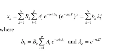
[image:2.595.309.515.65.153.2]

By rearranging and denoting   _i t_o t_i

Figure 1. The construction of the ESF from the parallel exponential filters (EF), which are built using RC-circuits. The ESF parameter is related as , where and are the component values.

 αkT1 / (R C )k k k

R Ck

1 1 1

( )

  

  



 

i 



p

N N

k k T n n

n k i k

k i k

x B A e e bk (5)

where

1

and

  







i 

p

k kT

k k i k

i

b B A e _ e  ₍₆₎

2.2. Reconstruction of the Pulse Train

Our task is to recover the amplitudes and time loca-tions of the pulses from the measured output samples

[ ], 0, 1, 2,...

 

n

x x nT n We may write (5) in the form

of matrix/vector equation

0 1

2 1 2

1 1 1

1 1 2

1 1 1

N

N N N

N N 2 N x b x b x b                         _                     

 _{x λb} _{b λ}-1_x  

    



 (7)

The Vandermonde matrix structure in (7) is non-singular having rank N and the solution of the vector requires knowledge of the N measurement values. From (6) we obtain

λ

b

1 1

/   =

 

 



i



p p

k k

k k k i i i

i i

c b B A e A r (8)

where

 

 i i

r e (9) The z transform of the

c

_k sequence gives

 

1

1 1

1 1 1 0

1 1 1 = ( ) (1 ) 1 p p N N

k k k

k i i i i

k i i k

N N p

i i i

i i

Z c A r z A r z

A r z r z r z                   



  (10)

We define the pole cancellation filter (PCF) as

1

1 1

( ) 1  (1 )

 

 



p n 



p 

pc n j

n j

H z h z r z (11)

where rj is defined by (9). Next we consider the prod-uct filter P z( )

 

1 1

1 1

( ) ( )

(1 ) (1 )

k pc p p

N N

i i i j

i j

j i P z Z c H z

A r z r z r z

    







  k h (12)

We may note that the roots of the equal the roots of the PCF. The impulse response of the is

( ) P z ( ) P z 0   



p

n n k

k

p c (13)

For solution of the roots of the P z( ) we setp_n0 for . This yields the matrix/vector equation

0





2 2 1 2 2 1

2 1 2 2 2 3 1 2

1 1 1

0

p p p p

p p p p

p p p p

c c c c h

c c c c h

c c c c h

                      _                           

  _{c Ch} _{h C c}-1

         － (14)

We may note that the solution of the p coefficients of the PCF requires the knowledge of the 2p values of the

sequence. The polynomial

k

c

[1h h1 2hp]

p

has the roots   i , which give

i

r e (i1, 2,..., )   _i log ( )r_i / and the time locations as t_i t₀ log( ) /r_i  . For solution of the amplitudes we may write (8) in ma-trix/vector form

1 1 2 1

2 2 2

1 1 2 2

1 2

p

p

p p p

p p

c r r r A

c r r r A

c r r r A

              _                           

 _{c R a} _{a R c}-1

         _p p ] (15)

To summarize, the reconstruction of p sequential pulses needs the measurement of at least 2p samples from the ESF output. The impulse response of the ESF must obey (2), where . It should be pointed out that the solution of the matrix Equations (7) and (15) require the inversion of the Vandermonde matrix, which can be ob-tained by an analytical formula [13]. The inversion method yields more stable results compared with the general matrix inversion.

2



N

2.3. Reduction of Noise

In practical measurements noise arising in electronic circuits interferes the results. We apply the SVD based subspace method for reducing the noise in measurement signal. Let us construct the Hankel matrix containing the measurement values x_nx nT[ , (n0,...,M 2 )p

1       n

0 1 / 2

1 2 / 2

/ 2 / 2 1

                M M

M M M

x x x

x x x

x x x

H (16)

where the antidiagonal elements are identical. The sin- gular value decomposition (SVD) of the matrix H is

T

H = UΣV (17) where and are unitary matrices. is a diago- nal matrix consisting of the singular values in descending order. The decomposition (17) can be separated as

U V Σ





 





    T s s n s n n T T

s n s

s s n n

0 Σ

H = U U ₀ V V Σ

= U Σ V U Σ V = H H

(18)

where contains the smallest singular values. matrix belongs to noise subspace. The matrix is then related to the noise free signal subspace [14]. The signal matrix is not precisely Hankel matrix, but some variation occurs in the antidiagonal elements. We re-constructed the noise free Hankel matrix by replacing the antidiagonal elements by their mean values. This enables the computation of the noise cancelled xn

n Σ s H 1,..., n H s H

(n0, M) sequence. The dimension of the signal subspace is N, i.e., the number of parallel RC-circuits in ESF. It should be pointed out that the Hankel matrix (16) must be a full matrix. Therefore M should be even.

3. Experimental

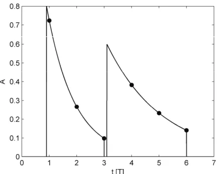
Extensive simulations were performed to validate the theoretical results. The T parameter in (5) varied between 0.1-0.3. The number of the impulses in one burst varied between 3-7 and the number N in ESF (2) in the range 3-15. The amplitudes of the pulses were randomly distributed between the limits 0.1-0.9. The simulations warranted the condition that for the recovery of p pulses at least 2p samples are needed in the de- scending part of the ESF output. A typical simulation study is illustrated in Figure 2. In every case the ESF method recovered the amplitudes and the time locations of the pulses with a machine precision.

A prototype ESF was constructed with the aid of six parallel RC-circuits (Figure 1). The output was measured by a 16 bit analog-to-digital converter (ADC), which was equipped with a sample and hold amplifier (S/H). The input of the ESF was closed using the analog CMOS switch. The ESF was reset by grounding the output by an analog CMOS switch. Using a commercial UWB pulse generator two sequential pulses were fed to the input of the ESF and the descending part was meas-ured with a 40 MHz sampling frequency. Due to the noise interference in practical measurements the use of the SVD based noise suppression method was essential. The prototype ESF recovered the amplitudes and the appearance times with a good accuracy. The mean error (standard deviation divided by the mean value) in ampli-tudes was 2.7% and in time locations 0.2%.

4. Discussion

[image:4.595.64.282.77.251.2]

Figure 2. The minimum time interval i i i1 must be for perfect reconstruction using ESF with two parallel RC circuits and three sequential samples per im-pulse. The dashed circles denote the measurement values and the solid line reconstructed ESF output via Equation (3).

dt  t t

2 i

dt  T

of the samples was proved to be at least 2p. The simu- lations using noise free signal indicated an accurate and precise reconstruction property, in practice the ESF me- thod showed a high sensitivity to the noise. To obtain a tolerable reconstruction error, the ESF circuit requires Faraday gage-type shielding and careful consideration of grounding and signal cables. The experimental verifica-tion of the effect of different types of noise sources (50 Hz + harmonics pick-up, 1/f-noise and random noise) needs further study.

In this work the noise was cancelled using the SVD based subspace method (16-18), which eliminates the noise interference if the number of samples exceeds 2p. The key idea is to compute the noise free signal as a mean of the antidiagonal elements in the signal subspace matrix H_s. The error in the noise cancelled sequence

0, 1, (  ..., )

n

x n M attains a minimum in the middle of the sequence, where M data points are used for computa-tion of the mean value. Evidently the higher error in both ends of the sequence is due to the lower number of points.

The ESF method has a close relationship with the FRI methods, which are based on the sequential measurement of the output of the analog circuit network [5]. The re-construction properties of the Gaussian, sinc-type and triangle-wave sampling filters have been described [4-6, 8], but to the best of the authors knowledge, ESF-type circuits have not been previously used for the sampling and recovery of the UWB pulse sequences. A clear dif-ference between the FRI sampling filters and the ESF comes from causality. An exponential impulse response

exp[k t t(  _i)] is causal and can be separated in (5)

only if . On the contrary, FRI sampling filters are not causal and this restriction is not needed in the deduction of the reconstruction algorithms. The FRI reconstruction algorithms usually require the solution of two matrix/vector equations, which are Yale-Walker and Vandermonde structures. In our approach three matrix/ vector solutions (7, 14, 15) are required.

 _i

t t

The present ESF measurement scheme can be consid-ered as a general framework for measurement of the UWB pulse amplitudes and time locations. The experi-ments showed that the reconstruction error is mainly due to the additive random noise affecting on the amplitudes of the pulses. Hence, as an example of the practical con-struction of the wireless sensor network the ratio of the two sequential UWB pulse amplitudes can be related to the device address. The ratio of the UWB pulse ampli-tudes is not affected by the attenuation and distance variations. The time difference between the UWB pulses is reconstructed more accurately and it can be used to code the transmitted information.

The ESF method can be applied in many areas of wireless sensor technology and instrumentation. For example, in optical instruments the time difference be-tween laser pulses can be used in testing light transmis-sion in optical fibres. Many other sensors have pulse- type outputs.

5. Acknowledgements

This work was supported by the National Technology Agency of Finland (TEKES).

6. References

[1] J. Haupt and R. Nowak, “Signal Reconstruction from Noisy Random Projections,” IEEE Transactions Information The-ory, Vol. 52, No. 9, 2006, pp. 4036-4048.

[2] Y. C. Eldar and M. Unser, “Nonideal Sampling and In-terpolation from Noisy Observations in Shift-Invariant Spaces,” IEEE Transactions Signal Processing, Vol. 54, No. 7, 2006, pp. 2636-2651.

[3] M. Unser, “Sampling-50 Years after Shannon,” Procee- dings of IEEE, Vol. 88, No. 4, 2000, pp. 569-587. [4] P. Marziliano, “Sampling Innovations,” Ph.D. Dissertation,

Communications laboratory, Lausanne, Switzerland, 2001. [5] M. Vetterli, P. Marziliano and T. Blu, “Sampling Signals

with Finite Rate of Innovation,” IEEE Transactions Sig-nal Processing, Vol. 50, No. 6, 2002, pp. 1417-1428. [6] I. Maravic and M. Vetterli, “Sampling and Reconstruc-

tion of Signals with Finite Rate of Innovation in the Presence of Noise,” IEEE Transactions Signal Process- ing, Vol. 53, No. 8, 2005, pp. 2788-2805.

Shot Noise,” IEEE Transactions Information Theory, Vol. 52, No. 5, 2006, pp. 2230-2233.

[8] P. L. Dragotti, M. Vetterli and T. Blu, “Sampling Mo-ments and Reconstructing Signals of Finite Rate of Inno-vation: Shannon Meets Strang-Fix,” IEEE Transactions Signal Processing, Vol. 55, No. 5, 2007, pp. 1741-1757. [9] I. Jovanovic and B. Beferull-Lozano, “Oversampled A/D

Conversion and Error-Rate Dependence of Nonband Li- mited Signals with Finite Rate of Innovation,” IEEE Transactions Signal Processing, Vol. 54, No. 6, 2006, pp. 2140-2154.

[10] Y. P. Nakache and A. F. Molisch, “Spectral Shaping of UWB Signals for Time-Hopping Impulse Radio,” IEEE Journal of Selected Areas of Communications, Vol. 24, No. 4, 2006, pp. 738-744.

[11] B. Parr, B. Cho, K. Wallace and Z. Ding, “A Novel Ul-tra-Wideband Pulse Design Algorithm,” IEEE Commu- nications Letters, Vol. 7, No. 5, 2003, pp. 219-221. [12] M. Miao and C. Nguyen, “On the Development of an

Integrated CMOS-Based UWB Tunable-Pulse Transmit Module,” IEEE Transactions Microwave Theory and Techniques, Vol. 54, No. 10, 2006, pp. 3681-3687. [13] V. E. Neagoe, “Inversion of the Van Der Monde Matrix,”

IEEE Signal Processing Letters, Vol. 3, No. 4, 1996, pp. 119-120.