A consistent determination of the temperature of the intergalactic
medium at redshift
z
=
2
.
4
James S. Bolton,
1‹George D. Becker,
2Martin G. Haehnelt
2and Matteo Viel
3,4 1School of Physics and Astronomy, University of Nottingham, University Park, Nottingham NG7 2RD, UK2Kavli Institute for Cosmology and Institute of Astronomy, Madingley Road, Cambridge CB3 0HA, UK 3INAF - Osservatorio Astronomico di Trieste, Via G.B. Tiepolo 11, I-34131 Trieste, Italy
4INFN/National Institute for Nuclear Physics, Via Valerio 2, I-34127 Trieste, Italy
Accepted 2013 December 5. Received 2013 October 22; in original form 2013 August 14
A B S T R A C T
We present new measurements of the thermal state of the intergalactic medium (IGM) atz∼2.4 derived from absorption line profiles in the Lyαforest. We use a large set of high-resolution hydrodynamical simulations to calibrate the relationship between the temperature–density (T–) relation in the IGM and the distribution of HIcolumn densities,NHI, and velocity widths,
bHI, of discrete Lyαforest absorbers. This calibration is then applied to the measurement of the
lower cut-off of thebHI–NHIdistribution recently presented by Rudie et al. We infer a
power-lawT–relation,T=T0γ−1, with a temperature at mean density,T0=[1.00+−00..3221]×104K
and slope (γ −1) =0.54±0.11. The slope is fully consistent with that advocated by the analysis of Rudie et al.; however, the temperature at mean density is lower by almost a factor of 2, primarily due to an adjustment in the relationship between column density and physical density assumed by these authors. These new results are in excellent agreement with the recent temperature measurements of Becker et al., based on the curvature of the transmitted flux in the Lyαforest. This suggests that the thermal state of the IGM at this redshift is reasonably well characterized over the range of densities probed by these methods.
Key words: intergalactic medium – quasars: absorption lines.
1 I N T R O D U C T I O N
The temperature of the intergalactic medium (IGM) represents a fundamental quantity describing the physical state of the majority of baryons in the Universe. In the standard paradigm, the thermal state of the low-density IGM, which gives rise to the Lyαforest in quasar spectra, is set primarily by the balance between photo-ionization heating and adiabatic cooling. At redshifts well after reionization completes, this should result in a well-defined power-law relationship between temperature and density,T=T0γ−1,
for overdensities=ρ/ρ ≤10 (Hui & Gnedin1997). During and immediately following hydrogen or helium reionization, in con-trast, the temperature–density relation will become multi-valued and spatially dependent (Bolton, Meiksin & White2004; McQuinn et al.2009; Meiksin & Tittley 2012; Compostella, Cantalupo & Porciani2013). It has been suggested that additional heating pro-cesses, such as volumetric heating by TeV emission from blazars, may modify this picture (Puchwein et al.2012, but see Miniati & Elyiv2013). Regardless of the precise heating mechanism, how-ever, the long adiabatic cooling time-scale at these low densities,
tad∝H(z)−1, means that the IGM retains a long thermal memory.
E-mail:[email protected]
The temperature–density (T–) relation can therefore serve as a powerful diagnostic of the reionization epoch and the properties of ionizing sources in the early Universe (e.g. Miralda-Escud´e & Rees 1994; Theuns et al.2002a; Hui & Haiman2003; Cen et al.2009; Furlanetto & Oh2009; Raskutti et al.2012).
Over the last decade there have been many attempts to measure the thermal state of the low-density IGM using the Lyα forest. These measurements may be broadly classed into two approaches: statistical techniques which treat the Lyα forest transmission as a continuous field quantity (Zaldarriaga, Hui & Tegmark 2001; Theuns et al.2002b; Bolton et al.2008; Viel, Bolton & Haehnelt 2009; Lidz et al.2010; Becker et al.2011; Garzilli et al.2012) and those that instead decompose the Lyα forest absorption into dis-crete line profiles (Haehnelt & Steinmetz1998; Schaye et al.2000; Ricotti, Gnedin & Shull2000; Bryan & Machacek2000; McDonald et al.2001; Bolton et al.2010,2012; Rudie, Steidel & Pettini2012a, hereafterRSP12). These studies have produced a variety of results, not all of which are in good agreement. The tension between the measurements has historically remained relatively weak, however, as the statistical and/or systematic uncertainties have often been large.
Recently, however, two studies based on large data sets have claimed to measure temperatures in the IGM atz=2.4 to high (<10 per cent) precision, but with apparently discrepant results.
2014 The Authors
at University of Nottingham on July 4, 2016
http://mnras.oxfordjournals.org/
The first was by Becker et al. (2011), who analysed the cur-vature of the transmitted flux in the Lyα forest over 2 < z < 5. This study measured the temperature at a characteristic over-density, T( ¯), where ¯evolved with redshift. At z= 2.4, they foundT( ¯)=[2.54±0.13]×104K (2σerror) at ¯=4.4. More
recently, RSP12 reported a measurement of theT– relation at
z = 2.37 using Lyα line profiles in a large set of high reso-lution, high signal-to-noise spectra obtained as part of the Keck Baryonic Structure Survey (KBSS, Rudie et al.2012b). They mea-sured a temperature at mean density,T0=[1.87±0.08]×104K,
and a power-law slope, (γ − 1)= 0.47± 0.10 (1σ errors), for their ‘default’ outlier rejection scheme. TheRSP12results imply a temperature at the density probed by Becker et al. (2011) of
T( ¯)=[3.75±0.58]×104K (1σ, including the errors in bothT 0
andγ−1), which is discrepant with the Becker et al. (2011) value at over the 2σlevel. Stated differently, for the Becker et al. (2011) value ofT( ¯) to be consistent with theRSP12value ofT0would
require (γ −1)=0.21±0.03, which is at odds with theRSP12 result for the slope of theT–relation.
Obtaining consistent measurements of the IGMT–relation at
z=2.4 would be a considerable step towards establishing the full thermal history of the high-redshift IGM, which is intimately related to hydrogen and helium reionization and to the characteristics of ionizing sources. For example, the value for the slope of the T–
relation advocated byRSP12 is in good agreement with that expected for an optically thin, post-reionization IGM, where the temperature is set by the balance between adiabatic cooling and photo-heating only. This implies there may be no need for the additional heating processes which have been invoked to explain the observed probability distribution function (PDF) of the Lyα forest transmission at 2< z < 3 (Bolton et al.2008; Viel et al. 2009).
One possible avenue towards reconciling the Becker et al. (2011) andRSP12results is to re-examine the calibrations underlying their temperature results. Becker et al. (2011) employed a suite of hydro-dynamical simulations to convert their curvature measurements to temperatures at a specific overdensity.RSP12obtained their mea-surement of theT–relation using the velocity width–column den-sity (bHI–NHI) cut-off technique developed by Schaye et al. (1999)
(hereafterS99). This latter approach is based on the premise that the lower envelope of thebHI−NHI plane arises from gas which follows theT–relation of the IGM.S99used hydrodynamical simulations to establish and calibrate the relationship between the
bHI–NHI cut-off and theT–relation. In contrast to the original S99analysis, however,RSP12obtained their measurements using an analytical expression for the relationship between andNHI and the assumption that Lyαabsorption lines at thebHI–NHIcut-off are thermally broadened.
In this work we revisit the calibration of the bHI–NHI cut-off technique used byRSP12. Specifically, we use a large set of high-resolution hydrodynamical simulations of the IGM to test the ro-bustness of the values of T0 and (γ − 1) advocated by RSP12
based on their measurement of the lower cut-off in thebHI–NHI distribution. Our goals are two-fold. First, we wish to confront the analytical approach adopted byRSP12with detailed simulations of the IGM. Secondly, using these simulations, we may assess whether theRSP12measurement is consistent with other recent results, or whether there is genuine tension between measurements of the IGM thermal state at 2< z <3 obtained using Lyαtransmission statistics and line decomposition techniques.
We note that this redshift range represents an excellent starting point for establishing a consensus picture of the thermal state of
the high-redshift IGM, for multiple reasons. First, it is after the end of helium reionization (e.g. Shull et al.2010; Syphers et al.2011; Worseck et al.2011), when theT–relation at low densities can reasonably be expected to follow a power law. Secondly, excellent high-resolution spectra covering the Lyαforest can be obtained from bright quasars. Critically, the Lyαforest is also relatively sparse at these redshifts, enabling a largely straightforward decomposition of the forest into individual absorption lines and thus an analysis of the temperature as a function of density using thebHI–NHIcut-off technique.
We begin by providing a brief overview of the numerical simu-lations and methodology in Section 2. Our results are presented in Section 3 and a discussion follows in Section 4. A numerical con-vergence test of thebHI–NHIcut-off measured in the simulations is presented in an Appendix.
2 M E T H O D O L O G Y
2.1 Hydrodynamical simulations and Lyαforest spectra
In order to calibrate the relationship between the observedbHI–
NHI cut-off and the IGMT–relation, we utilize cosmological hydrodynamical simulations performed usingGADGET-3 (Springel
2005). The bulk of the simulations used in this study are described by Becker et al. (2011) (see their table 2). In this work we supplement these models with four additional runs which explore a finer grid of (γ −1) values. This gives a total of 18 simulations for use in our analysis, all of which have a box size of 10h−1comoving Mpc, a
gas particle mass of 9.2×10⁴h−1M
and follow a wide range of IGM thermal histories characterized by differentT–relations. The cosmological parameters adopted in the simulations arem=0.26,
=0.74,bh2=0.023,h=0.72,σ8=0.80,ns=0.96, with
a helium mass fraction ofY=0.24. We shall demonstrate later our results remain insensitive to this choice by instead using the recent Planck results [Ade et al. (Planck Collaboration XVI)2013].
Mock Lyαforest spectra are extracted from the simulations from outputs atz=2.355 and are processed to match theRSP12 observa-tional data (e.g. Theuns et al.1998). The mean transmitted flux,F, of the spectra is matched to the recent measurements presented by Becker et al. (2013). The simulated data are then convolved with a Gaussian instrument profile with FWHM=7 km s−1and rebinned
on to pixels of width∼3 km s−1to match the Keck/HIRES
spec-trum characteristics ofRSP12. Finally, Gaussian distributed noise is added with a total signal-to-noise ratio (S/N) of 89, matching the mean S/N of theRSP12data.
2.2 FrombHI–NHIcut-off toT–relation
The procedure used for measuring thebHI–NHIcut-off in the sim-ulations follows the method described inS99andRSP12. We use
VPFIT1to fit Voigt profiles to our mock Lyαforest spectra. We then select a sub-sample of the lines using the ‘default’RSP12 selec-tion criteria: only absorbers with 8≤bHI/[km s−1]≤100, 1012.5≤
NHI/[cm−
2]≤1014.5and relative errors of less than 50 per cent are
included. We furthermore ignore all lines within 100 km s−1 of
the edges of our mock spectra to avoid possible line duplications arising from the periodic nature of the simulation boundaries. We note, however, that we opted not to use the additionalσ-rejection
1Version 10.0 by R.F. Carswell and J.K. Webb, http://www.ast.
cam.ac.uk/∼rfc/vpfit.html
at University of Nottingham on July 4, 2016
http://mnras.oxfordjournals.org/
scheme introduced by RSP12. We found this procedure did not work effectively when applied to models withbHI–NHI distribu-tions which differed significantly from theRSP12data. We therefore always compare to theRSP12‘default’ measurements throughout this work.
The power-law cut-off at the lower envelope of thebHI–NHIplane,
bHI=bHI,0(NHI/NHI,0)−1, is then measured in each of our
simu-lations by applying the iterative fitting procedure described byS99 to 4000 Lyαabsorption lines selected following the above criteria (the fullRSP12sample contains 5758 HIabsorbers). Uncertainties
onb0and (−1) are estimated by bootstrap sampling the lines
with replacement 4000 times.
Once thebHI–NHIcut-off has been measured in the simulations, theT–relation may then be inferred by utilizing the ansatz tested byS99– namely that power-law relationships hold between–NHI andT–bHIfor absorption lines near the cut-off, such that
log=ζ1+ξ1log(NHI/NHI,0), (1)
logT =ζ2+ξ2logbHI. (2)
Substituting these expressions into theT–relation and comparing coefficients with the power-law cut-off,bHI=bHI,0(NHI/NHI,0)−1,
we identify,
γ−1= ξ2
ξ1
(−1), (3)
logT0=ξ2logbHI,0+ζ2−ζ1(γ−1), (4)
whereζ1=0 whenNHI,0is the column density corresponding to
gas at mean density. A measurement ofT0and (γ −1) therefore
relies on correctly identifying the remaining three coefficients in equations (1) and (2), andadditionally,NHI,0. Selecting a value of
NHI,0which is too high or low will systematically bias the inferred
T0unless theT–relation is isothermal (i.e.γ−1=0).
The analysis presented byRSP12assumedbHI=(2kBT /mH)1/2
(i.e. that lines near the cut-off are thermally broadened only) and2
NHI 10
13.23cm−23/2T− 0.22 4
−12
1+z
3.4 9/2
, (5)
whereT4=T /104K and−12=HI/10−
12s−1is the metagalactic
HI photo-ionization rate. Equation (5) assumes the typical size of a Lyα forest absorber is the Jeans scale (Schaye 2001) and that the low-density IGM is in photo-ionization equilibrium. With these assumptions,ζ1 = 0, ζ2 = 1.782, ξ1 = 2/3 andξ2 = 2
(assumingbHIis in units of km s−
1).RSP12furthermore assumed
NHI,0=1013.6cm−2, based on their evaluation of equation (5) for
T4=1 and−12=0.5.
3 R E S U LT S
3.1 ThebHI–NHIcut-off measured from hydrodynamical
simulations
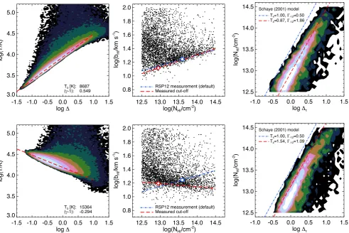
Measurements of thebHI–NHI cut-off obtained from two of our hydrodynamical simulations are displayed in Fig.1. The left-most
2Equation (5) ignores the weak dependence of the column density on the slope of theT–relation,NHI∝3/2−0.22(γ−1)T−
0.22
0,4 . Note also the nor-malization of this expression is 0.07 dex lower than equation (2) inRSP12. This difference is due to the slightly different cosmological parameters and case-A recombination coefficient, αHII=4.063×10⁻¹³T−
0.72 4 cm3s
−1 , assumed in this work.
panels display theT–relation in the simulations. The power-law relationship between the gas at the lower boundary of theT−
plane, shown by the red dashed lines, is estimated by finding the mode of the gas temperature in density bins of width 0.02 dex at log=0 and−0.75. The middle panels show the corresponding
bHI–NHI plane and the measured cut-off (red dashed lines). For comparison, theRSP12observational measurement is displayed by the blue dot–dashed lines;note this is shown in both of the middle panels and is not a fit to the simulation data.The simulation in the top panels has a maximally steepT–relation with (γ−1)=0.55, while the bottom panels display a model with an inverted T– relation, (γ −1)= −0.29. This qualitative comparison indicates that aT–relation which is inverted over 1012.5≤N
HI/[ cm−
2]≤
1014.5is indeed inconsistent with the Voigt profile fits to the KBSS
data, in agreement with the conclusion of RSP12. However, the value ofNHI,0in the simulations, indicated by the red diamond in
the middle panels, is∼0.65 dex smaller than the value used by RSP12, shown by the blue circle.
The explanation for this becomes apparent on examining the right-most panels in Fig.1, which display the relationship between
NHIand the corresponding optical depth-weighted overdensities at the line centres.3The blue dot–dashed lines display equation (5)
assumingT0, 4 =1 and−12 =0.5. The slope of this relation is
in excellent agreement with the simulation data, implying that a power-law relationship betweenandNHI, as inferred by Schaye
(2001), is a very good approximation.
On the other hand, the normalization of this relation disagrees with the simulations. Since the temperature dependence of equa-tion (5) is weak, this difference is mainly due to the low value of
−12 =0.5RSP12used to estimateNHI,0. This was based on the
results of Faucher-Gigu`ere et al. (2008), who inferred−12from the
Lyαforest opacity assuming an IGM temperature at mean density ofT0=2.1×10⁴K (Zaldarriaga et al.2001). As Faucher-Gigu`ere
et al. (2008) correctly point out, the Lyαforest opacity constrains the quantityT−0.72
0 / −12, and so assuming a larger (smaller) IGM
temperature4at mean density will translate their constraint into a
smaller (larger) value of−12if the Lyαopacity remains fixed. In
addition, Faucher-Gigu`ere et al. (2008) obtained their−12
mea-surements using an analytical model for IGM absorption which ignored the effect of redshift space distortions on the Lyαforest opacity. Including peculiar velocities and line broadening, as we do with our simulations, raises the−12required to match a given
value of the mean transmission in the Lyαforest by up to 30 per cent (Becker & Bolton2013). The Faucher-Gigu`ere et al. (2008) mea-surements are therefore systematically lower (by a factor of 2 or more) compared to the value we require to match our mock spectra to the mean transmission measurements of Becker et al. (2013) if
T0∼1×10⁴K.
3FollowingS99, we match the column densities measured with VPFIT to the optical depth weighted overdensity of the gas at the line centre,
τ = τii/τi, where the summation is over all pixels,i, along a simulated sight-line. This mitigates the effect of redshift space distortions arising from peculiar motions and line broadening, which would otherwise distort the direct mapping betweenNHIandin real space.
4The IGM temperature assumed by Faucher-Gigu`ere et al. (2008) is based on the results of Zaldarriaga et al. (2001), who inferredT0from the Lyα forest power spectrum after calibrating their measurement with a dark mat-ter only simulation performed with a (now) outdated cosmology. Since
τLyα∝T0−0.72/ −12, it is therefore not entirely coincidental that theRSP12 constraint onT0is similar to the measurement presented by Zaldarriaga et al. (2001).
at University of Nottingham on July 4, 2016
http://mnras.oxfordjournals.org/
Figure 1. Top left: contour plot of the volume weighted IGMT−plane in one of the hydrodynamical simulations used in this study. The number density of the data points increases by 0.5 dex with each contour level. The red dashed line displays the power-law approximation,T=T0γ−1, to theT–relation at log≤1. Top middle: the correspondingbHI−NHIplane for 4000 absorption features identified in mock Lyαforest spectra drawn from the simulation. The red dashed line corresponds to the measuredbHI−NHIcut-off, while the blue dot–dashed line shows the observational measurement presented byRSP12. The red diamond indicates the column density corresponding to gas with an optical depth weighted overdensity of logτ=0 in the simulation,NHI,0, and
the blue circle shows the value assumed byRSP12. Top right: contour plot ofNHIagainst the optical depth weighted gas overdensity at the line centres. The number density of data points increases by 0.25 dex within each contour level. The red dashed curve displays the analytical model of Schaye (2001), evaluated using the parameters adopted in the simulation. The blue dot–dashed line instead assumesT4=1 and−12=0.5. Bottom: as for the upper panels, but now for a simulation with an invertedT–relation. Note that the blue dot–dashed line in the middle panel again shows the observational measurement fromRSP12.
This is demonstrated by the red dashed lines in the right-hand panels of Fig. 1, which display equation (5) evaluated using the photo-ionization rates and gas temperatures used in the simula-tions. Although the agreement between the analytical model and simulations is still not perfect,5the higher
−12values result in a
significantly improved correspondence. We therefore conclude that the valueNHI,0=1013.6cm−2assumed byRSP12is biased high by ∼0.65 dex. As we will demonstrate, this bias translates into a signifi-cant overestimate ofT0. Finally, note that the 68 (95) per cent bounds
on the range of optical depth weighted overdensities probed by ab-sorption lines with column densities 1012.5≤N
HI/[ cm−
2]≤1014.5
are−0.2logτ 0.7 (−0.4logτ1.2) atz=2.4. The
bHI–NHIcut-off approach will be largely insensitive to the slope of theT–relation outside this range of overdensities.
3.2 A re-evaluation of the inferredT–relation atz =2.37
We now turn to the key result of this work, summarized in Fig.2, which displays the relationship betweenbHI,0–T0(upper panel) and
5Note thatand
τare slightly different quantities, and this comparison is thus not exact.
(γ −1)–(−1) (lower panel) obtained from the hydrodynamical simulations. Our choice ofNHI,0=1012.95cm−2corresponds to the
average value ofNHIassociated with gas with logτ=0 in all 18 simulations used in the analysis. In practice,NHI,0varies slightly
from one simulation to the next due to the weak dependence of the column density on the thermal state of the gas, ranging from 1012.8cm−2to 1013.1cm−2in our coldest to hottest simulations. We
found adopting values ofNHI,0 outside of this range introduces
an increasingly significant scatter into thebHI,0–T0correlation (see
also fig. 5 in Schaye et al.2000), invalidating the assumption that equation (4) is a single power law (i.e. thatζ1=0 holds) and biasing
any measurement ofT0if (γ −1)=0.
The dashed red lines in Fig. 2 display the best-fitting power laws to the simulation data given by equations (1) and (2), where
ζ2 = 1.46, ξ1 = 0.65 and ξ2 = 2.23 assuming ζ1 = 0 and
NHI,0=1012.95cm−2. The blue dot–dashed lines display the
ana-lytical relations used byRSP12. The dotted lines with shaded error regions show theRSP12measurements for two value ofNHI,0. The
grey bands correspond to the case where we have rescaled the de-faultRSP12bHI,0to the value measured atNHI=10
12.95cm−2. The
light blue band in the upper panel of Fig.2shows their original mea-surement assumingNHI,0=1013.6cm−2. The best-fittingbHI,0–T0
at University of Nottingham on July 4, 2016
http://mnras.oxfordjournals.org/
Figure 2. Measurements of the amplitudebHI,0 (upper panel) and slope (−1) (lower panel) of thebHI−NHIcut-off against the correspondingT0 and (γ−1) from 18 hydrodynamical simulations. The thick (thin) bootstrap error bars correspond to the 68 (95) per cent confidence intervals around the median. The red dashed lines give the maximum likelihood power-law fits to the data using the bootstrapped uncertainty distributions, while the blue dot– dashed lines display the analytical relations used byRSP12. The solid black lines show the power-law relationsS99inferred from their hydrodynamical simulations (note these are obtained atz=3 rather thanz=2.4), and the grey shaded bands display theRSP12default measurements. Note that the
RSP12measurement ofbHI,0has been rescaled to correspond toNHI,0= 1012.95cm−2; the light blue band gives the value measured byRSP12when assumingNHI,0=1013.6cm−2. The models C15Pand T15fast refer to two additional simulations which test the effect of cosmological parameters and Jeans smoothing (see text for details). These latter two models were not included in the maximum likelihood fits.
relation lies slightly above the result for pure thermal broadening, indicating that additional processes such as Jeans smoothing (which also scales asT1/2; see e.g. Gnedin & Hui1998) and Hubble
broad-ening impact on the minimum line width.
For comparison, the solid black lines display the relationship at
z=3 found from the simulations performed byS99. These authors inferred a similar slope for thebHI,0–T0relation, but with a
posi-tive offset of around∼0.1 dex relative to this work. Aside from the slightly lower redshift we consider here, there are several possible explanations for this result. The first is the smaller dynamic range of the hydrodynamical simulations used byS99, which employed a gas particle mass of 1.65×10⁶(
bh2/0.0125)(h/0.5)−3Mwithin a
box size of 2.5h−1Mpc and were performed with a modified version
of the smoothed particle hydrodynamics codeHYDRA(Couchman,
Thomas & Pearce1995). Additionally, the six simulationsS99 anal-ysed all used different assumptions for cosmological parameters and the IGM thermal history, which further complicates a direct com-parison. A final possibility is that there are differences in the version ofVPFITS99used to fit the absorption lines. The results presented by
S99already indicated that the assumption of purely thermal broad-ening may result in an overestimate of the gas temperature, but our analysis suggests that the factor by which the velocity widths of the
lines at thebHI−NHIcut-off are actually increased by non-thermal broadening is rather small.
The relatively good agreement of the slopes of the best fit and analytical relations in Fig.2reflects the fact that both equation (5) and the assumption thatbHI∝T
1/2at theb
HI−NHIcut-off capture the results of simulations quite accurately. Interestingly, however, although the slope of thebHI–T0 relation is similar to that found
byS99atz=3, we find a much steeper slope for the relationship between (−1) and (γ−1).S99concluded the weaker dependence they found between (−1) and (γ−1) would hamper any precise measurement of the slope of theT–relation. Our results instead suggest that atz∼2.4 the slope of thebHI–NHIcut-off is able to discriminate rather well between differingT–relations. We have checked that using the smaller line sample (300 lines, with 500 bootstrap resamples) used byS99increases the uncertainties on the cut-off measurements but does not change this conclusion. The exact explanation for this difference is again unclear, although we again speculate differences in the hydrodynamical simulations may play a role. However, the potentially greater sensitivity to (γ−1) provides additional motivation for revisitingbHI–NHIcut-off measurements at higher redshifts.
We have also verified that the best-fitting power-law relations in Fig.2should be robust to small differences in the assumed cos-mology and uncertainties in the pressure (Jeans) smoothing scale of gas in the IGM (see Rorai, Hennawi & White2013for a recent discussion). The circles showbHI,0and (−1) measured from an
additional simulation, C15P(see Becker & Bolton2013), which was
performed with cosmological parameters consistent with the Planck results, m =0.308, = 0.692,bh2 = 0.0222,h= 0.678,
σ8=0.829 andns=0.961 [Ade et al. (Planck Collaboration XVI)
2013]. The diamonds show the results obtained from the simulation T15fast described in Becker et al. (2011). This simulation rapidly heats the IGM fromz=3.5 to 3.0 by∼9000 K, in contrast to the more gradual heating used in our fiducial simulations. The good agreement of both these models with the best-fitting relations indi-cates that neither of these issues should be a significant concern in our analysis.
Combining these results with equations (3) and (4) and apply-ing them to the defaultRSP12measurement ofbHI,0and (−1),
we inferT0=[1.00−+00..3221]×104K and (γ −1)=0.54±0.11 at z =2.37 (cf.T0=[1.87±0.08]×104K andγ−1=0.47±0.10
fromRSP12). Note thatwe do not recompute theRSP12 statisti-cal uncertainty estimates; we instead simply rescale their published measurements ofbHI,0and (− 1) using the results of our
sim-ulations. We have, however, added (in quadrature) an additional systematic error to our measurement ofT0 by assuming an
un-certainty of±0.2 dex in log, the fractional overdensity corre-sponding to the column densityNHI,0at whichT0is measured (i.e.
log=0.0±0.2). This accounts for the intrinsic scatter in the relationship betweenNHIandτ in our simulations (see Fig.1) as well as the small uncertainty in the mean transmitted flux in the Lyα forest (Becker et al.2013).
Our recalibrated measurement for the slope of theT– rela-tion is fully consistent withRSP12. Importantly, however, we find their measurement ofT0is biased high by around 9000 K. This is
primarily due the value ofNHI,0=1013.6cm−2they adopt in their
analysis – this column density corresponds to gas with∼2–4 in our simulations – and to a smaller extent their assumption of pure thermal broadening at thebHI–NHI cut-off. Finally, we stress we did not reanalyse theRSP12observational data in this work. As a result we are unable to fully assess the importance of other potential systematics such as metal line contamination, spurious line fits or
at University of Nottingham on July 4, 2016
http://mnras.oxfordjournals.org/
[image:5.595.49.286.53.297.2]bias due to differences in the line fitting procedure (e.g. Rauch et al. 1993). Ideally, potential biases arising from the latter two possibil-ities should be minimized by applying exactly the same line profile fitting procedure to both the observationsandsimulations (e.g.S99; Bolton et al.2012).
3.3 Comparison to previous measurements
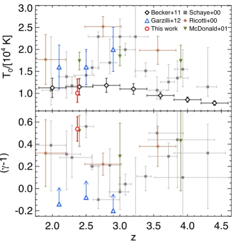
Our recalibrated measurements of the T– relation at z ∼ 2.4 are compared to previous measurements in Fig. 3. The T0 and
(γ−1) constraints obtained in this study are in excellent agreement with the recent, independent measurement presented by Becker et al. (2011) using the curvature statistic. These authors directly measure T( ¯)=[2.54±0.13]×104K (2σ) at a characteristic
overdensity of ¯=4.4 at z = 2.4. The T0 and (γ − 1)
re-sults rederived here from the RSP12data translate to a value of
T( ¯)=[2.22+0.80
−0.59]×10
4K (1σ), which is fully consistent with
the Becker et al. (2011) value. Alternatively, translating the Becker et al. (2011)T( ¯) measurement to a temperature at the mean density assuming (γ−1)=0.54±0.11 yieldsT0=[1.15±0.19]×104K
(1σ). For the value of (γ −1) measured here, therefore, both the Becker et al. (2011) measurements and the present results are con-sistent with a value ofT0near 1×10⁴K atz=2.4. Note that Becker
et al. (2011) also strongly constrainT0to be relatively low atz >
4, where the characteristic overdensity probed by the curvature ap-proaches the mean density. For example, atz=4.4 they findT0to be
in the range 0.70–0.94×10⁴K (2σ) for (γ−1)=1.3–1.5. This
im-plies only a moderate boost to the IGM temperature at mean density during HeIIreionization, although the precise evolution ofT0over
Figure 3. A comparison of the temperature at mean density,T0(top panel), and slope of theT–relation, (γ−1) (bottom panel), inferred in this work (red circles) to other recent constraints obtained using a variety of different methods at 2≤z≤4.5. These are: the curvature statistic from Becker et al. (2011) (black diamonds); the wavelet amplitude PDF from Garzilli et al. (2012) (blue triangles), and thebHI−NHIcut-off analyses presented by Schaye et al. (2000) (grey squares), Ricotti et al. (2000) (orange diamonds) and McDonald et al. (2001) (inverted green triangles). All uncertainties are 1σ. TheT0values inferred from the measurements of Becker et al. (2011) assume (γ−1)=0.54±0.11, i.e. the value inferred in this work atz=2.4.
2.4< z <4.4 will depend on the evolution of (γ −1) over these redshifts.
Our measurement of T0 is also in reasonable agreement with
those of Garzilli et al. (2012), who performed an analysis of the wavelet amplitude PDF (see also Lidz et al. 2010), obtain-ingT0=[1.6±0.4]×104K (1σ) at the slightly higher redshift
ofz=2.5. We are also consistent with the earlierbHI–NHI mea-surements obtained by Schaye et al. (2000) atz=2.4; as already discussed these authors used a similar technique but smaller data set compared toRSP12. We are unable to directly compare thebHI–
NHImeasurements from Ricotti et al. (2000) to our measurement, since these authors do not present results at z= 2.4. However, they find a significantly larger value ofT0=25200±2300 K at
z=2.75, which would require aT–relation slope of (γ−1)∼1 for consistency with the Becker et al. (2011) measurements at the same redshift. Finally, McDonald et al. (2001), again using the
bHI–NHIcut-off (although with a different method to Schaye et al. 2000), inferT =2.26±0.19×10⁴K at= 1.66± 0.11.
Al-though these authors do not present a measurement ofT0, using
their measurement of (γ −1)=0.52±0.14 this corresponds to
T0=1.74±0.20×10⁴K. This temperature is somewhat higher
than the three other measurements atz= 2.4, by 2–3σ. Despite this, however, there appears to be a reasonable consensus on the thermal state of the low-density IGM atz∼2.4 from both Lyα transmission statisticsandline decomposition analyses.
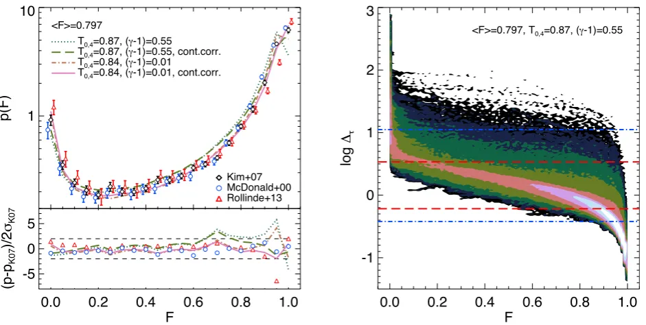
On the other hand, while our revised value of (γ − 1) = 0.54 ± 0.11 is fully consistent with the original line decomposition analyses of Schaye et al. (2000) and McDonald et al. (2001) and the lower limits from the wavelet PDF obtained by Garzilli et al. (2012), as noted byRSP12 there appears to be some tension with constraints based on the observed transmission PDF (Kim et al.2007, hereafterK07) which appear to favour an isothermal or perhaps even inverted T–relation at 2 < z <3 (Bolton et al.2008; Viel et al.2009). In the left hand panel of Fig. 4we revisit this by comparing the PDF of the transmitted flux from two of our hydrodynamical simulations to three obser-vational measurements of the Lyαforest transmission PDF from high-resolution (R∼40 000) data atz 2.4–2.5 (K07; McDonald et al. 2000; Rollinde et al.2013). The mock spectra have been drawn from models with aT–relation with either (γ−1)=0.55 or (γ − 1)= 0.01 at z= 2.553, and have aT0 value close to
the revised measurement obtained in this work. The spectra have been processed following a similar procedure to that outlined in Section 2.1, with two key differences. First, the spectra are scaled to match the mean transmission of theK07PDF data,F =0.797 at
z =2.52, and Gaussian distributed noise matching the variances,
σF, in each bin of theK07PDF is added. Secondly, for each model
we also implement an iterative continuum correction to the spectra to mimic the effect of a possible continuum placement error on the K07data. We first compute the median transmitted flux in each of our mock sight-lines and then deselect all pixels below 1σFof
this value. This procedure is then repeated for the remaining pixels until convergence is achieved. The final median flux is selected as the new continuum level.
The comparison in Fig. 4 demonstrates a T– relation with (γ − 1) = 0.55 is inconsistent with the K07 data at 4–7σ at 0.6 < F < 0.8, even when accounting for possible continuum misplacement (although see the analysis presented by Lee 2012 using an analytical model for the transmission PDF). An isothermal model on the other hand is in within 1–3σ of theK07data over the same interval. This is fully consistent with the more detailed analysis performed by Viel et al. (2009) and Bolton et al. (2008).
at University of Nottingham on July 4, 2016
http://mnras.oxfordjournals.org/
[image:6.595.46.283.381.626.2]Figure 4. Top left: the probability distribution of the transmitted flux (PDF) atz∼2.5. The observational data are fromK07atz =2.52, Rollinde et al. (2013) atz =2.5 and McDonald et al. (2000) atz =2.4. The data points from the latter two studies have been offset byF= ±0.0125 for clarity of presentation. The curves display the PDF obtained from two different hydrodynamical simulations of the Lyαforest atz=2.553 which assume aT–relation with either (γ−1)=0.55 or (γ−1)=0.01. Each of these models is furthermore shown with and without an estimate for the continuum correction (see text for details). Bottom left: the difference between the mock data and observations from Rollinde et al. (2013) and McDonald et al. (2000) with respect toK07, normalized by twice the 1σK07jack-knife errors. This accounts for a possible factor of 2 underestimate in the sample variance suggested by Rollinde et al. (2013). The horizontal dashed lines display the 2σ bound for these increased error estimates. Right: contour plot of the optical depth weighted overdensity against the transmitted flux in each pixel of the mock spectra drawn from the simulation withT0, 4=0.87 and (γ−1)=0.55. The number density of pixels increases by 0.5 dex within each contour level. The horizontal red dashed (blue dot–dashed) lines bound 68 (95) per cent of the overdensities corresponding to absorption lines with 1012.5≤NHI/[cm−
2]≤1014.5.
Note, however, that Rollinde et al. (2013) recently argued that the error bars quoted on theK07PDF measurements may be larger by up to a factor of 2 simply due to sample variance; these authors demonstrated the bootstrap or jack-knife errors on the data will be underestimated if the chunk size which the spectra are sampled over is too small. Comparison of the three observational measurements in Fig.4likewise suggests that the errors on the PDF measurements have been initially underestimated.
The lower panel in Fig.4therefore displays the difference be-tween theK07 PDF and the mock data and observations from Rollinde et al. (2013) and McDonald et al. (2000), divided through bytwicethe 1σjack-knife errors reported byK07. With these larger uncertainties the discrepancy with the (γ −1)=0.55 model de-creases, although the difference between the simulation and data is still∼2–3σ at 0.6< F<0.8 after accounting for a plausible continuum placement error. This is in reasonable agreement with Rollinde et al. (2013), who also reproduce theK07PDF atz=2.5 to within 2–3σ of the expected dispersion6estimated from mock
spectra drawn from the GIMIC simulation suite (Crain et al.2009) assuming (γ −1)∼0.35 andF =0.770. Rollinde et al. (2013) conclude there is no evidence for a significant departure from a
6This excludes the Rollinde et al. (2013)z=2.5 PDF bin atF=0.95, which is discrepant withK07at∼6σ even after doubling the K071σ error bars. Rollinde et al. (2013) attribute large differences atF>0.7 to continuum uncertainties, although our analysis suggests that a reasonable estimate for the continuum misplacement may still not fully explain this offset atF=0.95.
power-lawT–relation with (γ−1)>0. The remaining disagree-ment between the observations and a model with (γ −1)=0.55 suggests that increased errors due to continuum placement and sam-ple variance may still not fully account for the true uncertainties on the observational data.
In this context, it is worth stressing that the transmission PDF and
bHI−NHIcut-off are sensitive to a different range of IGM gas den-sities and hence also temperatures. The right-hand panel of Fig.4 displays the relationship between the optical depth weighted over-density and transmitted flux in each pixel of the spectra drawn from the simulation with (γ−1)=0.55, shown in the left panel. For com-parison, the red dashed (blue dot–dashed) lines bound 68 (95) per cent of the overdensities probed corresponding to absorption lines with 1012.5≤N
HI/[cm−
2]≤1014.5(i.e. the range used to measure
the bHI–NHI cut-off atz ∼ 2.4). Interestingly, the largest differ-ences between models and observations of the PDF arise almost exclusively in the underdense regions which are not well sampled by thebHI–NHIcut-off measurements. Furthermore, note that the
bHI–NHIcut-off is only sensitive to the coldest gas lying along the lower bound of theT−plane (e.g.S99). It therefore remains possible that a more complicated, multiple valued T − plane with significant scatter and/or a separate hot IGM component con-fined to the most underdense regions, logτ ∼ −0.5, may also influence the shape of the PDF atF>0.7. Indeed, recent radiative transfer simulations of HeIIreionization predict significant scatter
or even bimodality in theT−plane atz∼3 (Meiksin & Tittley 2012; Compostella et al.2013). More detailed studies of both the PDF and thebHI–NHIdistribution over a wider redshift range, com-bined with simulations which have increased dynamic range and/or
at University of Nottingham on July 4, 2016
http://mnras.oxfordjournals.org/
incorporate radiative transfer effects, will therefore be required to establish the importance of these effects.
4 C O N C L U S I O N S
We have performed a careful calibration of the measurement of theT–relation in the low-density IGM atz∼2.4. Our analysis is based on the bHI–NHI cut-off measured from mock Lyαforest spectra drawn from an extensive set of high-resolution hydrody-namical simulations, combined with accurate measurements of the mean transmitted flux in the Lyαforest (Becker et al.2013) and the KBSS line profile fits fromRSP12. We confirm the high value of the power-law slope, (γ−1), atz∼2.4 advocated byRSP12, but find a value for the temperature at mean density,T0, which is smaller
by almost a factor of 2. The latter is mainly due to a difference of 0.65 dex in the calibration of theNHI–correlation. The lower
in-ferred value for the temperature brings the measurement ofRSP12 into excellent agreement with the Becker et al. (2011) constraint on the IGM temperature at the same redshift, but inferred at somewhat higher gas density using the curvature distribution of the transmit-ted flux. More generally, recent IGM temperature measurements appear to now show reasonable agreement and to favour the lower end of the range of previously discussed values, suggesting that the heat injection into the IGM during HeIIreionization was moderate.
However, the high value of (γ −1) which now appears to have been measured with reasonable accuracy from thebHI–NHI distri-bution atz∼2.4 disagrees with that inferred from the transmitted flux PDF at z ∼ 2.5 (at 2–3σ for 0.6 < F < 0.8) even if as-suming (i) previously reported uncertainties on the PDF have been underestimated by a factor of 2 and(ii) a plausible estimate for the continuum placement uncertainty (see also Lee2012; Rollinde et al.2013). While it is possible this difference is due to system-atic uncertainties which remain underestimated, it is important to emphasize that thebHI–NHIdistribution and PDF are sensitive to the temperature of the IGM in nearly disjunct density ranges, with the PDF largely probing densities below the mean. While it appears very likely the IGMT–relation is not inverted during HeII reion-ization from both an observational and theoretical perspective (e.g. McQuinn et al.2009; Bolton, Oh & Furlanetto2009), it may be too early to completely discard the interesting possibility that our understanding of the heating of the highly underdense IGM is still incomplete.
The convergence towards a self-consistent set of parameters de-scribing the T–relation at z 2.4 represents an encouraging step towards establishing the detailed thermal history of the high-redshift IGM. The extension of the measurements based on the
bHI–NHIdistribution to a wider redshift range, and the development of methods that can push the temperature measurements to lower density and search for the predicted scatter or even bimodality in the
T−plane during HeIIreionization (e.g. Meiksin & Tittley2012;
Compostella et al.2013) will hopefully lead to a fuller characteriza-tion of the thermal state of the IGM and its evolucharacteriza-tion, and thus more generally to the properties of ionizing sources in the early Universe.
AC K N OW L E D G E M E N T S
The hydrodynamical simulations used in this work were performed using the Darwin Supercomputer of the Uni-versity of Cambridge High Performance Computing Service (http://www.hpc.cam.ac.uk/), provided by Dell Inc. using Strate-gic Research Infrastructure Funding from the Higher Education
Funding Council for England. We thank Volker Springel for mak-ing GADGET-3 available, Bob Carswell for advice on VPFIT and
the anonymous referee for a report which helped improve this pa-per. The contour plots presented in this work use the cube helix colour scheme introduced by Green (2011). JSB acknowledges the support of a Royal Society University Research Fellowship. GDB acknowledges support from the Kavli Foundation. MGH acknowl-edges support from the FP7 ERC Grant Emergence-320596. MV is supported by the FP7 ERC grant ‘cosmoIGM’ and the INFN/PD51 grant.
R E F E R E N C E S
Ade P. A. R. et al. (Planck Collaboration XVI), 2013, A&A, preprint (arXiv:1303.5076)
Becker G. D., Bolton J. S., 2013, MNRAS, 436, 1023
Becker G. D., Bolton J. S., Haehnelt M. G., Sargent W. L. W., 2011, MNRAS, 410, 1096
Becker G. D., Hewett P. C., Worseck G., Prochaska J. X., 2013, MNRAS, 430, 2067
Bolton J., Meiksin A., White M., 2004, MNRAS, 348, L43
Bolton J. S., Viel M., Kim T.-S., Haehnelt M. G., Carswell R. F., 2008, MNRAS, 386, 1131
Bolton J. S., Oh S. P., Furlanetto S. R., 2009, MNRAS, 395, 736
Bolton J. S., Becker G. D., Wyithe J. S. B., Haehnelt M. G., Sargent W. L. W., 2010, MNRAS, 406, 612
Bolton J. S., Becker G. D., Raskutti S., Wyithe J. S. B., Haehnelt M. G., Sargent W. L. W., 2012, MNRAS, 419, 2880
Bryan G. L., Machacek M. E., 2000, ApJ, 534, 57
Cen R., McDonald P., Trac H., Loeb A., 2009, ApJ, 706, L164 Compostella M., Cantalupo S., Porciani C., 2013, MNRAS, 435, 3169 Couchman H. M. P., Thomas P. A., Pearce F. R., 1995, ApJ, 452, 797 Crain R. A. et al., 2009, MNRAS, 399, 1773
Faucher-Gigu`ere C.-A., Lidz A., Hernquist L., Zaldarriaga M., 2008, ApJ, 688, 85
Furlanetto S. R., Oh S. P., 2009, ApJ, 701, 94
Garzilli A., Bolton J. S., Kim T.-S., Leach S., Viel M., 2012, MNRAS, 424, 1723
Gnedin N. Y., Hui L., 1998, MNRAS, 296, 44 Green D. A., 2011, Bull. Astron. Soc. India, 39, 289 Haehnelt M. G., Steinmetz M., 1998, MNRAS, 298, L21 Hui L., Gnedin N. Y., 1997, MNRAS, 292, 27
Hui L., Haiman Z., 2003, ApJ, 596, 9
Kim T.-S., Bolton J. S., Viel M., Haehnelt M. G., Carswell R. F., 2007, MNRAS, 382, 1657 (K07)
Lee K.-G., 2012, ApJ, 753, 136
Lidz A., Faucher-Gigu`ere C.-A., Dall’Aglio A., McQuinn M., Fechner C., Zaldarriaga M., Hernquist L., Dutta S., 2010, ApJ, 718, 199
McDonald P., Miralda-Escud´e J., Rauch M., Sargent W. L. W., Barlow T. A., Cen R., Ostriker J. P., 2000, ApJ, 543, 1
McDonald P., Miralda-Escud´e J., Rauch M., Sargent W. L. W., Barlow T. A., Cen R., 2001, ApJ, 562, 52
McQuinn M., Lidz A., Zaldarriaga M., Hernquist L., Hopkins P. F., Dutta S., Faucher-Gigu`ere C.-A., 2009, ApJ, 694, 842
Meiksin A., Tittley E. R., 2012, MNRAS, 423, 7 Miniati F., Elyiv A., 2013, ApJ, 770, 54
Miralda-Escud´e J., Rees M. J., 1994, MNRAS, 266, 343
Puchwein E., Pfrommer C., Springel V., Broderick A. E., Chang P., 2012, MNRAS, 423, 149
Raskutti S., Bolton J. S., Wyithe J. S. B., Becker G. D., 2012, MNRAS, 421, 1969
Rauch M., Carswell R. F., Webb J. K., Weymann R. J., 1993, MNRAS, 260, 589
Ricotti M., Gnedin N. Y., Shull J. M., 2000, ApJ, 534, 41
Rollinde E., Theuns T., Schaye J., Pˆaris I., Petitjean P., 2013, MNRAS, 428, 540
at University of Nottingham on July 4, 2016
http://mnras.oxfordjournals.org/
Rorai A., Hennawi J. F., White M., 2013, ApJ, 775, 81
Rudie G. C., Steidel C. C., Pettini M., 2012a, ApJ, 757, L30 (RSP12) Rudie G. C. et al., 2012b, ApJ, 750, 67
Schaye J., 2001, ApJ, 559, 507
Schaye J., Theuns T., Leonard A., Efstathiou G., 1999, MNRAS, 310, 57 (S99)
Schaye J., Theuns T., Rauch M., Efstathiou G., Sargent W. L. W., 2000, MNRAS, 318, 817
Shull J. M., France K., Danforth C. W., Smith B., Tumlinson J., 2010, ApJ, 722, 1312
Springel V., 2005, MNRAS, 364, 1105
Syphers D., Anderson S. F., Zheng W., Meiksin A., Haggard D., Schneider D. P., York D. G., 2011, ApJ, 726, 111
Theuns T., Leonard A., Efstathiou G., Pearce F. R., Thomas P. A., 1998, MNRAS, 301, 478
Theuns T., Schaye J., Zaroubi S., Kim T., Tzanavaris P., Carswell B., 2002a, ApJ, 567, L103
Theuns T., Zaroubi S., Kim T.-S., Tzanavaris P., Carswell R. F., 2002b, MNRAS, 332, 367
Viel M., Bolton J. S., Haehnelt M. G., 2009, MNRAS, 399, L39 Worseck G. et al., 2011, ApJ, 733, L24
Zaldarriaga M., Hui L., Tegmark M., 2001, ApJ, 557, 519
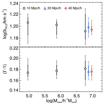
A P P E N D I X A : C O N V E R G E N C E T E S T
In Fig.A1we present a convergence test of our results by applying thebHI−NHIcut-off algorithm to five simulations with different box sizes and gas particle masses. One of the simulations corre-sponds to the fiducial box size (10h−1Mpc) and gas particle mass
resolution (Mgas=9.2×10⁴h−1M) used in this work. Two further
models test the mass resolution within a 10h−1Mpc box, assuming
Mgas = 7.4×10⁵h−1M and 5.9×10⁶h−1M, respectively.
The final two models test convergence with simulation volume, and have a fixed gas particle mass ofMgas=5.9×10⁶h−1Mwithin
20h−1Mpc and 40h−1Mpc boxes. These five simulations are also
described in Becker et al. (2011), and correspond to models C15 and R1–R4 in their table 2.
Mock spectra extracted atz= 2.355 were analysed using the procedure described in Section 2 using a sample of 4000 lines, with uncertainties onbHI,0 and ( − 1) estimated by bootstrap
[image:9.595.318.537.55.273.2]sam-pling with replacement 4000 times. The measurements of bHI,0
Figure A1. The amplitude, bHI,0 (top panel), and slope, (− 1) (bot-tom panel) of thebHI−NHIcut-off measured from simulations with ei-ther a fixed box size (10h−1Mpc, black circles) or fixed mass resolution (Mgas=5.9×10⁶h−1M) using a sample of 4000 Lyαabsorption lines. For clarity of presentation the blue triangles and red diamonds have been offset in logMgasby 0.1 and 0.2 dex, respectively. The thick (thin) bootstrap error bars correspond to the 68 (95) per cent confidence intervals around the median. The fiducial box size and mass resolution used in this work are 10h−1Mpc andMgas=9.2×10⁴h−1M.
and ( − 1) are consistent within the 68 per cent bootstrapped confidence intervals around the median, indicating that our results should be well converged with box size and mass resolution. We have further verified that a smaller sample of 300 lines (e.g.S99) significantly increases the bootstrapped uncertainties but does not introduce a systematic offset to the results.
This paper has been typeset from a TEX/LATEX file prepared by the author.
at University of Nottingham on July 4, 2016
http://mnras.oxfordjournals.org/