Advance Access publication on ?? ???? 20??
C
20?? Biometrika Trust Printed in Great Britain
Going off grid: Computationally efficient inference for
log-Gaussian Cox processes
BY D. SIMPSON
Department of Mathematical Sciences, University of Bath, Bath BA2 7AY, U.K.
J. B. ILLIAN
Centre for Research into Ecological and Environmental Modelling, University of St Andrews, St Andrews, Fife KY16 9LZ, U.K.
Department of Mathematical Sciences, Norwegian University of Science and Technology,
N-7491 Trondheim, Norway. 10
F. LINDGREN
Department of Mathematical Sciences, University of Bath, Bath BA2 7AY, U.K. [email protected]
S. H. SØRBYE 15
Department of Mathematics and Statistics, UiT The Arctic University of Norway, N-9037 Tromsø, Norway
ANDH. RUE
Department of Mathematical Sciences, Norwegian University of Science and Technology, 20
N-7491 Trondheim, Norway [email protected]
SUMMARY
This paper introduces a new method for performing computational inference on log-Gaussian Cox processes. The likelihood is approximated directly by making novel use of a continuously 25
specified Gaussian random field. We show that for sufficiently smooth Gaussian random field prior distributions, the approximation can converge with arbitrarily high order, while an ap-proximation based on a counting process on a partition of the domain only achieves first-order convergence. The given results improve on the general theory of convergence of the stochastic partial differential equation models, introduced by Lindgren et al. (2011). The new method is 30
demonstrated on a standard point pattern data set and two interesting extensions to the classi-cal log-Gaussian Cox process framework are discussed. The first extension considers variable sampling effort throughout the observation window and implements the method of Chakraborty et al. (2011). The second extension constructs a log-Gaussian Cox process on the world’s oceans. The analysis is performed using integrated nested Laplace approximation for fast approximate 35
Some key words: Approximation of Gaussian random fields; Gaussian Markov random fields; Integrated nested Laplace approximation; Spatial point processes; Stochastic partial differential equations.
1. INTRODUCTION
Data consisting of sets of locations at which some objects are present are common in biology,
40
ecology and economics. The appropriate statistical models for this type of data are spatial point process models, which have been extensively studied by statisticians and probabilists (Møller & Waagepetersen, 2004; Illian et al., 2008) but are less commonly used by the scientists producing the data sets. Point process models are often hard to fit, so scientists often resort to using inappro-priate methods. (Chakraborty et al., 2011) discuss this in the context of presence-only datasets,
45
and outline various ad hoc approaches used by ecologistsThere is an interesting discussion of this in the context of presence only data sets (Chakraborty et al., 2011), which outlines a number of ad hoc approaches taken by the ecological community.
Many real data sets do not have the simple structure usually considered in the classical sta-tistical literature, i.e., that of a simple point pattern that has been observed everywhere within a
50
simple, often rectangular, plot. For instance, in real data sets the observation process is often not straightforward due to practical limitations, or the observation window is complex. This includes data sets mapping the locations of bird species, for which very little data have been collected in the Himalayas for obvious reasons. Therefore, on top of sampling issues such as incompletely observed point patterns, positional errors, etc., this data set has a large hole where it is believed
55
that birds reside, but it is impractical to look for them. Very different, but similarly complex, data deal with freak waves in the oceans. Even if we ignore temporal aspects, or the uncertainty in the observed locations, this data set remains complicated, as the observation window covers most of a sphere and has a very complicated boundary. Motivated by data sets of this nature, this paper proposes an easy to use, computationally efficient method for performing inference on spatial
60
point process models that is sufficiently flexible to handle these and other data structures. In this paper we focus on log-Gaussian Cox processes, a class of flexible models that is par-ticularly useful in the context of modelling aggregation relative to some underlying unobserved environmental field (Møller et al., 1998; Illian et al., 2012). However, standard methods for fit-ting Cox processes are computationally expensive and the Markov chain Monte Carlo methods
65
that are commonly used are difficult to tune for this problem. Recently, Illian et al. (2012) de-veloped a fast, flexible framework for fitting log-Gaussian Cox processes using integrated nested Laplace approximation (Rue et al., 2009). They construct a Poisson approximation to the true log-Gaussian Cox process likelihood to perform inference on a regular lattice over the observa-tion window, counting the number of points in each cell. If the lattice is fine enough and the
la-70
tent Gaussian field is appropriately discretised, this approximation is quite good (Waagepetersen, 2004), but it can be computationally wasteful, especially when the process intensity is high or the observation window is large or oddly shaped. New results on the strong convergence of the lattice approximation, provided in the Appendix, show that the rate of convergence on a p×p
lattice is fundamentally limited toO(p−1)by the counting approximation.
75
In the Appendix, we provide detailed results on the convergence of the approximations pro-posed in this paper. In particular, we show that, for a Gaussian random field with fixed param-eters, the posterior distributions generated using the proposed method will converge strongly to the true posterior distribution. Furthermore, it is shown that these posterior distributions can converge with arbitrarily high order and the convergence is limited only by the smoothness of
80
significantly improve the existing convergence theory for these models. In particular, we show that the approximate posterior distributions converge weakly and the error when computing a
posterior functional is almostO(h−1). 85
The first of our aims is to re-examine the standard methodology for Bayesian inference on log-Gaussian Cox processes and to propose an approach that is much more computationally efficient based on continuously specified finite-dimensional Gaussian random fields. The key characteris-tic of our approach is that the specification of the Gaussian random field is completely separated from the approximation of the likelihood, leading to far greater flexibility. The second aim is to 90
demonstrate that this approach can be handled within the general approximation framework of Rue et al. (2009), by modelling the Gaussian random field through a stochastic partial differen-tial equation (Lindgren et al., 2011). This provides a unified modelling structure. An associated
R-package makes our methods that accessible to scientists.
2. LOG-GAUSSIANCOX PROCESSES 95
Consider a bounded region Ω⊂R2. A simple point process model is the inhomogeneous
Poisson process, in which the number of points within a region D⊂Ωis Poisson distributed with meanΛ(D) =RDλ(s)ds, whereλ(s)is the intensity surface of the point process. Given the intensity surface and a point patternY,the likelihood of an inhomogeneous Poisson process
is 100
π(Y |λ) = exp
|Ω| −
Z
Ω
λ(s)ds
Y
si∈Y
λ(si). (1)
This likelihood is analytically intractable, as it requires the integral of the intensity function, which typically cannot be calculated explicitly. This integral can, however, be computed numer-ically using standard methods.
Treating the intensity surface as a realisation of a random fieldλ(s)yields a particularly flex-ible class of point processes known as Cox or doubly stochastic Poisson processes (Møller & 105
Waagepetersen, 2004). These are typically used to model aggregation in point patterns resulting from observed or unobserved environmental variation. In this paper we consider log-Gaussian Cox processes, where the intensity surface is modelled aslogλ(s) =Z(s), andZ(s)is a Gaus-sian random field. Conditional on a realisation of Z(s), a log-Gaussian Cox process is an in-homogeneous Poisson process. The likelihood for such a process is of the form (1), where the 110
integral is further complicated by the stochastic nature ofλ(s), and methods for approximating (1) are the focus of the next two sections. Log-Gaussian Cox processes fit naturally within the Bayesian hierarchical modelling framework and are latent Gaussian models. They may be fitted using the integrated nested Laplace approximation approach of Rue et al. (2009), allowing us to construct models that include covariates, marks and non-standard observation processes while 115
still allowing computationally efficient inference (Illian et al., 2012). Therefore, approximating the likelihood in (1) constitutes a basic calculation for practical problems such as those discussed in Section 7.
3. COMPUTATION ON FINE LATTICES IS WASTEFUL
A common method for performing inference with log-Gaussian Cox processes is to take the 120
observation windowΩ, construct a fine regular lattice over it, and then consider the number of pointsNij observed in each cellsij of the lattice (Møller et al., 1998; Illian et al., 2012). It is a
consid-ered as independent Poisson random variables, that isNij ∼Po(Λij),whereΛij =
R
sijλ(s)ds
is the total intensity in each cell. It is impossible to compute the total intensity for each cell and
125
we therefore use the approximationΛij ≈ |sij|exp(zij), wherezij is a representative value of
Z(s)within the cellsij and|sij|is the area of cellsij. The log-Gaussian Cox process model can
then be treated within the generalised linear mixed model framework. This method has been used in a number of applications and converges to the true solution as the size of the cells decreases to zero; see Corollary A1 or Waagepetersen (2004).
130
The computational challenge is that, ifZ(s)is a general Gaussian random field, the multivari-ate Gaussian vectorz that contains thezijs will have a dense covariance matrix. The resulting
computational complexity limits this method to quite small lattices. If Z(s) is stationary and the observation window is a rectangle, it is possible to use the block Toeplitz structure of the covariance matrix to speed up some computations (Møller et al., 1998). Unfortunately, the block
135
Toeplitz structure is fragile and any inference method that constructs a second-order approx-imation to the posterior distribution, such as manifold Markov chain Monte Carlo simulation (Girolami & Calderhead, 2011) or the integrated nested Laplace approximation, will destroy the computational savings.
A common computationally efficient approach is to modelz as a conditional autoregressive
140
model on the fine lattice and use this to perform fast computations (Rue & Held, 2005). The conditional autoregressive approach has been used extensively in applications and may be fitted using the integrated nested Laplace approximation (Illian et al., 2012). Both methods rely heavily on the regularity of the lattice, as it is quite difficult to construct a conditional autoregressive model on an irregular lattice that is resolution-consistent (Rue & Held, 2005).
145
However, these methods are unsatisfactory since the computational lattice has two fundamen-tally different roles. The first and most natural role is to approximate the latent Gaussian random fieldZ(s). The second and rather unnatural role of the computational lattice is to approximate the locations of the points, even though the data have often been collected with high precision. Clearly, the finer the lattice is, the less information is lost, so the quality of the likelihood
approx-150
imation primarily depends on the size of the grid. In fact, Corollary A1 shows that this binning process is the dominant source of error in the lattice approximation. As a result, we are required to compute on a much finer grid than is necessary for the approximation of the latent Gaussian field, making lattice-based approaches inherently wasteful in this context.
The inflexibility inherent in lattice-based methods also implies that the approximation to the
155
latent random field cannot be locally refined. In the problem considered in Section 7·3, a large region has not been sampled. Generating a high resolution approximation to the latent field over this area would be computationally wasteful. It would be more efficient to reduce the resolution in these areas without affecting that in those that have been sampled. While this is impossible with lattice-based methods, the flexible method introduced here allows local changes to the resolution
160
of the approximation.
4. APPROXIMATING THE LIKELIHOOD USING A FINITE-DIMENSIONAL RANDOM FIELD Rather than defining a Gaussian random field over a fine lattice, we propose a finite-dimensional continuously specified random field of the form
Z(s) =
n
X
i=1
wherez= (z1, . . . , zn)T is a multivariate Gaussian random vector and{φi(s)}ni=1is a set of lin- 165
early independent deterministic basis functions. This is similar in spirit to the Karhunen–Lo`eve decomposition of stochastic processes, which is based on eigen-decomposition of the covariance function of the process. Three other common approximations to Gaussian random fields can also be expressed as in (2). Process convolution models (Higdon, 1998) use the approximation
Z(s) =R
Ωk(s, s
0)dW(s0)≈PN
i=1zik(s, si),where the first integral is a white noise integral, 170
thezi are independent Gaussian random variables, and the points si lie on a lattice withinD.
The second class of models uses correlated weightszand selects basis functions, either based on a parent Gaussian process as for predictive processes (Banerjee et al., 2008), or from other con-siderations, as in fixed-rank kriging (Cressie & Johannesson, 2008). Chakraborty et al. (2011) investigated log-Gaussian Cox process models using predictive processes. The third class com- 175
prises the stochastic partial differential equation models of Lindgren et al. (2011), which take
φi(s)to be compactly-supported piecewise linear functions. This choice ofφi(s)delivers
con-siderable computational benefits and will be further explored in Section 5 and Appendix A·4. All of the examples in this paper use stochastic partial differential equation models for the latent
processZ(s). 180
With the continuous Gaussian random field model in place, we are in a position to attack the intractable likelihood (1). In this section, we outline a procedure for approximating the likelihood that extends the standard approximation to the non-lattice, unbinned data case. The log-likelihoodlogπ(y|Z) =|Ω| −R
Ωexp{Z(s)}ds+
PN
i=1Z(si)consists of two terms: the
stochastic integral, and the evaluation of the field at the data points. While the continuously- 185
specified stochastic partial differential equation models allow us to compute the sum term ex-actly, we must approximate the integral by a sum. Consider a deterministic integration rule of the general formR
Ωf(s)ds≈
Pp
i=1α˜if(˜si),for fixed, deterministic nodes{˜si}pi=1and weights
{α˜i}pi=1. Using this integration rule, we can construct the approximation
log{π(y |z)} ≈C− p
X
i=1
˜
αiexp
n
X
j=1
zjφj(˜si)
+
N
X
i=1
n
X
j=1
zjφj(si)
=C−α˜Texp(A1z) + 1TA2z, (3)
whereC is a constant,[A1]ij =φj(˜si)is a matrix containing the values of the latent Gaussian 190
model (2) at the integration nodes{s˜i}, and[A2]ij =φj(si)evaluates the latent Gaussian field
at the observed points{si}.
The advantage of the approximation (3) is that it is of Poisson form. In particular, given z
andθ, the approximate likelihood consists ofN +pindependent Poisson random variables. To see this, we writelogη = (zTAT1, zTAT2)T andα= ( ˜αT,0TN×1)T. Then, if we construct some 195
pseudo-observationsy= (0Tp×1,1TN×1)T, the approximate likelihood factors as
π(y|z)≈C
N+p
Y
i=1
ηyi
i e
−αiηi, (4)
which is similar to the likelihood for observingN +pconditionally independent Poisson random variables with meansαiηi and observed valuesyi.
Numerical integration schemes that lead to likelihood approximations of the form (4) were 200
to log-Gaussian Cox processes, probably due to the paucity of computationally efficient contin-uously specified Gaussian random field models.
In the Appendix, we show that the approximate posterior distribution converges to the true
205
posterior distribution generated using the correct log-Gaussian Cox process likelihood at a rate that depends on the smoothness of the field and the quality of the integration rule. Hence, while Baddeley & Turner (2000) suggest placing “one [...] point, either systematically or randomly”, for log-Gaussian Cox processes, there is a strong advantage to carefully designing the underlying integration scheme.
210
5. STOCHASTIC PARTIAL DIFFERENTIAL EQUATIONS ANDMARKOV RANDOM FIELDS The approximation outlined in Section 4 will work for any finite-dimensional random field (2). This section shows how this approach fits naturally with our preferred finite-dimensional random field model. In particular, we review the stochastic partial differential equation construc-tion of Lindgren et al. (2011) and show how this naturally extends the condiconstruc-tional autoregressive
215
modelling strategy of Illian et al. (2012).
The basic idea of Lindgren et al. (2011) is that, given a surface, an appropriate lower-resolution approximation to the surface can be constructed by sampling the surface in a set of well designed points and constructing a piecewise linear interpolant. We will, therefore, take the basis functions in (2) to be a set of piecewise linear functions defined over a triangular mesh, which gives more
220
geometric flexibility than does a traditional grid-based method.
We consider Mat´ern random fields, i.e. zero-mean Gaussian stationary, isotropic random fields with covariance functionc(h) =
Γ(ν+d/2)(4π)d/22ν−1κ2ντ2 −1(κh)νK
ν(κh), whereh≥
0,Kν(·)is the modified Bessel function of the second kind,ν >0is the smoothing parameter,
κ >0is the range parameter,τ is a scaling parameter, and the normalisation is chosen to link it
225
with the representation (5). The subset of Mat´ern random fields for whichν+d/2is an integer, where dis the dimension of the space, yields computationally efficient piecewise linear repre-sentations by representing of the Mat´ern field Z(s) as the stationary solution to the stochastic partial differential equation
τ(κ2−∆)α/2Z(s) =W(s), (5) whereα=ν−d/2is an integer,∆ =Pd
i=1∂2/∂s2i is the Laplacian operator, andW(s)is
spa-230
tial white noise. This representation was first constructed by Whittle (1954, 1963) while proving that the classical second-order conditional autoregression model converges under lattice refine-ment to a Mat´ern field withν = 1.
Piecewise linear approximations to deterministic partial differential equations are commonly constructed in physics, engineering and applied mathematics using the finite element method,
235
which was used by Lindgren et al. (2011) to efficiently represent the appropriate Mat´ern fields. When α= 2, the final outcome of their procedure replaces the stochastic partial differential equation (5) with a simple equation for the weights in the basis expansion (2)
(κ2C+G−B)z∼N(0, C), (6) whereB,CandGare sparse matrices with entries
Cii=
Z
Ω
φi(s)ds, Gij =
Z
Ω
∇φi(s)∇φj(s)ds, Bij =
Z
∂Ω
φi(s)∂nφj(s)ds.
The boundary of Ωis∂Ω, while∂nφj(s) is the normal derivative ofφj(s) andC is diagonal,
see Appendix C.5 in Lindgren et al. (2011) for a discussion on the choice ofC. Lindgren et al.
●
●
● ● ●
●
●
● ●
●
●
●
●
●
● ●
● ●
●
●
● ●
● ●
●
●
●
● ●
●
●
● ●
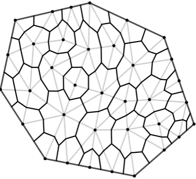
[image:7.595.204.406.102.287.2]● ●
Fig. 1. The dual mesh (black) is constructed by joining the centroids of the primal triangular mesh (grey). The vol-umes of these dual cells define the weights of an
integra-tion scheme based at the nodes of the primal mesh.
(2011) also show that these models lead exactly to the classical conditional autoregressive models when computed over a regular lattice. This model can be extended to non-stationary, anisotropic, multivariate and spatiotemporal random fields (Cameletti et al., 2013; Fuglstad et al., 2015), and the methods described in this paper extend to these cases in a straightforward way, although the
implementation of these models may be non-trivial. 245
The matrixB in (6) encodes information on the process on the boundary of the observation windowΩ. The effect of physical boundaries in spatial models has received very little attention in the literature. A notable example in the context of Bayesian smoothing is Wood et al. (2008). For the remainder of this paper, we will setB = 0, which corresponds to Neumann, or no-flux, boundary conditions. These specify that the normal derivative of the field at the boundary is zero 250
and can be physically related to an insulating boundary from which no heat escapes. We discuss the interpretation of this condition in Section 7·4.
We suggest a meshing strategy that constructs a regular triangulation of the observation win-dow, and refine it in areas where there are a large number of points. Point pattern data hold information on the relevant point process even in areas with only a few points. Hence, in order to 255
avoid approximation bias introduced by the choice of mesh, the triangulation needs to cover the space in a fairly regular way. On the other hand, we are unlikely to be able to infer the fine-scale latent structure in areas where we have no points or there has been little sampling. A detailed discussion of mesh selection can be found in Chapter 6 of Blangiardo & Cameletti (2015).
In order to complete the model specification, we must define an integration scheme to be used 260
in (3). The simplest option is to attach to each node in the mesh a regionVifor which the value
of the basis functionφi(s)is greater than the value of any other basis function. This
construc-tion, shown in Fig. 1, corresponds to the important notion of the dual mesh. The corresponding integration rule sets˜si to be the node location and α˜i =|Vi|to be the volume of the dual cell.
This approximation, known as the midpoint rule, is second-order accurate on a regular grid but 265
sum of optimal Gaussian integration rules on the individual triangles in the mesh. The weights and integration points for general triangles can be found in books on numerical analysis or finite element methods (Ern & Guermond, 2004). We discuss this further in the Appendix.
270
6. CONVERGENCE OF THE APPROXIMATIONS
The proposed method (3) for approximating the likelihood in a log-Gaussian Cox process has two distinct approximations: one to the integral in the likelihood and another to the latent Gaussian random field. Here, we show that both of these converge. The proofs and more general statements of all of the results can be found in the Appendix.
275
The first aspect of the approximation, discussed in Section 4, replaces the intractable inte-gral of the random intensity with a numerical quadrature scheme. The following theorem shows that, for any Gaussian random field Z(·), this approximation converges and the Hellinger dis-tance between the true posterior distribution and the posterior distribution constructed from the approximate likelihood is bounded by the error in the integration scheme.
280
THEOREM1. Assume thatZ(·)has, almost surely,ksquare-integrable derivatives, and that the p-point integration scheme in(3) has deterministic error of orderp−k. Then the Hellinger distance between the posterior distributions generated with the true and approximate likelihoods isO(p−k).
An interesting aspect of using stochastic partial differential equation models as our
finite-285
dimensional Gaussian random field is that the prior distribution converges as the mesh is refined (Lindgren et al., 2011; Simpson et al., 2012b). This is distinct from predictive processes or fixed-rank kriging approaches, where the finite-dimensional model (2) is taken as the true underlying model. The convergence of this approximation was established by Lindgren et al. (2011). The following theorem refines this result and shows that the approximate posterior distribution
con-290
verges weakly.
THEOREM2. Assume that the observation window is a convex polygon in R2 and let h be the maximum edge length in the mesh. Let Z(·) be the solution of (5)with α= 2. If G(·) is a uniformly Lipschitz continuous function, then the error in the posterior expectationE{G(Z)|y}
due to the stochastic partial differential equation approximation is of orderh1−for any >0.
295
7. EXAMPLES
7·1. Log-Gaussian Cox processes with extensions
We consider the application of log-Gaussian Cox processes in three increasingly complicated situations. In the first, a log-Gaussian Cox process with covariates is fitted to a real data set observed everywhere in a rectangular area (Rue et al., 2009; Illian et al., 2012). The second
300
example is a simulation study in the vein of Chakraborty et al. (2011), where the point pattern is incompletely observed due to varying sampling effort across the region of interest. The third case-study is inspired by the problem of mapping the risk associated with freak waves on oceans. We have constructed a point process defined only on the world’s oceans, i.e., over a very irregular, multiply-connected bounded region on a sphere. To the best of our knowledge, no other method
305
can be practically extended to fit a log-Gaussian Cox process in this situation.
● ● ● ● ● ● ● ● ● ● ● ● ●● ●●● ● ● ● ● ● ● ● ● ● ● ● ● ● ● ● ● ● ● ● ●● ● ● ● ● ● ● ● ● ● ● ●● ● ● ●● ● ● ● ● ● ● ● ●● ● ● ● ● ● ● ● ● ● ● ● ● ● ● ● ● ● ● ● ● ● ● ● ● ● ● ● ● ● ● ● ● ● ● ● ● ● ● ● ● ● ● ● ● ● ● ● ● ● ● ● ● ● ● ● ● ● ● ● ● ● ● ● ● ● ● ● ● ● ● ● ● ● ● ● ● ● ● ● ● ●● ● ● ● ● ● ● ● ● ● ● ● ● ● ● ● ● ● ● ● ● ● ● ● ● ● ● ● ● ● ● ● ● ● ● ● ● ● ● ● ●● ●●● ●●●●●●●●● ●● ● ●●●●●● ● ● ●● ● ● ●● ● ●●●●● ● ●● ● ● ●● ● ● ● ● ● ●●● ●●●●●● ● ● ● ● ● ●●● ● ●● ● ● ● ●●●●●● ●●●●●●●●●●● ● ● ● ● ●●●●● ● ● ●●●● ●●● ● ● ● ● ● ●●●●●●●●●●●●● ● ● ● ●● ● ● ● ● ● ● ● ● ● ● ●● ● ● ● ● ● ● ●● ● ●● ● ●●● ● ● ● ● ● ● ● ●●●● ● ●●●●● ● ● ● ● ●●● ● ● ●● ● ●●●●● ● ● ● ● ● ● ● ●●● ● ● ● ●●● ● ● ●●●● ● ● ● ● ● ● ● ●● ● ● ● ● ●●● ● ●●● ● ● ● ● ●●● ●●●●●●●●●● ● ● ● ●● ●●● ● ●● ● ●●●●●●●● ●● ●● ● ● ● ● ●●●●●●●● ● ●●● ●●●●●●● ●●●●●● ● ● ●●●●●●●●●● ● ● ● ●●●● ● ● ● ● ● ● ●●●●●●● ● ● ● ●●● ●● ● ● ●●●●●●●● ● ●● ● ●● ● ●●●●●●●● ● ●● ● ● ● ● ●●●●●●● ● ● ● ● ● ● ●●●●● ●●● ● ● ● ● ● ● ●●● ● ●●●● ● ● ● ● ●●●● ● ● ● ● ●●●●● ● ● ● ● ● ● ● ● ● ● ● ● ●●●●●●●●● ● ● ● ● ● ● ●●●●●●● ●● ● ●●● ● ●● ● ● ●● ●●● ● ● ● ● ● ●● ●●●●●●●● ● ● ●●● ●●●●●●●●● ●●●●● ● ●●● ● ●●●●●●● ● ● ●● ●●● ● ●●●● ● ●●●● ● ● ● ● ● ●● ● ● ● ●●● ● ● ●●● ● ● ● ● ● ● ● ● ●●● ● ● ● ● ● ● ● ● ● ● ● ● ● ● ● ●● ● ● ●● ● ●● ● ● ● ● ● ● ● ● ● ● ●● ● ● ●●●● ●● ● ●●●● ● ●● ● ● ● ●●● ● ●●●●●●●●●●●●● ● ●● ● ● ● ● ●●●●●●●●●●●●● ● ● ●● ●●●●●●● ●● ● ● ●●● ● ● ● ● ●● ● ●●●● ●●● ● ● ●●●●● ● ● ● ●●● ● ● ● ● ● ● ● ● ●● ● ●● ● ●● ● ● ● ● ● ● ●● ● ● ●●● ● ●● ● ●●●●●●●●●●●●● ● ● ● ● ● ●●●●●●●●●●● ● ●●● ● ● ●● ● ● ●●●● ●●● ●●●●●● ● ● ● ● ● ● ● ● ● ● ●●●●●●●●●●●●●● ● ● ● ● ● ●●●●● ● ● ● ● ● ● ● ● ● ● ● ●●● ● ● ●●● ●●● ●● ●●●● ●● ● ● ● ● ● ●● ● ● ● ● ● ● ● ● ● ● ●●● ●●●● ● ●●●● ● ●●● ●● ● ● ●● ● ● ●● ● ● ● ●● ● ●●●● ● ● ● ●●●●●●● ● ●● ● ● ● ● ● ● ● ● ● ● ● ● ● ●● ●● ●●● ● ● ● ● ●● ● ●●● ● ● ● ● ●● ● ● ● ●●●●●●●●●●●●●●●●● ● ● ● ●● ● ● ● ● ● ● ●● ● ● ● ● ●● ● ● ● ●● ● ● ● ● ● ● ● ● ● ● ● ● ●● ●●●●● ● ● ● ● ●● ● ●● ●●● ● ● ● ● ● ● ● ● ● ● ●● ● ● ● ● ● ● ● ● ● ● ● ● ●●●● ● ● ● ●●● ● ● ● ● ●● ● ● ●● ● ● ● ●●● ● ●● ● ● ●● ● ● ● ● ● ● ●●●●●● ● ● ● ● ●● ● ● ●● ● ● ● ● ●● ● ●● ● ● ● ● ● ● ●● ● ●●● ●● ● ● ● ● ●● ● ● ●●● ●● ● ● ● ● ● ● ● ● ● ●● ● ● ● ● ● ● ● ● ● ● ● ●● ● ●● ● ●● ●● ●●●● ● ●●● ●●● ●●● ●●●● ●● ●● ● ●●● ● ●● ● ● ● ● ● ●● ● ● ● ● ● ● ● ● ● ●● ●●●● ● ●●● ● ● ● ●●● ●● ● ● ● ● ● ● ● ● ● ● ●● ● ● ● ● ● ● ●● ● ● ● ●●●● ●● ●● ●● ● ● ●● ● ● ●● ● ●● ● ● ●●●●● ●● ●● ● ● ●● ● ● ●● ● ●● ● ● ● ● ● ● ● ● ● ● ● ● ●●●●● ●●● ● ● ● ● ● ●● ●● ● ● ● ● ● ● ● ●●●● ● ● ●● ● ● ●● ●●●● ● ● ● ● ● ● ● ● ●●●● ● ● ● ● ● ● ● ● ●● ● ● ● ● ● ● ● ● ●●● ● ● ● ● ● ● ●●●●● ● ●● ● ●● ●●● ● ● ● ● ● ● ● ● ●● ● ● ● ● ● ● ● ● ● ●● ● ● ●● ● ● ● ● ● ● ●● ● ● ● ● ● ● ● ●●● ● ● ●●●●● ● ● ●●● ●●●●●●●● ● ●●● ●●●●●● ● ●●● ● ● ● ● ● ● ● ● ● ● ●●●●●●●● ● ●● ● ● ● ● ● ● ●●●●●●●●●●●●●●●●●●●●●●●●● ● ● ●● ● ●●●● ●●● ●●●●●●●●● ●●●● ● ●●●●● ●●●●●●●●●● ● ● ● ● ● ● ●●●●●● ● ●●●●●● ● ● ●● ●●● ● ● ● ●● ● ● ● ● ● ●● ● ● ● ● ●● ●● ● ●● ● ● ● ● ● ● ●● ● ● ●●● ● ● ● ● ● ● ● ● ● ● ● ●●●● ●● ● ● ● ● ● ●● ●● ● ● ● ● ● ● ● ● ● ● ●●● ● ● ● ● ● ●●● ● ● ● ●●● ● ● ● ● ● ● ● ● ● ● ●● ● ● ● ● ● ●●●● ● ● ● ● ● ● ● ●● ● ● ●● ● ● ●● ● ● ● ●● ● ●●●●●●● ● ● ● ●●● ● ● ● ● ● ● ●● ●● ● ● ● ●●● ● ● ● ●● ● ● ● ● ● ● ● ● ● ● ● ●● ● ● ● ● ● ● ● ●● ● ● ● ● ● ●● ● ● ●● ●● ● ● ● ● ● ● ● ● ● ●● ●● ● ● ● ●● ●●● ● ● ● ● ●● ● ● ●● ● ● ● ● ● ● ●●● ● ● ● ● ●● ● ● ● ● ● ● ● ● ● ● ● ● ● ● ● ● ● ● ● ● ● ●● ● ●● ● ● ● ● ●● ● ● ● ● ● ●● ● ● ● ● ● ● ●● ● ● ● ●● ● ●● ● ● ●●●● ● ● ●●●● ● ● ● ●● ● ● ●● ●●●● ● ● ● ● ● ● ● ● ● ●●●●● ● ● ● ● ● ●●● ● ● ● ●● ● ●●●● ● ●●●● ● ● ● ● ● ● ● ● ● ● ● ● ● ● ● ● ● ●● ●●● ● ● ●●●●● ● ● ● ● ● ● ● ● ● ● ●● ● ● ●● ● ● ●● ● ● ● ● ● ● ● ● ● ● ● ●●● ● ● ●● ● ● ● ● ● ● ● ● ● ● ● ●● ● ● ● ● ● ● ● ● ● ● ● ● ● ●● ●● ● ●● ● ● ● ● ●●● ● ● ● ● ● ● ● ● ● ●● ● ● ● ● ● ● ● ● ● ● ● ● ●●● ● ● ● ● ●● ● ● ● ● ● ●●● ● ● ● ●● ● ● ● ● ● ●●● ● ● ●● ● ● ● ● ● ● ● ● ● ●●● ●● ● ●●● ● ● ● ●● ●● ● ● ● ● ●● ● ● ● ● ● ● ● ● ●● ●● ●●●● ● ● ● ● ● ●●●● ● ● ● ●● ● ● ● ●●● ●● ● ● ● ●●● ● ● ● ● ●● ● ● ● ● ●●● ● ● ●● ● ● ● ●● ● ●●● ●●●●● ● ●●●● ● ● ●● ● ● ● ●● ● ● ● ●● ● ●● ● ● ● ● ● ● ●●●●● ● ● ● ● ●●● ● ● ● ●● ● ●●●●●● ● ● ● ● ● ● ●● ● ●● ●●●●●● ●●● ●●●●●● ● ● ● ● ● ● ● ● ● ●●●●●●●● ● ● ● ● ●● ● ●● ● ● ● ● ● ● ● ●●●● ●● ● ● ● ● ● ● ● ● ● ● ● ● ● ● ● ● ● ● ● ● ● ● ● ● ● ● ● ● ● ● ● ● ● ●●●●● ● ● ●● ●● ● ● ●● ● ●● ● ● ● ●● ● ● ● ● ● ● ● ● ● ● ● ● ● ● ● ● ● ● ● ●● ● ● ● ● ● ● ● ● ● ● ● ● ● ●● ● ● ● ● ● ● ● ● ● ● ● ● ●● ● ● ● ● ● ● ●● ● ● ● ● ● ● ● ● ● ● ● ● ● ● ● ● ● ● ● ● ● ● ● ● ● ● ● ● ● ● ● ● ● ● ● ● ● ● ● ● ● ● ● ●● ● ● ● ● ●● ● ● ● ● ● ● ● ● ● ● ● ●● ● ● ● ● ● ● ● ● ● ● ● ● ● ● ● ● ● ●●● ● ● ● ● ● ● ● ● ● ● ● ● ● ● ● ● ● ● ●● ● ●● ● ● ● ● ● ● ● ● ● ● ● ●● ●●● ● ● ● ● ● ● ● ● ● ● ● ● ● ● ● ● ● ● ● ● ● ● ● ● ● ● ● ● ● ● ● ● ●●●●●● ● ●● ● ● ● ● ● ● ● ● ● ●● ● ●● ●● ● ●● ● ● ● ● ● ● ● ●● ● ● ●●● ●●● ● ● ● ● ● ●● ● ● ●●● ● ● ● ● ● ● ● ●●●● ● ● ●● ●●●● ● ● ● ● ●●●●●●● ● ● ●●● ● ● ● ●●●●●● ● ● ● ● ● ● ● ● ● ● ● ● ●● ● ● ● ●● ● ●●● ● ● ● ●● ●● ● ● ● ● ● ●● ● ● ● ● ● ● ● ●● ●● ● ●● ● ● ●●●● ● ●● ● ●● ●● ● ● ● ● ●●●● ● ● ● ●● ● ● ● ● ● ● ● ● ● ●●●● ● ●●● ● ● ● ● ●● ● ● ● ● ● ● ● ● ● ● ● ● ● ●● ● ●● ●● ● ● ● ● ● ● ● ● ● ● ● ● ● ● ● ● ● ● ● ● ● ● ● ● ● ● ● ● ● ● ● ● ● ● ● ● ● ● ● ● ● ● ● ● ● ● ● ● ● ● ● ● ● ● ● ● ● ● ● ● ● ● ● ● ● ● ● ● ●● ● ●● ● ● ● ● ● ● ● ● ● ● ● ● ● ● ● ●●●●● ● ●●● ● ● ● ● ●● ●●●● ● ● ●● ● ● ● ● ● ● ● ● ● ● ● ●● ● ● ● ● ● ● ● ● ● ● ● ● ● ● ● ● ● ● ● ● ● ● ● ● ● ● ● ● ● ● ● ●●● ● ● ●●●● ●●●● ● ● ● ● ● ● ● ● ● ● ● ● ● ● ● ● ●● ● ● ● ● ● ● ● ● ● ● ● ● ● ● ● ● ● ●●● ● ● ● ● ● ● ● ● ● ● ● ● ● ● ● ● ● ● ●● ● ● ● ●● ● ● ● ● ●● ● ● ● ● ● ● ● ● ● ● ● ● ● ● ● ●●●●●●● ●● ● ● ● ●● ●● ● ● ● ●●●● ● ● ● ● ● ● ● ● ● ● ● ● ● ● ● ● ●● ● ● ● ● ● ●●●●●●●●●●●● ●● ● ● ● ● ● ● ● ● ● ● ● ● ● ● ● ● ● ● ●● ●●● ● ● ●● ● ● ●● ● ● ● ● ●● ● ● ● ● ●●●●●● ● ●● ● ● ●●● ●● ● ● ● ● ● ● ● ● ●● ●● ● ● ● ● ●●● ● ●● ●●● ● ● ● ● ●● ●● ● ● ●● ● ● ● ● ● ● ● ● ●● ● ●●● ● ●● ●● ● ●● ●● ● ● ● ●●● ● ● ●●●●● ●● ● ● ● ●● ● ● ● ● ● ● ●●● ● ● ● ● ● ● ● ● ●●● ● ● ● ● ● ● ●● ●● ● ● ● ●● ●● ● ● ●● ● ● ● ● ● ● ● ● ●●● ● ● ● ● ● ● ● ● ● ● ● ● ● ● ●● ● ● ● ● ●● ● ● ● ● ●● ● ●● ● ● ● ● ● ● ● ● ● ● ●● ● ● ● ● ● ● ● ● ● ●● ● ● ● ●● ● ● ● ● ● ● ● ● ● ● ● ●● ● ● ● ● ● ● ● ● ● ●● ● ● ● ● ● ● ● ● ● ● ● ● ● ● ● ● ● ● ● ● ● ● ● ● ● ● ● ● ●● ● ● ● ● ● ● ● ● ● ● ● ● ● ● ●● ● ● ● ● ● ● ● ● ● ● ● ●●●● ● ● ● ● ● ● ● ● ● ● ● ●● ● ● ● ● ● ● ●● ● ● ● ● ●● ● ●● ● ● ● ● ● ● ● ● ● ● ● ● ● ● ● ● ● ● ●●●● ● ●● ● ● ● ● ● ● ● ● ●● ● ● ● ● ● ●● ● ● ● ● ● ● ● ● ● ● ● ● ● ● ● ● ● ● ● ● ● ● ● ●● ● ● ● ● ● ● ● ● ● ● ● ● ● ● ● ● ● ● ● ● ● ● ● ● ● ● ● ● ● ● ● ● ● ● ● ● ● ● ● ● ● ● ● ● ● ● ● ● ● ● ● ● ● ● ● ● ● ●● ● ● ●● ● ● ●● ● ● ● ● ● ● ● ● ● ● ● ● ● ● ● ● ●● ● ● ● ● ● ● ● ● ● ● ● ● ● ● ● ● ● ● ● ● ● ● ● ● ●● ● ● ● ●● ● ● ● ● ● ● ● ●●●● ● ● ● ● ●● ● ● ● ● ● ●● ● ● ● ●● ● ● ● ● ● ● ● ● ● ● ●●●● ● ●● ● ● ● ● ● ● ● ● ● ● ● ● ●● ● ●● ●● ● ● ● ● ● ● ● ● ● ● ● ● ● ● ●● ● ● ● ● ● ● ● ● ● ● ● ● ●● ● ● ● ● ● ● ● ● ● ● ● ● ● ● ● ● ● ● ● ● ● ● ● ● ● ● ● ● ● ● ● ● ● ● ● ● ● ● ● ● ● ● ● ● ● ● ● ● ● ● ● ● ● ● ● ● ● ● ●● ● ● ●● ● ● ● ● ● ● ● ●● ● ● ● ● ● ● ● ● ● ● ● ● ● ●● ● ● ● ● ●● ● ● ● ● ● ● ● ● ● ● ● ● ● ● ● ● ● ● ● ● ● ● ● ● ● ● ● ● ● ● ● ● ● ● ● ● ● ● ●●● ● ●● ● ● ● ●● ● ● ● ● ● ●● ● ● ● ●● ● ● ● ● ● ● ● ● ● ● ● ● ●●● ● ● ●●● ●●●● ● ● ● ● ● ● ● ● ● ● ● ● ● ● ● ● ● ● ● ● ● ●● ●● ● ● ●●●● ●●● ● ● ● ● ● ● ● ●● ●● ● ●● ●● ● ● ●●● ● ● ● ● ● ● ● ● ● ● ● ● ●● ● ● ● ● ● ● ● ● ● ● ●● ● ●●● ●● ● ● ● ● ● ● ● ● ● ● ● ● ● ● ● ● ● ● ● ● ● ● ● ●●● ● ● ●●● ● ● ● ● ●●●
0 200 400 600 800 1000
0 200 400 Easting Nor thing (a)
−0.1 0.0 0.1 0.2
0
4
8
Phosphorus
(b) Fig. 2. The effect of soil potassium levels on the loca-tion ofProtium tenuifolium. (a) The location ofProtium tenuifolium; (b) The posterior covariate effect of phospho-rus, using the standard lattice method (dashed), and the stochastic partial differential equation approach (solid).
Wherever not specified otherwise, we use independent Gaussian prior distributions with mean0 310
and variance100onlogκandlogτ. In all examples,α= 2.
7·2. Comparison with a lattice-based approach for rainforest data
This case-study is a standard application of spatial point processes, associating species with soil properties in tropical rainforests. The complete data set consists of the location of all trees with diameter at breast height of 1cm or greater, for a total of319tree species within a 50 ha 315
rainforest plot on Barro Colorado Island in Panama that has never been logged. We model the large spatial pattern formed by 4294 trees of speciesProtium tenuifolium, shown in Fig. 2(a), relative to the covariate phosphorus, which is given on an interpolated grid (John et al., 2007; Hubbell et al., 1999; Condit, 1998). The plot on Barro Colorado Island is only one plot within a large network of 50 ha plots t established as part of an international effort to understand species 320
survival and coexistence in species-rich ecosystems (Burslem et al., 2001).
Data sets with a similar structure have been analysed both with descriptive (Law et al., 2009) and model-based approaches (Waagepetersen, 2007; Waagepetersen & Guan, 2009; Wiegand et al., 2007). Integrated nested Laplace approximation can be used to fit a log-Gaussian Cox process to similar data, and also to a joint model of the pattern and covariates (Rue et al., 2009; 325
Illian et al., 2012). For illustration, we fit a simple model, where the latent field isZ(s) =µ+
βP(s) +x(s), whereµis a constant mean,P(s)is a spatially varying covariate describing the level of phosphorus in the soil andx(s)is an approximately intrinsic stochastic partial differential equation model with κ= 0.0014, which corresponds to a range much larger than the spatial domain. The parameter log(τ) is assigned a vague Gaussian prior distribution with mean zero 330
and variance1000.
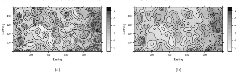
For comparison, we fit a lattice model with linear predictorz=µ1 +βP +x,where1is a vector of ones,Pthe phosphorus concentration,x∼N(0, τ−1Q−1)is an intrinsic second-order conditional autoregression (Rue & Held, 2005) and τ ∼Ga(1,10−5). Both models required around 25 seconds to fit in R-INLA. The posterior means for the spatial random effects are 335
Easting
Nor
thing
100 200 300 400
200 400 600 800
−7 −6 −5 −4 −3 −2
(a)
Easting
Nor
thing
100 200 300 400
200 400 600 800
−7 −6 −5 −4 −3 −2
[image:10.595.80.468.85.208.2](b) Fig. 3. Estimated spatial effects forProtium tenuifolium: (a) Using a standard lattice point process model; (b) Using
the stochastic partial differential equation approach.
7·3. Incorporating variable sampling effort
340
A major challenge when applying spatial point process models to real data sets is that the point pattern is rarely captured exactly, so sampling effort must be included in the observation process (Chakraborty & Gelfand, 2010; Chakraborty et al., 2011; Niemi & Fernandez, 2009). In this example, we consider the case where there is a sub-area in the data set with no measurements, but where presences are possible. This type of situation occurs, for instance, when considering
345
the spatial distribution of an animal species over an area that contains a region that is impossible to survey (Elith et al., 2006). In a related situation, data sampling effort varies spatially and is higher in areas where the scientists expect a good chance of presence, as in preferential sampling models (Diggle et al., 2010).
Following Chakraborty et al. (2011), we include known sampling effort in our model by
writ-350
ing the intensity asλ(s) =S(s) exp{Z(s)}, whereS(s)is a known function describing the sam-pling effort at locations. In this example, we assume that the point pattern has been observed perfectly, except in a rectangle where the pattern is not observed; see Fig. 4(a). We therefore defineS(s)to be zero inside this rectangle and unity everywhere else. It is straightforward to see from (1) that, with this choice ofS(s), the unsampled area does not contribute to the integral in
355
the likelihood. We can therefore choose the mesh to be quite coarse in this area, as long as this does not adversely affect the stochastic partial differential equation approximation to the random field. Figure 4(b) shows a mesh that has been coarsened in a rectangular region corresponding to a hole in the sampling effort. When coarsening the mesh, it is important to remember that we still want small triangles in the vicinity of the observed region, and we want these to gradually
360
change to larger triangles. This ensures that the stochastic partial differential equation approxi-mation is stable. In Fig. 4(b) this transition can be clearly seen. The changes to theR-INLAcode necessary to add sampling effort to basic point process code are minimal. This method can be extended in a straightforward manner to cover more complicated designs, although Chakraborty et al. (2011) suggest it is necessary to assume that the design is known.
365
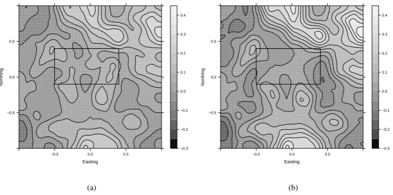
In order to test our method on this type of problem, we simulated a log-Gaussian Cox pro-cess on[−1,1]×[−1,1]and removed the points from the rectangle[−0.5,0.4]×[−0.1,0.4]to simulate the variable sampling. The simulated data set is shown in Fig. 4, and the difference in the posterior mean generated from the full data and the censored data is shown in Fig. 5. There is very little difference between the two posterior means outside the censored area, whereas
370
● ● ● ● ● ● ● ● ● ● ● ● ● ● ● ● ● ● ● ● ● ● ● ● ● ● ● ● ● ● ● ● ● ● ● ● ● ● ● ● ● ● ● ● ● ● ● ● ● ● ● ● ● ● ● ● ● ● ● ● ● ● ● ● ● ● ● ● ● ● ● ● ● ● ● ● ● ● ● ● ● ● ● ● ● ● ● ● ● ● ● ● ● ● ● ● ● ● ● ● ● ● ● ● ● ● ● ● ● ● ● ● ● ● ● ● ● ● ● ● ● ● ● ● ● ● ● ● ● ● ● ● ● ● ● ● ● ● ● ● ● ● ● ● ● ● ● ● ● ● ● ● ● ● ● ● ● ● ● ● ● ● ● ● ● ● ● ● ● ● ● ● ● ● ● ● ● ● ● ● ● ● ● ● ● ● ● ● ● ● ● ● ● ● ● ● ● ● ● ● ● ● ● ● ● ● ● ● ● ● ● ● ● ● ● ● ● ● ● ● ● ● ● ● ● ● ● ● ● ● ● ● ● ● ● ● ● ● ● ● ● ● ● ● ● ● ● ● ● ● ● ● ● ● ● ● ● ● ● ● ● ● ● ● ● ● ● ● ● ● ● ● ● ● ● ● ● ● ● ● ● ● ● ● ● ● ● ● ● ● ● ● ● ● ● ● ● ● ● ● ● ● ● ●● ● ● ● ● ● ● ● ● ● ● ● ● ● ● ● ● ● ● ● ● ● ● ● ● ● ● ● ● ● ● ● ● ● ● ● ● ● ● ● ● ● ● ● ● ● ● ● ● ● ● ● ● ● ● ● ● ● ● ● ● ● ● ● ● ● ● ● ● ● ● ● ● ● ● ● ● ● ● ● ● ● ● ● ● ● ● ● ● ● ● ● ● ●
−1.0 −0.5 0.0 0.5 1.0
[image:11.595.109.276.112.288.2]−1.0 −0.5 0.0 0.5 1.0 (a) (b) Fig. 4. Simulated data with a hole in the sampling effort. (a) The inner rectangle borders the area in which there was no sampling, and the plusses show the points that were missed due to incomplete sampling; (b) A mesh that takes into ac-count the lack of sampling effort in the rectangular region.
coarsened in the censored area, shown in Fig. 4(b). The posterior marginal distributions for the parameters for these two meshes are extremely similar. In order to avoid boundary effects in the 375
finite-dimensional random field, it is important to have points inside the censored area to ensure that the random field behaves properly. Use of the mesh correctly adapted to the problem resulted in a significant decrease in computational time. With the regular grid, the full inference took37
seconds on a Linux laptop with a 2.2 GHz i7 4702HQ processor, whereas the computation on the irregular mesh required only24seconds, a35%reduction by coarsening11%of the total mesh. 380
7·4. A point process over the ocean
In applications, point processes often occur over complicated domains rather than rectangles, and the topology, topography and geometry of the domain will typically be meaningful when modelling the covariance structure, see the discussion of Wood et al. (2008) in the context of spatial smoothers. For this case-study, we have simulated a log-Gaussian Cox process on the 385
oceans, motivated by a model for assessing the risk of freak waves.
The oceans form a non-convex, multiply-connected bounded region on the sphere and it is, therefore, necessary to construct a Gaussian random field model over this region. The main complication beyond those considered by Lindgren et al. (2011) is that we need a model for the covariance at the boundary. This difficult issue has been discussed very little in the statistics 390
literature. As we are working with simulated data, we can choose a relatively simple, yet realistic, boundary model. We expect that wave heights vary more near the coast than in the deep ocean and, as the designation of a freak wave is relative to the expected wave height, the random field is defined using the Neumann boundary conditions, which approximately doubles the variance
near the boundaries of the domain (Lindgren et al., 2011, Theorem 1). 395
Easting
Nor
thing
−0.5 0.0 0.5
−0.5 0.0 0.5
−0.3 −0.2 −0.1 0.0 0.1 0.2 0.3 0.4
(a)
Easting
Nor
thing
−0.5 0.0 0.5
−0.5 0.0 0.5
−0.3 −0.2 −0.1 0.0 0.1 0.2 0.3 0.4
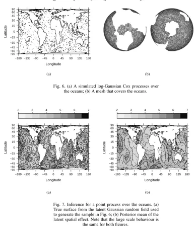
[image:12.595.84.467.113.303.2](b) Fig. 5. The posterior mean of the spatial effect for variable sampling effort (Section 7·3): (a) Using the complete sim-ulated point pattern; (b) Using the incomplete, partially ob-served point pattern. The large scale features of both fields are similar in areas in which the point pattern was sampled.
performed on this model and the posterior mean is shown in Fig. 7(b). The posterior mean shows the same large-scale features as the sample used to generate the log-Gaussian Cox process, see Fig. 7(a), with the expected loss of information due to the uninformative nature of point pattern
400
data.
Effects induced by the boundary conditions can be seen in Fig. 8. The pointwise posterior standard deviation of the latent Gaussian field is shown in Fig. 8(a). The standard deviation is reasonably constant away from the coasts, but is much higher near the boundaries. There are some interesting effects in the Gulf of Carpentaria in Australia, and in the North Sea. This is an
405
effect of the prior model, which increases the variance near the boundaries and in areas with high curvature of the coastline.
In the context of freak wave modelling, the most important result is displayed in Fig. 8(b), showing the probability that the log-risk will be greater than 5.5. Once again we see pro-nounced effects near the coastlines. This type of map can easily be computed using the function
410
inla.pmarginal in the R-INLA package. It is also possible to use the excursions package (Bolin & Lindgren, 2015) inRto construct joint exceedance maps.
8. DISCUSSION AND FUTURE WORK
The approximation to analyse log-Gaussian Cox processes introduced in this paper is valid also when using kernel methods (Higdon, 1998), predictive processes (Banerjee et al., 2008) or
415
fixed-rank kriging (Cressie & Johannesson, 2008). The problem with using these methods in the given context is that their basis functions are typically non-local and, therefore, the point evaluation matricesAiin (4) are dense; see Simpson et al. (2012b) for a further discussion of the
Longitude
Latitude
−90 −60 −45 −30 −15 0 15 30 45 60 90
−180 −135 −90 −45 0 45 90 135 180
(a) (b)
Fig. 6. (a) A simulated log-Gaussian Cox processes over the oceans; (b) A mesh that covers the oceans.
Longitude
Latitude
−90 −60 −45 −30 −15 0 15 30 45 60 90
−180 −135 −90 −45 0 45 90 135 180 2 3 4 5 6 7
(a)
Longitude
Latitude
−90 −60 −45 −30 −15 0 15 30 45 60 90
−180 −135 −90 −45 0 45 90 135 180 2 3 4 5 6 7
[image:13.595.94.484.86.536.2](b) Fig. 7. Inference for a point process over the oceans. (a) True surface from the latent Gaussian random field used to generate the sample in Fig. 6; (b) Posterior mean of the latent spatial effect. Note that the large scale behaviour is
the same for both figures.
In Section 7·4, we consider a point process over a complicated region of the sphere. To the 420
best of our knowledge, there are no other applicable inference methods for this example that include a covariance model at the boundaries. In general, modelling of boundary effects for point processes has not previously been discussed in the literature. We argue that by using Neumann, or no-flux, boundary conditions the variance at the boundaries increases. Similarly, Dirichlet boundary conditions, which correspond to fixing the value of the field at the boundaries, decrease 425
the variance. A future question is to construct good boundary models, and study their effect in a statistical context.
There is work to be done on the theoretical properties of the approximation presented in this paper. Some partial results are given in the Appendix, but they are not the complete story. In particular, it would be interesting to study the effect of both the likelihood approximation and the 430
Longitude
Latitude
−90 −60 −45 −30 −15 0 15 30 45 60 90
−180 −135 −90 −45 0 45 90 135 180 0.2 0.3 0.4 0.5 0.6 0.7 0.8 0.9 1.0 1.1
(a)
Longitude
Latitude
−90 −60 −45 −30 −15 0 15 30 45 60 90
−180 −135 −90 −45 0 45 90 135 180 0.0 0.2 0.4 0.6 0.8 1.0
[image:14.595.81.455.97.287.2](b) Fig. 8. Inference for a point process over the oceans. (a) The pointwise posterior standard deviation for the log risk surface; (b) The posterior risk mappr logλ(s)>5.5|y}.
control range, variance and, in more complicated cases, non-stationarity, are often of scientific interest and determining the rate of convergence will help us understand their interpretations.
Moving our considerations to more general finite-dimensional expansion (2), it is also of in-terest to quantify the link between the basis functionsφi(s)and the statistical properties of the
435
estimator. Although there has been work by Stein (2014), there are a number of open questions. This is a challenging problem as the interest is in non-asymptotic behaviour both in the number of basis functions and in the amount of data. In order to do practical spatial statistics, we need to give something up and often methods will be asymptotically incorrect. However, it may be that in realistic regimes, the resulting statistical error is manageable.
440
Finally, the approximation in Section 4 applies even when the latent random field Z(s) is not Gaussian. The only requirement is that it has the basis function expansion (2) and that the statistical properties ofzare known. In particular, this approximation applies to stochastic partial differential equation models with non-Gaussian noise. This has been investigated for type-G
L´evy processes, and especially for Laplace random fields (Bolin, 2014). Similarly, replacing
445
Gaussian white noise with Poisson noise would result in shot-noise Cox process models of the Mat´ern type. It may be possible to avoid the assumptions that the random field is Gaussian in the Appendix. The main use of Gaussianity is in the form of Fernique’s theorem, which is a statement about the tails of a Gaussian random field and it is possible that similar results would hold for non-Gaussian fields after modifying the growth conditions on the likelihood and the
450
functionals.
ACKNOWLEDGEMENT
The authors wish to thank the associate editor and the anonymous reviewers for their useful suggestions and, in particular, for pushing us to work out the convergence results. The authors gratefully acknowledge the financial support of Research Councils UK for Illian. We would also
455
The BCI forest dynamics research project was made possible by National Science Founda-tion grants to Stephen P. Hubbell: DEB-0640386, DEB-0425651,DEB-0346488, DEB-0129874, DEB-00753102, DEB-9909347, DEB-9615226, DEB-9615226, DEB-9405933, DEB-9221033, DEB-9100058, DEB-8906869, DEB-8605042,DEB-8206992, DEB-7922197, support from the 460
Center for Tropical Forest Science, the Smithsonian Tropical Research Institute, the John D. and Catherine T. MacArthur Foundation, the Mellon Foundation, the Small World Institute Fund, and numerous private individuals, and through the hard work of over 100 people from 10 countries over the past two decades. The plot project is part of the Center for Tropical Forest Science, a
global network of large-scale demographic tree plots. 465
APPENDIX
A·1. Likelihood approximation
Throughout this appendix, we assume that the parameters in the covariance model forZ(s)are known and fixed. We show that, for a fixed random fieldZ(s), the posterior distribution computed using the likelihood approximation converges strongly to the true posterior distribution, and the rate of convergence 470
can increase as the smoothness of the field increases. We also show that for either the true or approximate likelihood, the posterior distribution generated using the finite-dimensional stochastic partial differential equation model converges weakly to that generated using the limiting Mat´ern model. Finally, we show that under further assumptions the convergence rate depends both on the basis functions and the smoothness of the underlying random field. The main tools used in this appendix come from the inverse problems lit- 475
erature, surveyed in Stuart (2010), which deals with inference of indirectly observed continuous Gaussian random fields.
In order to show that the approximate posterior distributions converge to the true posterior distribution, it is useful to re-write the problem in terms of measures. Letµ0(A) =pr{Z(·)∈A} be the Gaussian
measure defined by the Gaussian random field prior measure onZ(·). If we define
Φ(Z;Y) =
Z
Ω
exp{Z(s)}ds− X
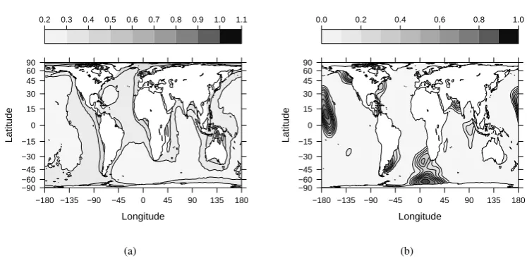
si∈Y
Z(si),
then the posterior probability measureµforZ(·)conditioned onY can be defined through its Radon– Nikodym derivativedµ/dµ
0(Z)∝M−1exp{−Φ(Z;Y)},whereM is a normalising constant required to
ensure thatµ is a probability measure. We can, in a similar fashion, define the approximate posterior 480
measure as
dµp
dµ0
(Z)∝Mp−1exp{−Φp(Z;Y)}, (A1)
whereΦp(Z;Y) =Pp
i=1α˜iexp{Z(˜si)} −Psi∈Y Z(si),andMpis a normalising constant. Cotter et al. (2010) showed that, under conditionsΦandΦp, the Hellinger distance
dHell(µ, µp) =
1 2
Z (dµ
dµ0 1/2
−
dµp
dµ0 1/2)2
dµ0
1/2
between the approximate and true posterior distributions converges to zero. Stuart (2010) notes that con-vergence in Hellinger distance implies concon-vergence in the total variation metric and it can be related to convergence of functionals using the identity
|Eµ{f(Z)} −Eµ0{f(Z0)}| ≤2Eµ{|f(Z)|2} −Eµ0{|f(Z0)|2}dHell(µ, µ0). (A2)
The following theorem shows that their theory applies to our approximate likelihood. 485
THEOREM A3. Consider a Gaussian random fieldZ(·)defined on a Lipschitz domainΩand assume
rule satisfies
Z
Ω
f(s)ds−
p
X
i=1
˜
αif(˜si)
≤Cψ(p)kfkHγ, (A3)
where ψ(p)→0 as p→ ∞ and γ≤α. Then, asp→ ∞, dHell(µ, µp)→0. Furthermore, if γ is an
integer, thendHell(µ, µp)≤Cψ(p).
490
Proof. This result follows directly from Theorem 2.4 of Cotter et al. (2010) if we can show that the
potential is bounded above and below and that the error in the likelihood approximation is integrable. LetkZ(·)k∞= sups∈Ω|Z(s)|, and letkYk be the number of points in the point patternY. Firstly we
note that, by assumption, kZ(·)k∞ andkYk are almost surely finite. Then, ifmax(kZk∞,kYk)< r, straightforward calculation shows thatΦ(Z;Y)≤ |Ω|er+r2.Similarly, whenkYk< r,
495
Φ(Z;Y) =
Z
Ω
exp{Z(s)}ds− X
si∈Y
Z(si)≥ −rkZk∞≥ −CrkZkHγ,
where the last inequality follows from Sobolev’s embedding theorem and is true for everyγ > d/2. Sim-ilar arguments show thatΦp(Z;Y)is also bounded above and below independently ofp.
To show that the error in the likelihood induces a similar error in the posterior distribution, we need to verify that, for sufficiently small >0, there exists a K >0 that does not depend on Z
500
such that|Φ(Z;Y)−Φp(Z;Y)| ≤Kexp kZk2
∞
ψ(p).By assumption, this reduces to showing that
kexp{Z(·)}kHγ≤Kexp(kZk2∞)for large enoughZ. Letγbe an integer. Now, for any realisation of
Z(·) :D→R, there exists an extensionIZ(·) :Rd→
Rsuch thatIZ(·)∈Hγ(Rd)has compact support and IZ|D(·) =Z(·). Using the quotient space structure of a Sobolev space on a domain, it follows that
kexp{Z(·)}kHγ(Ω)= inf
Hγ(Rd)3Z˜(s)=Z(s), a.s. s∈Dkexp{
˜
Z(·)}kHγ(Rd)
505
≤Cexp(kIZ(·)kL∞(Rd))
kIZ(·)kHγ(Rd)+kIZ(·)kγ Hγ(Rd)
≤Cexp(CkZ(·)k∞)
kZ(·)kHγ(Ω)+kZ(·)kγHγ(Ω)
,
where the first inequality follows from Theorems 2 and 3 of Bourdaud & Sickel (2010), the second in-equality follows from the boundedness of the extension operator and the constantCchanges from line to line.
510
Remark A1. The condition that γ is an integer can probably be relaxed, but it is an open question
whetherkexp{Z(s)}kHγ(Rd)can be bounded for non-integerγin the same way as in the integer case. If this was true, it would suggest the use of integration rules of orderdαerather thanbαcand would slightly improve the convergence rate.
The techniques used to prove Theorem 3 also allow us to give a more informative convergence result
515
for the traditional counting process approximation to the log-Gaussian Cox process than those considered by Waagepetersen (2004).
COROLLARY A1. Assumeα≥2. Then the classical(p+ 1)×(p+ 1)lattice approximation to the
log-Gaussian Cox process converges in the Hellinger distance at a rate ofO(p−1).
Proof. For simplicity, we will assume that the observation windowDis square and the lattice is equally
520
spaced in both directions. The lattice approximation is of the form (A1) with
Φp(Z) = p
X
i,j=1
|Sij|exp{Z(˜sij)} − p
X
i,j=1
kY ∩SijkZ(˜sij), (A4)
whereSij is the(i, j)lattice cell and˜sij is the centroid ofSij. The first term in (A4) is the midpoint rule approximation to R
ψ(p) =p−γ (d/2< γ≤2), (Theorem 8.5, Ern & Guermond, 2004). The error in the likelihood arising from the approximation of Z(sk)byZ(˜sij)for anysk∈Y ∩Sij can be bounded using Taylor’s the- 525
orem as |Z(sk)−Z(˜sij)| ≤p−1sups∈Sijsup`=1,...,d
∂Z(s)
∂s`
≤Cp
−1kZk
H1+d/2(Sij), where the sec-ond inequality is a consequence of Sobolev’s embedding theorem (Brenner & Scott, 2007, Corol-lary 1.4.7). It follows using the arguments in the proof of Theorem 3 that for a two-dimensional lat-tice,|Φ(Z)−Φp(Z)| ≤CkYkp−1kZk
H2(Ω), and the result follows from Theorem 2.4 of Cotter et al.
(2010). 530
Remark A2. Examining the proof of Corollary A1, it can be seen that the rate of convergence is
de-termined by the binning procedure and using the lattice quadrature rule and the approximate likelihood proposed in this paper the rate of convergence would beO(p−2)for smooth enough fields.
A·2. Random field approximation
While Appendix A·1 shows that for fixedZ(·)the likelihood approximation introduced in this paper 535
converges, this is not enough to show that the posterior distributions computed in Section 7 converge as we are simultaneously approximating the log-Gaussian Cox process likelihood and the Gaussian random field using the approximation outlined in Section 5. In this appendix, we close this gap when the hyper-parameters are fixed and show the convergence of a general class of finite-dimensional approximations to problems in which the indirectly observed unknown random function is equippeda prioriwith a Gaussian 540
random field.
There are a number of technical challenges to showing convergence of this approximation. The first is that we need to compare a measure on an infinite-dimensional space with a sequence of measures on different finite-dimensional spaces. We will, therefore, no longer be able to consider convergence in the Hellinger metric, but rather we will consider a weaker mode of convergence of an approximating mea- 545
sureνn,ptoµ, that is the convergence of functionals of the formR
G(Zn)dνn,p(Zn)→
R
G(Z)dµ(Z),
for Lipschitz continuous functions that satisfy a growth condition to ensure the functionals are finite. This is slightly stronger than convergence in distribution, for which bounded Lipschitz functions suffice (Bogachev, 2007, Section 8.3). When the finite-dimensional approximation to the Gaussian random field is computed by truncating its Karhunen–Lo`eve expansion, Dashti & Stuart (2011) showed convergence. 550
Their techniques, which relied heavily on the idea that truncation of the Karhunen–Lo`eve expansion is an
L2(Ω)projection, are not directly applicable to the approximation outlined in Section 5.
In Section A·3, we extend Theorem 2.6 of Dashti & Stuart (2011) to a general class of finite-dimensional approximations. In particular we show that if the approximation Zn(·) toZ(·)is stable, in the sense thatkZnkH≤CkZkH uniformly inn, then the convergence of the functionals is governed 555
by the deterministic error in the pathwise approximation. In Section A·4 we show that for approximations of the general form of the stochastic partial differential equation approximation, this error is controlled by the ability of the finite-dimensional basis functions to approximate realisations of the true prior model. These results mirror previous quantitative results (Simpson et al., 2012a,b; Bolin & Lindgren, 2013), in which the stable, convergent approximation properties of piecewise linear functions were used to argue 560
for the adoption of stochastic partial differential equation models.
A·3. A general result on the convergence of finite-dimensional approximations
Let V ⊂H be Banach spaces and assume that k·kH ≤Ck·kV. Assume that the Gaussian random fieldZ(·)has paths almost surely inV and define the approximate random fieldZn(·) =RnZ(·), where
Rn:V →Vn is a deterministic linear operator, andVn⊂H is ann–dimensional vector space that is 565
not necessarily a subspace ofV. In the special case thatVn⊂V andRnis a projector, the arguments of Dashti & Stuart (2011) can be used to show convergence.
Extending the notation from Appendix A·1, we defineµ0(·)to be the law ofZ(·)and consider the
infinite-dimensional posterior distributionν(·)defined bydµ/dµ
0=M−1exp{−Φ(Z;Y)}.Similarly, we
define the law ofZn(·)to beν0n(·)and define the approximate posterior distributionsνn,pasdν
n,p
/dνn
0 = 570
M−1