Chaotic dynamics in flows and discrete maps

warwick.ac.uk/lib-publications

A Thesis Submitted for the Degree of PhD at the University of Warwick

Permanent WRAP URL:

http://wrap.warwick.ac.uk/98867

Copyright and reuse:

This thesis is made available online and is protected by original copyright.

Please scroll down to view the document itself.

Please refer to the repository record for this item for information to help you to cite it.

Our policy information is available from the repository home page.

CHAOTIC DYNAMICS IN

FLOWS AND DISCRETE MAPS

ANTHONY CURRIE

Department of Physics University of Warwick

This thesis is submitted to the

University of Warwick in partial fulfilment of the requirements for admission to the degree of Doctor of Philosophy

JANUARY 1987

SUMMARY

This work attempts to utilise perturbation theory to derive

discrete mappings which describe the dynamical behaviour of a

continuous, and a discrete, chaotic system.

The first three chapters Introduce some background to the

theory of chaotic behaviour In discrete and continuous systems.

Chapter 4 considers the dynamical behaviour of Duffings equation.

Perturbation theory is applied to Hamiltonian solutions of the

system, and a 1-D mapping is derived which models the bifurcation of

the system to chaos. Chapter 5 Introduces a 2—D chaotic difference

map. The qualitative dynamics of the system are Investigated and a

form of perturbation theory Is applied to a parameterlsed version of

the map. The perturbative solutions are shown to exhibit dynamical

behaviour very like the original system.

TABLE OF CONTENTS

SECTION TITLE

SUMMARY

TABLE OF CONTENTS

ILLUSTRATIONS ACKNOWLEDGEMENTS DECLARATION PAGE (i) (li.lii) (iv.v) (vi) (vil)

Chapter 1 INTRODUCTION 1

1.0 Background 1

1.1 Discussion 3

1.2 Overview of Thesis 4

CHAPTER 2 CHAOS IN FLOWS 6

1.0 Introduction 6

1.1 Regular Flows 6

1.2 Chaotic Flows 10

2.0 Routes to Chaos 11

2.1 Local Codimension 1 Bifurcations 11

2.2 Global Bifurcations 13

3.0 Characterisation of the Chaotic State 17

3.1 No Stable Periodic Orbits 17

3.2 Sensitivity to Initial Conditions 18

3.3 Mixing Behaviour 18

3.4 Ergodlclty 19

3.5 Lyapunov Exponents 19

3.6 Hyperbollclty 20

3.7 Strange Attractors 21

4.0 Examples of chaotic Systems 22

4.1 Hamiltonian Systems 22

4.2 The Lorens System 25

4.3 The Duffing System 27

CHAPTER 3 CHAOS IN DISCRETE MAPS 31

1.0 Introduction 31

1.1 Maps on an Interval of R 31

1.2 Bifurcations of Stable Periodic Orbits 33

1.3 Felgenbaum Sequences 34

1.4 Lyapunov Exponents 35

1.5 Probability Distributions 36

1.6 Summary 39

2.0 Examples of 2-D Discrete Systems 39

2.1 The Henon Map 39

2.2 The Chirikov Map 42

TABLE OF CONTENTS (CONTINUED)

SECTION TITLE PAGE

CHAPTER 4 DUFFINGS EQUATION 44

1.0 Background and Aim 44

2.0 Analytical Results 46

2.1 Multiple Scales Method 46

2.2 The Integral Method 57

2.2.1 The Outside Orbits 58

2.2.2 The Inside Orbits 73

3.0 Discussion 78

CHAPTER 5 THE SYMMETRIC MAP 80

1.0 Introduction 80

1.1 The Map 82

1.2 Strange Attractor 84

1.3 Investigation of the Symmetric Map 85

1.3.1 The Diagonal Map 85

1.3.2 Period 4 Attractor - Enslaving 85

1.3.3 Lypaunov Exponents and Boundary Behaviour 87

1.3.4 Conclusion 90

2.0 Parameterlsed Map 91

2.1 Analytical Results 94

2.2 Numerical Results 99

CHAPTER 6 CONCLUSION 103

APPENDIX A 106

APPENDIX B 108

APPENDIX C 115

REFERENCES 125

ILLUSTRATIONS

NUMBER HEADING FACING PAGE

NUMBER

2a Islands and Séparatrices of a Perturbed

Hamiltonian

22

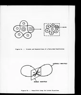
2b Homoclinic Loop for Lorenz Equations 22

2c Duffing Equation Phase Plane for f ■ 6 ■ 0 28

2d Poincaré Map for Duffing Attractor 28

3a Logistic Map for X ■ 2 33

3b Bifurcation Diagram for Logistic Map 33

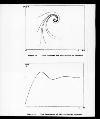
4a Phase Portrait for Multiple-Scales Solution 50

4b Time Dependence of Multiple-Scales Solution 50

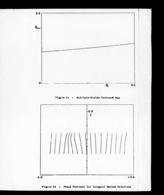
4c Multiple-Scales Poincaré Map 56

4d Phase Portrait for Integral Method Solutions 56

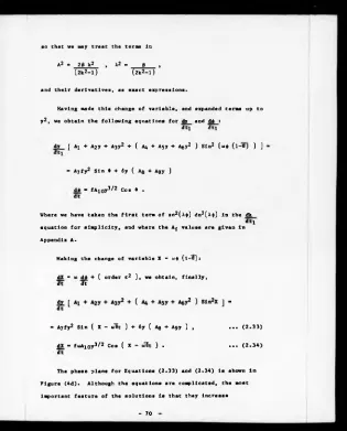
4e Poincaré Maps for Outside Orbits 73

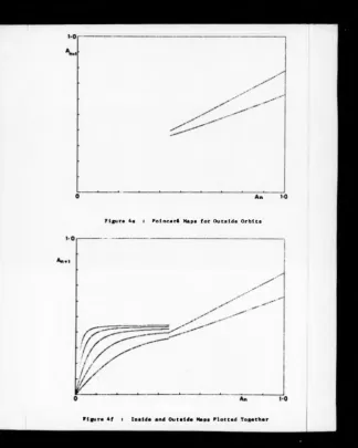
4f Inside and Outside Maps Plotted Together 73

«8 Suggested Form of Poincaré Map 77

Sa Symmetric Map Attractor 84

5b Cross-Plots of Bifurcation Diagrams 86

5c Iterates of J - 0 Line 86

Sd Attractor for a ■ 1.02 92

ILLUSTRATIONS Contd...

NUMBER

5e

5f

5g

Sh

HEADING PACING PAGE

NUMBER

Attractors for Various Values of a 93

Perturbation Solutions for Various Values 100

of 6a

Amplitudes for 6a " 0*165 100

Amplitude Maps for Two Values of 6a 101

ACKNOWLEDGEMENTS

I would like to thank all staff and students of the Physics

Departaent at Warwick with whom I had many stimulating discussions

and happy tlaes. Special thanks are due to Dr. George Rowlands for

his help and guidance, and for the many Informal tutorials held at

various bars around Warwickshire. I also thank my wife Suzanne for

bearing with me during the writing of the thesis.

For financial support, I thank the Science and Engineering

Research Council for a three year studentship, and the Marconi

Research Centre for use of Its word processing staff and

facilities.

DECLARATION

Except where otherwise Indicated, this thesis contains an

account of my own Independent research undertaken In the Department

of Physics, University of Warwick, between October 1982 and

September 1985 under the supervision of Dr. G. Rowlands.

CHAPTER 1

INTRODUCTION

1.0 Background

During the last century, attempts to formulate solutions to the

three body problem of classical mechanics led to the development of

the Hamiltonian formulism of mechanics. Up until this time It was

naturally believed that the asymptotic behaviour of all mechanical

systems was reducible to combinations of 'simple' forms such as

oscillatory or stationary (equilibrium) behaviour. This situation

ceased with the realisation, by PolncarS, of the extremely

complicated motion present near the fixed points of a perturbed

Hamiltonian system.

Concurrent with Poincaris observations regarding perturbed

Hamiltonian systems, were the results due to Boltzman who

considered the behaviour of gases to be explicable In terms of the

random motion of very many molecules, each of which could explore

the whole of state-space energetically available to it. This

'Ergodlc hypothesis' formed the basis of classical statistical

mechanics.

Given the possibility of stochastic behaviour in perturbed

Hamiltonian systems and systems with many degrees of freedom, the

problem remained as to how stochastic behaviour could be reconciled

with physical observations. It was apparent, for example, that the

solar system had remained relatively stable over hundreds of

millions of years.

This remained an unsolved problem until the 1950's when

Kolmogorov, and later Arnold and Moser postulated the so-called KAM

-theorem. The theorem implies that, for systems perturbed sway from

Integrable ones, the motion remains regular for most Initial

conditions. Whilst stochastic regions exist In the phase plane,

they are bounded by Invariant surfaces (KAM surfaces) which restrict

the stochastic motion. The Ergodlc hypothesis, therefore, was

found not to hold In general.

The study of chaotic systems p.r se did not advance

significantly beyond Polncarés work until the 1960's, when E. Lorenz

published his seminal paper on chaotic motion In a dissipative

system [22].

Lorenz observed that the numerical solutions of a set of

coupled non-linear ordinary differential equations appeared to be

attracted to a subset of phase space In which the aolutlon curves

wandered In an erratic manner. Ruelle and Takens were later to

coin the term 'strange attractor' to describe such attracting sets

on which chaotic motion occurred.

Since Lorenz's work, many strange attractors have been found

to appear In numerical solutions of differential equations. As the

equations are usually derived from a physical system; In Lorenz's

case the equations are abstracted from fluid equations. It would

seem that the chaos found In numerical observations is related to

physical notions of stochastlcity such as turbulence in a fluid etc.

However, the link between mathematical and physical chaos has still

to be made precise.

A great simplifying procedure in the study of strange

attractors Is to consider the Poincaré map of the system. This

reduction of the chaotic motion to one or two dimensions leads

naturally to consideration of chaos In discrete mappings of a line

or plane. The nature of chaotic behaviour In one dimensional

non-lnvertlble discrete maps in now well understood, much pioneering

work being due in this regard to Collett and Eckmann |10J • The

development of high powered computers in the last two decades has

enabled the highly complex, fractal, structure of strange attractors

to be elucidated by Iteration of the governing differential or

difference equation many thousands of times.

Observation of the global behaviour of the system in this way

can suggest a reduction of the full system to a form amenable to the

methods of symbolic dynamics - the underlying mathematical basis of

abstract chaotic systems.

An Important mathematical development In the study of chaotic

systems has been the Introduction of bifurcation theory. This

subject considers the changes In phase space topology resulting from

variation of a parameter of the system, and provides an Insight

into the various routes a 'regular' system may take to a chaotic

state.

1.1 Discussion

The preceedlng section gave a very short account of

developments in the subject of chaotic dynamics since Polncart.

There are many Inherent difficulties in this subject, not least

of which Is the problem of actually defining the chaotic state.

In the following two chapters, the chaotic state will be

A second difficulty is that it is impossible to rigorously

prove the existence of chaos in a system, for all but a few (mostly

abstract) systems« In considering systems such as Dufflags'

equation or the HSnon map, all that may be said is that the aystem

appears to possess a strange attractor which persists for many

iterations of the equations.

A final problem is that of obtaining an overall picture of the

various routes to chaos. Bifurcation theory has provided a general

picture of various instabilities in parameterlsed systems, but the

subject is Inherently messy and Incomplete. In particular, an

elucidation of the link between local, and global, bifurcations and

their relationship to the appearance of strange attractors is needed

to provide a coherent overview of chaos in flows and discrete

maps.

1.2 Overview of Thesis

The thesis falls naturally into two parts. The first is

concerned with chaos in Duffing's equation, and the second with a

chaotic discrete two-dimensional map.

The aim of the work on Duffing's equation is to attempt to

analytically derive a Poincart map for the system using perturbation

theory. A new perturbation method is developed in order to deal

with the special symmetries of the Duffing system. The resulting

equations are found to be too complicated to solve in two

dimensions, however, a one-dimensional discrete map is derived from

consideration of the amplitude equation and is indicated as a good

candidate for deacribing the period doubling of the system to

chaos.

-The second part of the thesis considers the characteristics

of a coupled logistic map which is referred to here as the eymmetric

map. The chaotic nature of the system can be understood

qualitatively by consideration of the foldings near singularities

of the map. The Lyapunov exponents of the system are numerically

obtained and their relevance discussed.

Finally, a form of perturbation theory is applied to a

pararneterlsed form of the map. The results give the limit cycle

solution observed in the system, which subsequently bifurcates to

chaos. The correspondence between the chaos of the original map and

that of the perturbation solution is discussed.

Before describing these results, a general introduction to

chaotic behaviour in flows and discrete maps will be given in the

following two chapters.

The thesis ends with a short resumé of results and

CHAPTER 2

CHAOS IN FLOWS

1.0 Introduction

This chapter Introduces some of the background material

pertaining to chaotic dynamics In flows. In this section, the

asymptotic behaviour to be expected of a one or two dimensional

system Is briefly described, followed by an overview of chaotic

behaviour In three or more dimensional systems. Section 2 considers

various routes by which a deterministic system may become chaotic

upon variation of a parameter. This involves a brief description of

local bifurcations In parameterlsed systems and also a consideration

of global bifurcations including homocllnlc tangencles and

Intersections.

The third section attempts to give a characterisation of the

chaotic state. Some definitions are taken from the field of

dynamical systems, in order to fix Ideas, and the concept of a

'strange attractor' Is Introduced.

The final section gives three examples of systems which exhibit

chaotic behaviour. One system In particular - the Duffing system -

Is considered In some detail as this system will be subsequently

studied In Chapter 4.

1.1 Regular Flows

The flows In this chapter are determined by systems of ordinary

differential equations of the form:

*»■ f<*> •

•••(K1)

dt

-where x ■ x(t) e Rn li a vector function of tine, and f:U ♦ Rn la

a smooth vector field defined on D c R n . We then define the 'flow*

generated by f to be a smooth function +(t,x):U x R ♦ Rn ,

(defined V x c Rn and for t In some Interval (a,b)) which satisfies

Equation 1.1, l.e.

d_ (♦(t.x))t-to - «(♦(to.*)) • . . . (

1

2

dt

Of particular Interest la the 'asymptotic' behaviour of a given

flow l.e. the behaviour of +(t,x) V x e U as t ♦

In this respect, the points x e U such that f(x) “ 0, assume

particular Importance as solutions Initiated at these 'fixed points'

remain there for all time. Remembering that +(t,x) Is a smooth

function, the question Is then 'what are the consequences for the

flow of having fixed points In U?' this question Is answered by way

of 'stability analysis'.

The fixed point "x is said to be 'stable' If for every

neighbourhood V of "x 3 vl ••*. every solution +(t,xQ ) with x© eVi

lies In V Vt > 0.

If, In addition to the above, can be chosen such that

x© eVi ->

4

stable.'

If none of the above apply, then "x Is said to be 'unstable'.

For flows In two, or more, dimensions, solutions may be attracted to

(or repelled from) a closed orbit, In this case we have a limit

cycle In the flow. The stability of a given limit cycle Is defined

by obvious extension of the definition above except now the fixed

points x are replaced by periodic solutions x(t). We may view

-'area preserving' flows, such as Hamiltonian flows, as systems

possessing stable (but not asymptotically stable) limit cycles«

It is apparent, then, that local behaviour of a flow may be

obtained by studying the stability of fixed points of the system.

The stability of a given fixed point is determined by the

eigenvalues of the system linearised about the fixed point. Thus,

given an equilibrium point x of Equation 1.1, the linearised system

is given by:

i

He now define three invariant subspaces of the 'state-space', (l.e.

the space in which solutions to Equation 1.1 lie) as follows [15]:

Es - SPAN (Vl...V*»*), En - SPAN {U*... D®u ) ,

EC - SPAN {W1 ,..., Wnc) ... (1.4)

where the V 1 , are the n, eigenvectors whose eigenvalues have

negative real parts, the U* are the ly, eigenvectors whose

eigenvalues have positive real parts, and the H* are the

eigenvectors whose eigenvalues have zero real part.

E*, Eu , and E c are called the 'stable', 'unstable' and 'centre'

subspaces respectively, reflecting the fact that solutions in E s are

characterised by exponential decay, solutions In Eu by exponential

growth, and solutions in Ec by neither.

The linear eigenspaces E*, and E u for system 1.3 have analogues

for the (possibly) non-linear system 1.1. In this caae we define

W 8loc - {xeU | 4>(t,x) ♦ x as t ♦ “ , and 4(t,x) eU Vt > 0} ,

. . . ( 1 . 5 )

wuioc - {xeU | ♦(t.x) ♦ x as t ♦ -, and ♦(t.x) eU Vt < 0} ,

where U Is a neighbourhood of x.

The 'Stable Manifold Theorem' [15] then tells us that given a

fixed point x with associated elgenspaces E 8, Eu , then there exist

local stable and unstable manifolds for x, which are tangent to E 8 ,

E u , at the equilibrium point.

Global stable and unstable manifolds are defined by iteration

of the corresponding local ones, l.e.

»•(*> - U ft (V8loc0 0 )

t<0 *

wu ( x ) - U (W«l o c ( 7 ) ) . . . ( 1 . 6 )

t>0

Stable and unstable manifolds of a limit cycle can be defined In an

analogous manner.

We shall see in later sections that the behaviour of stable and

unstable manifolds of a system can give global Information on the

flow.

The above discussion has Introduced the concepts of fixed

points and limit cycles for an n-dlmensional flow. It turns out

that in less than 3 dimensions, the asymptotic behaviour of a flow

Is completely determined by such structures.

The so-called Poincar£-Bendlxon Theorem [2] states, In

effect, that If an attracting (or repelling) set exists for a 2

dimensional flow, then It Is either a fixed point or a limit cycle.

Similarly, for a one dimensional flow, only fixed points may exist.

Thus, we may completely classify the types of behaviour to be

expected from a linear system of dimension n, or a non-linear

system of dimension one or two.

1.2 Chaotic Flows

For the case of a non-linear system of dimension greater than

two, a qualitatively different type of asymptotic behaviour can

occur. Typically, solution curves wander around some subset of

state-space In a seemingly random manner, without collapsing Into a

fixed point or limit cycle. This type of behaviour has been

labelled 'chaotic'. Although there is no agreed definition of a

chaotic system, It is possible to state various attributes which

may or may not be present In such a system, Section 3 of this

chapter attempts such a characterisation.

The subspace around which trajectories wander Is generally

kncwn as a 'strange attractor', although these objects are

extremely complex It Is possible to reduce the complexity of the

system by taking a 'Polncar£ map' of the flow. This mapping Is

generally defined on a two-dimensional surface which lies transverse

to the flow. If the first point of intersection of the flow with

the 2-D plane Is labelled Xq, then the PolncarS map P : R2 ♦ R2 is

formally defined by xi - P(xD), where xi Is the second point of

Intersection, X

2

2

apparent that an analytical form for P(x) m ay not exist, although

Before considering the characteristics of chaotic systems, a

discussion of the various routes to chaos will be given in the

next section.

2.0 Routes to Chaos

A situation which commonly occurs is that a system of

differential equations whose solutions are 'well behaved' may be

perturbed to a set of equations whose solutions appear random, or

chaotic. Considering the system to be parameterlsed with some

parameter, p, l.e.

£ - Fp(£) , M e R ... (2.1)

then we may study the family of Equations 2.1 as p is varied in some

Interval containing the parameter pc, where:

£ " Ppc(£) our chaotic system. The nature (or topology) of the

flows of Equation 2.1 will change in a certain manner as p ♦ pc,

thus giving a qualitative link between well-behaved and chaotic

systems.

The above methodology is known as 'bifurcation theory'. In

this section a brief discussion of the various codimension 1

bifurcations Is given, followed by a consideration of global

bifurcations.

2.1 Local Codimension 1 Bifurcations

We restrict ourselves to local codimension 1 bifurcations l.e.

bifurcations which occur near fixed points of one-parameter systems.

Given a parameterlsad system:

-which has an equilibrium at some point (pD , pG), we “ay form the

linearised system:

i - U . C - (x-p) ... (2.2)

If the matrix L has no eigenvalues which are zero or pure Imaginary

then p Is called 'hyperbolic' . Such hyperbolic fixed points are

'structurally stable' In the sense that they remain hyperbolic

when the system Is perturbed In a suitable way [15].

For a fixed point without zero eigenvalues, the 'Implicit

Function' theorem Implies that there Is a smooth function g(p) of

equilibria passing through (p0,p0) l.e. there Is no change In the

number of equilibria at (p0 ,|i0). If, however, the point has a zero

eigenvalue, then several branches of equilibria may come together

and we have a 'bifurcation point'.

It can be shown that there are four generic codimension 1

bifurcations, epitomised by the following systems [18].

x ■ p - x2 (saddle-node)

x ■ px - x2 (transcrltlcal)

x ■ px - x3 (pitchfork)

x - -y ♦ x (p - (*2 «. y2)))

y - X + y (p - (x2 + y2 ))

j

The saddle-node bifurcation corresponds to the creation of a

stable and an unstable equilibrium, In this case there Is no

'unperturbed solution' from which the equilibria bifurcate, In a

sense they are created from nothing.

The transcrltlcal bifurcation occurs when a stable and an

unstable equilibrium exchange their stability, and the pitchfork

bifurcation corresponds to an equilibrium splitting Into

2 equilibria, this 'period doubling' bifurcation will be

encountered many times In the discussion of chaotic systems.

The two-dimensional Hopf bifurcation occurs when an equilibrium

possesses two pure Imaginary eigenvalues. In this case a fixed

point bifurcates Into a periodic orbit, again, the Hopf bifurcation

will be encountered often In the following chapters.

This completes the discussion of local codimension 1

bifurcations. The theory of bifurcations In 2 or more codimension

systems Is difficult and far from complete, further details may be

found In [18].

2.2 Global Bifurcations

In previous sections the concept of a hyperbolic fixed point

was Introduced. In this section, we will consider a common type of

global bifurcation which occurs for systems possessing a particular

kind of hyperbolic fixed point known as a 'saddle'. A fixed point

x c Rn for a system of the form (1.1) Is called a 'saddle point'

if the system linearised about x has at least one eigenvalue with

negative real part, and at least one eigenvalue with positive real

part. In this situation, x will have associated stable and unstable

manifolds passing through it.

- 13

Although, by the theory of existence and uniqueness of

solutions for a system like (1.1), a stable or unstable manifold may

not Intersect Itself In state-space, It Is quite possible for the

stable manifold of one point to be Identified with the unstable

manifold of another point, In this case we have a 'saddle

connection' between the two points. It Is also possible for the

stable manifold of a point to be Identified with the unstable

manifold of the same point, In which case we have a 'saddle-loop' or

'homocllnlc orbit'. Such structures are very common In Hamiltonian

systems such as the ordinary pendulum, or Duffing's equation with

zero forcing and damping [p(44)].

The saddle-loop as described above Is structurally unstable,

l.e. If a system possessing a saddle-loop Is perturbed, then the

saddle-loop will disappear, or rather, deform Into some new

structure. This Is an example of a 'global bifurcation'.

Three possibilities exist for the form of the new structure

created after the perturbation: (1) the saddle-loop breaks, the

unstable manifold lies outside the stable one, (11) as (1) with the

stable manifold lying outside the unstable one, (111) the

perturbation Is time dependent and the stable and unstable manifolds

Intersect an Infinite number of times when they are viewed on a

surface of section (Polncar£ map).

Although It Is difficult to say precisely what has happened to

the flow In case (111), It can be proved that the appearance of

'homocllnlc Intersections' for the Polncari map Implies the

existence of a 'Smale-horseshoe' [34]. The horseshoe Is the product

periodic orbits of all periods and an uncountable set of nonperiodic

motions. Therefore, If we observe the intersection of stable and

unstable manifolds in the PoincarS map of the system we know that

very complex orbits exist In the flow. However, the horseshoe does

not attract anything, therefore, we cannot say that the system is

automatically chaotic l.e. that a strange attractor exists, rather,

the above bifurcation Is Important as It often preceeds global

chaotic behaviour of a system (c.f. Duffing's system Section 4.3)

The existence of a horseshoe In the Polncar£ map of a flow can lead

to a phenomenon known as 'preturbulence' [33] in which orbits

wander erratically before being attracted to some stable solution.

Associated with the onset of homoclinic Intersections In a

system Is an Infinite sequence of saddle-node bifurcations of

periodic orbits leading to the creation of the horseshoe [9]. Thus,

a common scenario in a parameterlsed system is that an inflnte

number of local bifurcations occurs leading to a global bifurcation

(homoclinic Intersections) followed by the onset of global chaotic

motion. The link between the local bifurcations and the global one

Is not clear, however, the existence of periodic orbits for the

horseshoe can be seen as a direct result of the preceedlng local

bifurcations.

A useful criterion for predicting the existence of homocllnlc

Intersections in a given parameterlsed system Is the 'Melnikov-

Condltlon' [7]. The condition Is derived from consideration of the

distance between perturbed stable and unstable manifolds, where the

distance Is approximated by using a perturbation expansion about the

unperturbed homoclinic orbit.

-For a system of the form:

x - fQ(x) + e fx(x,t) , ... (2.4)

where x c R^, fj is periodic in t with period T and the unperturbed

system possesses a homoclinic orbit, we define the 'Melnikov

distance', D, as:

D " “ / *o A *1 dt » ••• (2.5)

where f„ A fj ■ f01 f12 - f02 *11«

Then if D remains strictly positive (or strictly negative) for

all t, the manifolds do not intersect, however, if D changes sign

for some t " t0, then we have a homoclinic intersection. In

general, the condition imposes restrictions on the parameters of the

system, from which a reasonably accurate prediction of homoclinic

Intersection can be made in terms of the parameter space of the

system.

In this section, various bifurcations of one parameter systems

have been described. A tacit assumption throughout has been that

the systems are dissipative l.e. energy is not in general conserved

along trajectories. In the case of a Hamiltonian system, the

transition to chaos is somewhat different, a brief description of

chaos in such a system will be given in Section 4 where three

examples of chaotic systems are described.

-3.0 Characterisation of the Chaotic State

There Is no generally agreed, all encompassing definition of a

chaotic system. Rather, such systems are best characterised by

listing the various properties which a chaotic system may possess.

In this section, some of these properties are described. Some

mathematically (through not fully rigorous) definitions are given in

order to fix Ideas. In this respect It Is found to be more

convenient to Introduce some definitions In terms of the PolncarS

map of the system, there Is no loss of generality In doing this, as

all dynamical properties of a flow carry over to the PolncarS map.

We thus frame such definitions as 'mixing' and 'ergodiclty', In

terms of a mapping f:Rn ♦ Rn , the definitions thus apply also to

the discrete chaotic systems to be described In the next chapter.

We begin with perhaps the simplest property to frame.

3.1 No Stable Periodic Orbits

A system which possesses stable periodic orbits is not chaotic.

We are thus excluding from our definition of a chaotic system flows

which possess horseshoes together with a stable attracting region

(c.f. Dufflng's system, p(27>).

It should be noted that chaotic systems can possess unstable

periodic orbits, In fact many such systems contain an Infinity of

unstable periodic orbits created by bifurcation to chaos.

-3.2 Sensitivity To Initial Conditions

A napping F:U ♦ U, U C Rn , U * is said to have sensitivity

to initial conditions If 3 e > 0 such that V x e U and every

neighbourhood N of x, e N and an m > 0 such that:

m “

I f(i) - f(y) I > * •

Intuitively, Initial conditions started very close together

will be noticeably separated after a finite number of Iterates

(returns of the flow).

In a practical situation, therefore, where there will be

numerical errors In the initial conditions supplied to the computer

sinulation, say, the subsequent orbit of a given point will become

totally unpredictable In a finite time Interval. This Is the

essence of chaotic motion In deterministic systems.

3.3 Mixing Behaviour

A mapping f:U-*iJ Is 'mixing' If V non-empty open subsets V, U,

of U 3 n such that:

fpWf\V t /f Tp > n

That la, any given subset of U Is progressively 'stretched out'

to cover the whole of U.

3.4 Ergodlclty

A napping f:U ♦ U la 'ergodic' If given x e U, y e U, y * x, and an e > 0, then 3 n > 0 auch that:

|fn(x) - y I < e

Thus, an ergodic mapping maps a given point arbitrarily close

to every other point In U.

It can be shown that If a map Is mixing, then It Is ergodic.

3.5 Lyapunov Exponents

Beginning with a system of the form 1.1, we take two Initial

conditions, xQ and + Ax. Considering their evolution In time we

define:

d(x0 ,t) - I Ax (xo,t) I , ... (3.1)

l.e. d(..) measures the distance between the two trajectories as a

function of time. We now define the mean divergence rate of the two

trajectories to be:

oCxo) - Lim m |n (d ( « 0 . 0 ) ... (3.2)

t— t Vd (xo ,0)f

d(o)*0

It can be shown that there exists an n-dlmenslonal basis for

Ax such that o takes on one of n values (Oi) which can be ordered:

oi > «2 > ... > o„

The oj's measure the average expansion rate of trajectories in

For overall contraction of a flow, we must have

Lai < 0, 1

if the flow Is chaotic, then one or more of the exponents must be

greater than zero.

3.6 Hyperbollclty

An 'Invariant set' A c Rn for a mapping fsR11 ♦ Rn , Is a

subset of Rn such that f(A) - A l.e. f maps A Into Itself.

If we can define a continuous Invariant direct sum

decomposition

_ « gi *

T A Rn - EA ® E A ,

of Rn such that there exist constants C > 0, 0 < X < 1 with the property:

(I) V e e“ -> | Df(x ) V | < C X“ | V |

(II) V e E* -> | Df(J) V | < C X“ | V |

then we say that A Is a 'uniformly hyperbolic set'.

Hyperbollclty of an Invariant set usually Implies the existence

of chaotic orbits In the system (c.f. Smale-horseshoe [34]).

However, many chaotic systems possess Invariant sets which are not

3.7 Strange Attractors

A chaotic flow Is characterised by global contraction onto an

Invariant set which possesses some (not necessarily global)

hyperbolic structure. The term 'strange attractor' has been coined

to define these objects In a broad sense although no universal

definition of a strange attractor exists.

The envelope of the orbits ' captured' by the strange attractor

defines the shape, or topology, of the attractor. Recent efforts In

the attempt to simplify the study of these very complicated objects

have concentrated on attempting to classify strange attractors by

their topology [33].

One fairly substantiated fact Is that strange attractors are

'fractal' l.e. self-similar objects with non-integer

dimension [23].

Their associated fractal or 'Hausdorff' dimension can be shown

to be related to the Lyapunov exponents and so-called 'entropy'

of the flows associated PolncarS map [37].

This section has concentrated on some general aspects of

chaotic motion. In the next section, some examples of chaotic

systems will be described.

-Figure 2a : Islands and Séparatrices of a Perturbed Hamiltonian

U N S T A B L E M A N I P O L O

4.0 EXAMPLES OF CHAOTIC SYSTEMS

4.1 Hamiltonian Systems

In order to Illustrate chaotic behaviour In Hamiltonian

systems, we first consider autonomous, periodic systems, governed by

the equations:

where the p^, are the generalised momentum and position

coordinates respectively, and H - H(p,q) Is the Hamiltonian of the

system. By a periodic system Is meant one for which the p^ are

periodic functions of the qj for each degree of freedom.

Given that t he system Is periodic, we may make a canonical

change of variable [12] : pA + Jit q* ♦

0

that the new Hamiltonian H is Independent of the

8

procedure Is equivalent to solving the original system as N

Integrals of the motion, namely the J^, have been found.

The J£,

6

equations of m otion are given by:

Jj - - 6H - 0

7 S 7 '

ei - «H. ■ w i

T T T

with solutions:

(4.2)

Ji - constant

i - 1... N ... (4.3)

®i “ wi* +

The solutions thus lie on N-torl In the 2N dimensional

phase-space. The dimensions of each torus are defined by the

magnitude of the J^, and solutions wind around the tori with

frequencies w^.

Considering the case N-2, we may reduce the dimension of the

phase space by taking a 2N-1 " 3 dimensional constant energy cross

section, the dynamics can then be further simplified by considering

the motion on the J

2

62

Viewing the motion on this plane, we must consider two distinct

cases: (

1

2

(

1 1

2

In the former (generic) case, orbits wind around the torus

ergodically, giving rise to concentric circles (RAM curves) In the

J

2

62

orbits on the torus which are manifest as periodic point orbits on

the J

2

62

resonance.

Having described the dynamics of the lntegrable Hamiltonian we

now consider a near lntegrable system, l.e. a system which Is a

small perturbation of an lntegrable one. In 2 dimensions we may

write the perturbed Hamiltonian as:

H(Ji,J2 »0i,e2) - H0(JiJ2) + e Hi(Ji,J2 ,01,©2) ... (A.4)

where H

0

»i-The main result bearing on this case Is the Kolmogorov-Arnold-

Moser (KAM) theorem [21], which states that for e small (In a

special sense), a finite fraction of the regular KAM curves,

referred to above, remain after perturbation. The remaining

fraction of phase space la covered by chaotic trajectories bounded

by the remaining KAM curves. As the perturbation Is Increased more

KAM curves are destroyed and chaotic trajectories cover more of the

phase space until, at some value of e, the last KAM curve Is

destroyed leading to 'global stochastlclty' [

8

He may understand the chaotic motion In this case by

considering the motion near a general resonant curve. Such a curve

corresponds to a set of periodic points In the J

2

62

described above. Each of the periodic points Is encircled by

so-called primary Islands, and between each pair of points Is a

hyperbolic fixed point. The Islands are therefore encompassed by

aeparatrlces between the hyperbolic points Figure 2a. Associated

with the primary resonance Is a secondary resonance In which orbits

encircle each of the primary fixed points In order an Integer number

of times. Thus, for example, a period 5 primary periodic orbit may

be associated with a period 15 secondary periodic orbit which

returns to the vicinity of each primary fixed point 3 times.

Associated with the secondary resonance are secondary islands which

give rise to third order resonances and so on ad Infinitum. The

motion near these resonances Is therefore extremely complicated,

even though the governing system Is completely deterministic. The

chaotic motion In this case can also be viewed as resulting from

-transversal Intersection of the stable and unstable manifolds of the

Infinite number of hyperbolic fixed points present In the system.

4.2 The Lorenz System

In his classic paper of 1967 [22] E.N. Lorens described the

dynamical behaviour of a set of 3 coupled ordinary differential

equations which represented a three mode truncation of the Oberbeck-

Bousslnesq equations for fluid convection. The equations so derived

for a two dimensional fluid heated from below are:

x -

0

y - px - y - xz , ... (4.5)

z - -Bz + xy ,

where o Is the Prandtl number, p the Rayleigh number, and B an

aspect ratio [15]. The above equations are an accurate

representation of the physical system for p - 1. Lorenz considered

the above system for p => 28, fixing a - 10,

6

manner, spiralling about

2

orbits alternately spiralling about one fixed point, then crossing

to the other with no apparent periodicity.

The above system with Its associated strange attractor, later

called the Lorenz attractor, has since received considerable

attention In the literature, a comprehensive account of the system

may be found In the book by Sparrow [35]. Although the details of

the Lorenz bifurcations and chaotic attractors for p » 1 are

complicated and Incomplete, It Is possible to give a general

overview of the major bifurcations to chaos of the Lorenz system.

-In the parameter range 0 < p < 1, the ay

8

globally attracting fixed point at the origin« At p ■ 1 a pitchfork

bifurcation occurs In which the origin becomes a saddle point with

one dimensional unstable manifold, and two stable fixed points are

created at q ± ■ (t /

0

1

As p Is Increased the two branches of the unstable manifold

Increase until at p * 13*926, they Join to form a double homocllnlc

loop (Figure 2b)« As p Is Increased a little beyond this value,

the two branchea cross over to the opposite side of the stable

manifold, at this point two unstable periodic orbits have been

created by the saddle-loop bifurcation and a (non-attrsctlng) Smale

horseshoe Is created.

Finally, as p Is Increased further, a strange attractor Is

created at p * 24.06, this attractor coexists with the fixed points,

q±, until at p ■ 24.74 the unstable periodic orbits collapse onto

the fixed points In an Inverse Hopf bifurcation, and the strange

attractor becomes globally attracting.

Much of the analysis of the Lorenz bifurcations Involves the

study of Polncart maps of the flow, the map being taken at

t ■ p-

1

symbolic dynamics.

Lorenz, In his original paper, actually considered a one

dimensional representation of his system, the Polncari map being

defined as the relation between Zq+i and zn , where zn Is the maximum

value of z which occurs for an orbit Just before It crosses over to

the other side of the stable manifold. Numerical results strongly

suggest that such a 1-D map exists for the system, and has the form

of a 'tent map' [15]. Recently, Rowlands [32] has derived an

approximation to this 1-D map using perturbation theory on the

original equations.

4.3 The Duffing System

We consider Dufflngs equation with negative linear stiffness:

x +

6

The above system has been studied In detail by Holmes [19],

who performed a numerical analysis of the equations using the

forcing, f, as a parameter. In this section, the bifurcations to

chaos of the system will be described, and in Chapter 4 an attempt

will be made to extract a 1-D map from the system.

A convenient starting point Is to consider Equations 4.6 In the

absence of forcing and damping l.e. f -

6

system is Hamiltonian and possesses a double homoclinic loop

(Figure 2c). If the forcing were Increased from zero with 6 - 0 ,

then we would expect the breakup of KAM surfaces with associated

chaotic motion described earlier In this section. However, In the

following we take

6

the behaviour of the (dissipative) system as f Is Increased from

zero.

Fixing a, 3,

6

at x - * /67o. It can be shown [19] that these sinks are globally

attracting and therefore all Initial conditions (except those

Initiated on the stable manifold of p) will converge to one or the

Figure 2c : Duffing Equation Phase Plane for f ■ 5 ■ 0

\ *

/

V

■

•

i

. I

i

i

/•

0-9

•

V "

S

j , f

v- :

/ '

v *

’

V»;

X

-0-6

/ .

V

:

0-6

-0-9

other. As f Is Increased, the sinks become attracting periodic

orbits (Unit-cycles) due to the fact that the systen la now

non-autononous with a three dimensional state space.

It Is now convenient to view the notion on a 2-D Poincare map P

defined by P:R? ♦ R^, r2 - {x, x | t - 0, 2*/u, 4i/u, •••}• As f

Is Increased further, the stable and unstable manifolds of p, viewed

on P, eventually Intersect for some f - fc . Using Holmes choice of

parameters: a ■ 100, i ■ 10 6 - 1 , w - 3.76, this occurs for

f ■ fc • 0.76. For f > fc we would therefore expect the system to

have a Smale horseshoe for the Polncari map. Due to the symmetry of

the equations (If x(t), x(t) Is a solution of 4.6 then so Is

-x(t + */<■>), -x(t + i/w)) Intersection of stable and unstable

manifolds occurs simultaneously on both sides of x - 0. As f Is

further Increased, the pair of stable limit cycles undergo a period­

doubling bifurcation to a pair of period

2

subsequently period double to a pair of period 4 cycles, the

successive period-doubling continuing until an accumulation point at

f « 1.08 Is reached at which point the orbits move In an Irregular

manner. At this point a strange attractor appears to be present,

Figure (2d) shews the structure of the strange attractor when viewed

as a PolncarS u p . Holme's computational results Indicate that the

strange attractor persists for f e [1.08, 2.45], above these values

the chaos Is replaced by a periodic orbit which encompasses p and

the two unstable fixed points at ± /

6

Although the strange attractor persists over most of the

Interval [1.08, 2.45], there Is a small 'window' around f - 1.2 in

which the strange attractor Is replaced by a stable period S orbit.

This phenomenon Is strikingly similar to that encountered In 1

-dimensional chaotic discrete maps (Chapter 3), and may lend credence

to the existence of an underlying 1-D map for the system, similar to

the 1-D representation of the Lorenz attractor.

The structure of the strange attractor shown In Figure 2d Is

actually the structure of the unstable manifold of the system.

Trajectories are contracted onto the unstable manifold and then

follow the complicated windings caused by the homocllnlc

Intersections mentioned above. When different PoincarS sections are

taken of the system, the sttrsctor Is found to rotste

2

every period 2f/u. The full structure of the attractor defined on

R

2

akin to that of the so-called RBssler attractor [33].

When a chaotic orbit is numerically Iterated and viewed on the

plane (x,x), It Is observed to orbit one fixed point a number of

times then cross over to the other point in s similar manner to the

Lorenz system. However, in this case the point of crossover does

not seem to correspond to s maximum In the amplitude of the orbit,

and hence no 1-D map can be obtained from consideration of the

amplitude at crossover. A major difference between the dynamics of

the Lorenz and Duffing systems is that in the former case sll three

degrees of freedom sre coupled and can all go chaotic, whereas in

the Duffing case only two of the three degrees of freedom can

exhibit chaos. This Is most clearly seen by considering

Equation A

. 6

x 2 "

3*1

$x2

3

-where the third degree of freedom '

8

2

Summarising the above bifurcations to chaos for the Duffing

system, we see that the successive period doubling bifurcations of

the two limit cycles accumulate at a point corresponding to the

birth of the strange attractor. The link between these local

bifurcations and the global appearance of chaos Is not clear. The

existence of homoclinic Intersections In the system leads to Smale

horseshoes which do not seem to affect the dynamics of the system.

When the accumulation point has been reached, orbits are attracted

to, and follow, the complex windings of the unstable manifold. The

Smale horseshoe Is created before the period doubling begins and It

would therefore seem that the horseshoe and period doubling cascade

occur quite Independently of each other, and that therefore the

horseshoe has no bearing on the subsequent transition to chaos. It

is also clear, however, that the homocllnlc intersections of the

stable and unstable manifolds are necessary for the onset of chaotic

motion and that the behaviour of the manifolds must be Intimately

related to the period doubling of the limit cycles. The

demonstration of a connection between the above processes would be a

significant advance in the understanding of chaotic behaviour in

systems such as the Duffing equations.

CHAPTER 3

CHAOS IN DISCRETE MAPS

1.0 Introduction

In this chapter we consider parameterlsed families of discrete

maps In one or two dimensions. In particular, the bifurcation

sequence of so-called 'unlmodal

1

by two examples of

2

The characterisation of the chaotic state for discrete maps In

terms of ergodlclty, mixing behaviour etc., carries over naturally

from the continuous case described In the last chapter. The

main difference between the discrete and continuous case Is that

there Is no restriction on the dimensionality of a discrete system

In order for chaotic motion to occur. This is in contrast to the

continuous case In which the dimensionality of the system must be

greater than or equal to three.

1.1 Maps on an Interval of R

The case of a mapping ft1*1» Ic R,

■hrt

-1

where A e R Is some parameter, has been studied In some depth by

various authors, and their general dynamical behaviour Is now well

understood [

10

In Equation (1.1), f Is a non-lnvertlble mapping of some subset

R to Itself. We restrict our study of such systems to maps which

are 'unlmodal' on the Interval [—

1

1

Definition. A napping f:|-l,l]+ [-l,ll la called 'unlnodal' If:

I

I I

0

1

I I I

1

0

(

0

,

1

].

The general form of auch mappings la exemplified by a standard

example, the so-called 'logistic map' defined by the relationships:

- 1 - X*„2 , i „ e 1 -1 ,11 . » * t o . 21 . . . . (1 .2 )

where the second form la not unlmodal In the above sense, but

nevertheless possesses Identical dynamics to the first.

The logistic map has the property of 'Negative Schvartsian

Derivative'.

Definition. A mapping f :[-1,1]>[-1,1] has a negative Schwartrlan

derivative If:

such a map Is termed 'S-unlmodal'•

An Important theorem concerning the stable periodic orbits of

S-unlmodal maps Is the following: or In Its equivalent form:

x ^ x - Xxn

(1

0

2

. . . (

1

.

3

)

2

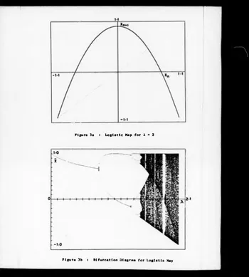
Figure 3e : Logistic Map for X - 2

Theorem. If f Is S-unlmodal then It has at most one stable

periodic orbit in [f(l),l].

We now consider the bifurcations of stsble periodic orbits

occurring in the logistic map.

1.2 Bifurcations of Stable Periodic Orbits

A graph of Equation 1.2 is shown in Figure 3a for the case

X - 2, together with the diagonal map Xq

+1

intersection of the graph with the diagonal represents a fixed point

of the mapping, the stability of this fixed point is determined by

the gradient of the slope at the point of intersection l.e.:

l> - | f'(Xo) |

M <

1

attracted to It. For W 1 the point becomes unstable, the case

W ■

1

The question of what occurs after X is Increased beyond the

critical value Xc , at which point Xq becomes unstable, is answered

by reference to the graph of f

2

graph intersects the diagonal in two places at which the slope is

less than unity for X > Xc [24). Thus exactly at the point at

which Xq becomes unstable two new stable fixed points are created,

this is an example of a pitchfork bifurcation.

As X is further increased, the period two fixed points

bifurcate in an analogous way to give a stable period 4 orbit, the

bifurcations continuing through period

8

some critical value X - X« is reached at which the stable orbit has

'bifurcated to infinity'. At this point the system is chaotic, the

-chaos persisting in the parameter range [X«», 2] except for parameter

'windows' in which stable periodic motion exists* Figure 3b shows

the bifurcation diagram of the logistic map, the first few pitchfork

bifurcations are clearly visible together with the large stable

period 3 window present in the chaotic regime.

The chaotic nature of the orbits lying to the right of the

period 3 window is indicated by the following theorem due to

Sarkovskil [10]:

Theorem. Order the integers as follows:

3 > 5 > 7 > 9 > ...

... > 2.3 > 2.5 -> 2.7 > ...

. .. > 2n.3 > 2n .5 > ...

... > . . . > 2 » > . . . > 8 * > 4 > 2 > 1

Then if f is unlmodal and has a point with period p, then it

has a point with period q Vq < p in the sense of the above

ordering.

Thus, after the point A

3

appears, the map will have a countable infinity of unstable periodic

orbits of every integer period. This result is related to a theorem

due to Li-Yorke which indicates that 'period 3 implies chaos' [15].

1.3 Felgenbaum Sequences

For a given value of A ■ X„ at which a 2n stable periodic cycle

has been created, the graph of:

2

ft f

1

f

2

viewed locally near these fixed points Is a rescaled copy of the

original mapping. This observation led Felgenbaum to consider

a renormallsatlon procedure for a general unlmodal mapping which

produced a universal scaling law for the parameters X„,

characterised by a universal constant

6

Denote by X„ the parameter value at which there Is a

bifurcation from period

2

2

( *n - *n-l ) -*•

6

-1

where

6

6

Stated another way:

Xn - X. + A

6

where X« Is the parameter value for which the bifurcations

accumulate and A Is a constant.

T h e above scaling law Is Independent of the particular mapping

used, exactly the same scaling applies to all unlmodal maps.

1.4 Lyapunov Exponents

T h e general definition of Lyapunov exponents for a flow was

given in the last chapter. Intuitively the exponents measure the

mean expansion rate of trajectories of a system. For 1-D discrete

maps there exists a single Lyapunov exponent which Is defined as

follows:

N

o ( X o ) - L l m i X In I df_ I . ...(1.4)

N+- N 1-1 I dx

4

where the xj are the i-th Iterates of the Initial condition Xq. The

exponent therefore measures the average slope of the map around an

orbit. Except for a set of measure zero the exponent is Independent

of the initial condition, xQ.

A negative value of o indicates an average slope less than

unity and corresponds to stable periodic behaviour, whilst the case

of o positive implies an average slope greater than unity and

corresponds to chaotic behaviour.

Numerically obtaining the graph of o as a function of A is

difficult due to the fact that stable period orbits are dense in

the parameter space, and hence the graph of a is extremely

complicated with an infinity of regions where a is negative

superimposed on the general upward trend of the curve with

increasing A [10]. Nevertheless, regions such as the stable period

3 window are clearly visible in numerical experiments of this type.

1.5 Probability Distributions

An invariant distribution for a mapping f is a function P(x)

with the property:

P ( . ) - f P < * ) , • • • ( 1 * 5 )

l.e. the function is mapped into Itself by f.

Ue call P(x) a probability distribution if:

/ P(x) dx - 1 #

A unique probability distribution Is singled out from the many

Invariant distributions for a given map by repeated Iteration of the

map. For the case of a stable periodic orbit of period n, P(x) will

be a set of n delta functions (each weighted by

1

values of the n fixed points of fn . In the general case of a

chaotic map we may find P(x) numerically by Iterating the functional

equation:

P(x) dx “ P(xj) dxi + P(*2)

or » « ) - P<»

1

2

1

6

( d f/dn) (df/do2 >

where xj and X

2

Equation 1*6 can be solved exactly for one case of a chaotic

logistic map. Considering the second fora of the logistic map with

X - 4 :

*n+l - 4*n d - * n ) . ••• d « 7 )

we make a change of variable:

« - (¿) .In

- 1

1

8

Inserting Equation 1.8 into Equation 1.7 yields a so-called 'tent

map':

»

0+1

- 1 2 i n 0 < < » . . . ( 1 . 9 )

1 2 ~ 2lo i < i n < 1

The probability distribution for the tent map is easily derived

from Equation 1.6: P(x) " 1.

Now, using the property: P(x) dx - P(x) dx, we obtain the

Invariant dlatrlbutlon for Equation 1.7*

-*

P(x) (x(l-x)) . ... (1.10)

X

The existence of a continuous probability distribution for a

map implies that the system is ergodic. In fact, the dynamics of

the logistic map for X - 4 are both mixing and ergodic.

Of particular Interest Is the existence of singularities In

P(x). These occur for x - 0, and x - 1, for the above case and are

due to the mapping of the maximum of the logistic curve (a point of

Infinite contraction) onto the points x -

1

0

fixed point). The 'singularity points' x ■ 1, 0, form the

boundaries of the chaotic motion In the Interval. For the case

X ■ 4 (or X - 2 for Equation 1.2) these points lie at the extremes

of the interval, as the parameter is decreased, the singularity

points move inwards and the chaotic motion is bounded in a smaller

Interval, this Is clearly visible In Figure 3b. At a certain

parameter value (X » 1.5436), the maximum Is mapped onto 3 points,

the last of which is an unstable fixed point, producing 3

singularities in the probability distribution. As X Is decreased a

little below this value, two disjoint regions are formed for P(x),

the region of chaos has therefore bifurcated into two regions. This

'period-doubling' bifurcation continues and accumulates on X«, in

fact the parameter values at which the bifurcations occur form a

Feigenbaum sequence and are characterised by the same 'Felgenbaum

constant'

6

-1.6 Summary

This section has dealt with the dynamics of 'unlmodal' maps

with particular reference to the logistic map. Many qualitative

features of the system are similar to those described for flows In

the last chapter, In particular, the period doubling cascade to

chaos Is also a common occurrence In continuous dynamical systems.

The main difference between the I-D systems described above

and the dynamics of flows Is that global attraction to a strange

attractor Is here replaced by singularities In the probabllllty

distribution of the map which form sharp boundaries for the chaotic

regions. Such bounding of chaotic regions by singularities Is also

found for a 2-dlmenslonal map to be described In Chapter 5. The

unlmodal maps are also unique In that a universal scaling Is

associated with their bifurcation properties, no such universality

Is apparent In continuous systems.

In the remainder of this chapter two examples of chaotic 2-D

discrete systems will be described.

2.0 Examples of 2-D Discrete Systems

2.1 The Hinon Map

Hinons map [16] Is defined by the equations:

«n+l - in +

1

2

*

0+1

where a and b are constants.

During one Iteration of the above, the mapping contracts area

by a factor |J| where:

-J - -b (2.2)

18

For x„ large, aolutlons of Equation 2.1 are unbounded, however,

for x„, yn , within some finite region of the origin, solutions

converge forwards an attractor.

Two fixed points of the mapping exist provided:

• > «„ - -(l-b)2 . ... (2.3)

4

one of these fixed points Is always unstable whilst the other Is

stable for 'a' In the Interval:

• o - - » - M 2 < • < 3 ( l - b ) 2 - • ! . . . . ( 2 . * )

4 4

For a > ax the fixed point la observed to undergo a cascade of

period doubling bifurcations until some accumulation point a» after

which a strange attractor appears to exist for 'a' In some finite

interval (a», a

2

2

orbits escape to Infinity.

Although the presence of a atrange attractor for a c (a», a

2

Is strongly Indicated by numerical Iterations of the equations

(typically, the chaotic motion Is seen to persist for 5 million

Iterates) It has not proved possible so far to prove the chaotic

nature of the H£non map In this region. In fact, Newhouse [15] has

suggested that the chaotic motion observed Is really the motion

near a very large period sink.

For the singular case b ■ 0, Equations 2.1 reduce to the

logistic sup for which chaotic motion Is known to exist, it could

-be argued chat the logistic map provides a good approximation to the

Hinon map along its unstable manifold, and hence that strange

attractors would be expected to exist for some range of 'a'a*

However, the link between the theory of the one dimensional system

and the Hinon map has not been made and the question of the

existence of strange attractors for the Hinon system remains an open

question.

The difficulty in proving chaotic motion for the Hinon map Is

related to the fact that the attracting region has a fold due to

the unstable manifolds folding back on themselves. Therefore, a

hyperbolic structure cannot be defined for the system as stable and

unstable manifolds will not In general Intersect transversely (a

'stable foliation' of the system does not exist).

This situation pertains also to the Duffing system considered

In the last chapter, the unstable manifolds of which have this

folding structure. Thus, the existence of a strange attractor for

the Duffing equations also remains an open question.

The constant area contraction property of the system indicates

that areas will be contracted down to one dimensional curves.

When the attracting region Is observed numerically, the attractor

Is seen to consist of an infinite number of concentric curves having

an apparently 'fractal' structure. The structure of the strange

attractor corresponds to the cross product of a line with a 'Cantor

set'.

The fractal dimension of the Hinon map has been numerically

determined to be: d * 1.202 for a ■ 1.2, b ■ 0.3, l.e. the

attractor 'almost fills' an area. Orbits on the attractor move