Analysis and processing of HRCT images of the lung for automatic segmentation and nodule detection

(1)

Analysis and processing of HRCT images of the lung for

automatic segmentation and nodule detection

A thesis

submitted in partial fulfilment

of the requirements for the degree

of

Master of Science

in

Computer Science and Software Engineering

at the

University of Canterbury

by

Huaqing Chen

_________________________________________________

Dr. Ramakrishnan Mukundan………Principal Supervisor Associate Professor, Department of Computer Science and Software Engineering,

University of Canterbury

Dr. Anthony Butler……….………Co-Supervisor Senior Radiologist, Department of Radiology, University of Otago

University of Canterbury

(2)

(3)

(4)

(5)

Abstract

(6)

Acknowledgments

First and foremost, I would like to thank my supervisor, Dr Ramakrishnan Mukundan, for providing me with such a wonderful and rewarding research experience: you encouraged me to study things I thought I would never study and see places I thought I would never see. Special thanks to Dr Anthony Butler and Dr Justin Hegarty for providing a large collection of anonymised HRCT images (including both test images and reference images), which have been valuable for this research. I would also like to thank them for the useful discussions we had, which provided important information about medical images. I am thankful to Frieda Looser from the Learning Skills Centre for doing grammar checking for this document. I would like to thank the Bioengineering Group of the University of Otago, Christchurch, for providing HRCT datasets for this project.

(7)

i

List of Figures

(11)

v

Figure 4.1 The flow chart of the lung segmentation method ... 27

Figure 4.2 HRCT lung image regions ... 28

Figure 4.3 Intensity difference of the three main regions ... 29

Figure 4.4 Process of flood fill (a) First seed point allocation (b) Second seed point allocation (c) Identification of the complete surrounding thorax region using flood fill ... 31

Figure 4.5 (a) Horizontal scan (b) Vertical scan... 32

Figure 4.6 Coarse lung regions ... 32

Figure 4.7 Air filled regions vary in size, location and shape ... 33

Figure 4.8 The statics of lung and trachea... 34

Figure 4.9 Labelled coarse lung regions ... 34

Figure 4.10 Connected components labelling ... 35

Figure 4.11 Trachea elimination procedure ... 36

Figure 4.12 Coarse lung regions with tracheas removed ... 37

Figure 4.13 Lung boundary information lost (a) Lung nodule locates on the lung boundary (b) Lung nodule pixels are affected by the flood fill process37 Figure 4.14 Horizontal and vertical mask [59] ... 38

Figure 4.15 (a) Lung regions after flood fill and CT background removal operations (b) Result of applying the dilation mask four times (c) Dilated lung regions shown by original pixel intensity ... 39

Figure 4.16 (a) dilation×1 (b) dilation×2 (c) dilation×3 (d) dilation×4 ... 39

Figure 4.17 Optimise lung boundary ... 40

Figure 4.18 (a) Edge peel ×1 (c) Edge peel ×2 (d) Edge peel ×3 (e) Edge peel ×441 Figure 5.1 Nodule candidates extraction ... 45

Figure 5.2 Lung segmentation with nodules indicated by squares (a) Original lung image (b) Segmented lung regions ... 47

Figure 5.3 α-images with nodule pixels indicated by squares (a) α-image without nodule information (b)-(e) images with nodule information (f) α-image without nodule information ... 47

Figure 5.4 α-images combined from α-range 1.77 to 1.94 ... 48

Figure 5.5 Nodule candidates with centroids marked ... 49

Figure 5.6 Centroid based filtering (a) Nodule candidates with centroids located outside are circled (b) Centroid based filtering result ... 50

(12)

vi

Figure 5.8 Intensity mean difference between nodules, veins and lung tissue... 51

Figure 5.9 Intensity based filtering (a) Nodule candidates with low intensity are circled (b) Intensity based filtering result ... 51

Figure 5.10 (a)-(e) Consecutive HRCT slices (i)-(v) Combined α-images processed by centroid and intensity based filtering processes... 52

Figure 5.11 Nodule pixel appearance on consecutive HRCT slices ... 54

Figure 5.12 Nodule candidates need to be kept (a) α-image shown in Figure 5.10(ii) (c) Combined α-image shown in Figure 5.10(iii) ... 55

Figure 5.13 Nodule candidates need to be removed (a) α-image shown in Figure 5.10(ii) (c) Combined α-image shown in Figure 5.10(iii) ... 55

Figure 5.14 Pre-identified nodules need to be kept (a) Combined α-image shown in Figure 5.10(ii) (b) Combined α-image shown in Figure 5.10(iii) (c) Combined α-image shown in Figure 5.10(iv) ... 56

Figure 5.15 Result of the step 1 process ... 57

Figure 5.16 Nodule candidates need to be kept (a) Result of the step 1 process (b) The next third combined α-image ... 57

Figure 5.17 Nodule candidates need to be removed (a) Result of the step 1 process (b) The next third combined α-image ... 58

Figure 5.18 Frequency based filtering (a) Nodule candidates need to be removed by the frequency based filtering are circled (b) Frequency based filtering result ... 58

Figure 5.19 Shape feature based nodule detection ... 59

Figure 5.20 Filtered nodule candidates labelled by numbers ... 60

Figure 5.21 Labelled nodule candidates enlargement ... 61

Figure 5.22 Minimum and maximum radii ... 62

Figure 5.23 Nodule radii for the detecting nodules (a)-(c) Original size nodules (1)-(3) Nodules with minimum and maximum radii indicated ... 62

Figure 5.24 Nodule areas for detecting nodules (1)-(3) Nodules with size in x and y directions indicated ... 63

Figure 5.25 Ratio difference between the three nodule shapes ... 65

Figure 5.26 Nodule detection (a) Filtered nodule candidates. (b) Detected nodules are highlighted ... 66

Figure 6.1 Lung segmentation results ... 69

(13)

vii

Figure 6.3 Image from upper lung portion (a) Original lung image (b) Lung segmentation result with restored bronchi region indicated (c) Manual

lung segmentation result with restored bronchi region indicated ... 75

Figure 6.4 Image from lower lung portion (a) Original lung image (b) Lung segmentation result (c) Manual lung segmentation result ... 76

Figure 6.5 Image from middle lung portion (a) Original lung image (b) Lung segmentation result with lost lung regions indicated (c) Manual lung segmentation result with lost lung regions indicated ... 76

Figure 6.6 Original lung image with high intensity vein indicated ... 78

Figure 6.7 Lung boundaries detected by: (a) Proposed method (b) Sobel operator with missed boundary indicated (c) Canny edge detector with missed boundary indicated (d) Holder exponent with missed boundary indicated... 78

Figure 7.1 Spherical shape nodule detection results ... 81

Figure 7.2 Star shape and quadrilateral shape nodule detection results ... 83

Figure 7.3 Irregular shape nodule detection results ... 85

Figure 7.4 Nodules attached to veins nodule detection results... 86

Figure 7.5 (a) Spherical shape nodule with large area ratio (b) Quadrilateral shape nodule with small radii ratio ... 90

Figure 7.6 The effect of nodule enlargement process on nodule size (a) Detection rate comparison (b) False positive rate comparison ... 92

Figure 7.7 The effect of the rule based filtering process on nodule size (a) Detection rate comparison (b) False positive rate comparison ... 93

Figure 7.8 The effect of the rule based filtering process on nodule shape (a) Detection rate comparison (b) False positive rate comparison ... 94

Figure 7.9 The effect of the rule based filtering process on nodule location (a) Detection rate comparison (b) False positive rate comparison ... 95

Figure 7.10 Lung image with a star shape nodule indicated ... 98

Figure 7.11 Type of intensity measures: (a) Sum Measure (b) Iso Measure (c) Maximum Measure (d) Inverse Minimum Measure ... 99

Figure 7.12 Error rate of the measures ... 100

Figure 7.13 Nodule indicated combined α-image with sum measure based on: (a) Multiple concentric windows (b) Multiple concentric discs ... 101

Figure 7.14 α-histograms: (a) Multiple concentric windows (b) Multiple concentric discs ... 102

(14)

viii

List of Tables

Table 5.1 Nodule radii ratio ranges for different nodule shapes ... 64

Table 5.2 Nodule area ratio ranges for different nodule shapes ... 64

Table 6.1 Performance metric measurement for upper lung portion images. .... 75

Table 6.2 Performance metric measurement for lower lung portion images. .... 76

Table 6.3 Performance metric measurement for middle lung portion images. .. 77

Table 6.4 Comparison with Sluimer et al.’s method. ... 77

Table 6.5 Comparison with Vinhais et al.’s method ... 77

Table 7.1 Experiment results based on different nodule sizes ... 88

Table 7.2 Experiment results based on different nodule shapes ... 89

Table 7.3 Experiment results based on different nodule locations ... 90

Table 7.4 Performance results of the proposed method ... 96

(15)

1

Chapter 1 Introduction

Medical image processing techniques can be used for diagnosis, treatment and research in medical imaging such as ultrasonography, High Resolution Computed Tomography (HRCT) and Magnetic Resonance Image (MRI). HRCT is the most commonly used diagnosis technique for the analysis of the lung regions and the number of HRCT evaluations of the lungs has been steadily increasing. Initially, HRCT images were only used by radiologists to diagnose patients’ disease symptoms [1]. The radiologists identify the disease symptoms by visually searching for the abnormal texture shown on the HRCT images. Recently, research began to focus more on analysing medical images by using Computer Aided Diagnosis (CAD) systems [2], where the aim is to help medical professionals identify the disease symptoms more accurately. The CAD systems help radiologists to characterise the distribution of the disease patterns found on the HRCT images [3] and make their final decisions more confidently. The research presented in this thesis describes techniques for lung segmentation and lung nodule detection. The lung segmentation technique is used to pre-process the lung image, and the lung nodule detection technique uses the pre-processed lung image for further nodule detection.

(16)

2

another fast method for the removal of the CT background using linear scans originating from border pixels. Connected components that represent parts of the trachea are removed by noting the separation of the mean and standard deviation of intensity values between the trachea and the lungs. The segmented lung images are further enhanced to restore the intensity values of the pixels on the bronchi and the lung boundary.

The nodule detection technique detects nodules existing on the segmented lung regions. Firstly, lung nodule candidates are defined as the regions of interest that possibly contain nodules, which are extracted by combining the pixels with similar intensity variation on the segmented lung regions. Then, extracted nodule candidates are filtered by a rule based filtering process. Finally, a shape descriptor is used to determine the shape features of the nodule candidates and compare them with the collected nodule shape features for identification. Instead of searching for a particular shape and large size lung disease symptom textures appearing on lung images, the proposed nodule detection technique is able to detect small size nodules by enlarging them for more accurate shape feature determination.

In this research, the majority of non-nodule information is eliminated by the following two processes:

 Segmenting lung regions from original lung images to get rid of the information located outside of the lung regions, such as bones and surrounding tissue regions.

 Processing the segmented lung regions from a set of consecutive HRCT slices to eliminate the unnecessary information located inside of the lung regions, such as veins and lung tissue.

1.1 Motivation

(17)

3

Most of the nodule detection techniques have problems of (1) detecting lung nodules only with a radiologist’s assistance, (2) detecting a small number of nodules, and (3) manually inputting data to complete the nodule detection process.

Lung images have a highly irregular intensity distribution, and their description with traditional methods is insufficient. Intensity based image analysis has been found to be useful in describing the pixel intensity variation and determining the overall image characteristics.

1.2 Objectives

This research aims to develop a generic model for lung segmentation and lung nodule detection which will segment the lung regions from lung images and detect the lung nodules with different shapes, sizes and locations.

For lung segmentation, the following objectives are considered:

 Separating the CT background, the lungs and the thorax region surrounding the lungs by grey-level thresholding.

 Using flood fill algorithm to effectively identify the thorax region. The seed point of the flood fill algorithm needs to be allocated automatically in the thorax region.

 Removing the CT background by using linear scans originating from border pixels.

 Removing airways based on noting the separation of the mean and standard deviation of intensity values between the airways and lungs.

 Restoring the intensity values of the pixels on the bronchi and lung boundary for further lung image enhancement.

For lung nodule detection, the following objectives are considered:

(18)

4

 Combining the pixels that have the same intensity as the nodule pixels to extract suspected nodules.

 Filtering the suspected nodules based on comparing their characteristics with nodules.

 Determining the shape features of the suspected nodules.

 Identifying nodules by comparing the shape feature of the suspected nodules with the shape feature of nodules.

1.3 Thesis Overview

The rest of this thesis is organised as follows:

 Chapter 2 gives a brief interpretation of HRCT lung imaging and the literature review of lung image processing including lung segmentation and lung nodule detection.

 Chapter 3 reviews the α-image decomposition based image analysis technique, which is used for processing highly irregular intensity distribution of lung images.

 Chapter 4 describes the development of the lung segmentation technique that pre-processes the lung image for further accurate nodule detection use.  Chapter 5 describes the development of the lung nodule detection

technique, which identifies nodules based on shape feature comparison.  Chapter 6 presents and analyses the results of the lung segmentation.

 Chapter 7 presents and analyses the results of the lung nodule detection and evaluates some technique parameters.

(19)

5

1.4 Publication

The following paper was presented at the Otago Medical School, Christchurch:  H. Chen, R.Mukundan, A. Butler, K.Hart. “A Multifractal Formulism for

Segmenting HRCT Images of the lung”, Oral presentation, Communicating Bioengineering Research, The Centre for Bioengineering, University of Otago, Christchurch, 10November 2010.

The following paper was published in the Twenty-sixth International Conference on Image and Vision Computing New Zealand:

 H. Chen, R. Mukundan, A. Butler. “Automatic Lung Segmentation in HRCT Images”, International Confernce on Image and Vision Computing,

(20)

(21)

6

Chapter 2 Background

In this chapter, a brief background of lung anatomy, HRCT imaging and nodule characterisation is reviewed, followed by a description of lung image processing that subsequent chapters will be based on.

Section 2.1 reviews the domain knowledge of lung anatomy, HRCT imaging and nodule characterisation. Section 2.2 gives an overview of the related work on lung image processing including lung segmentation and lung nodule detection.

2.1 HRCT Lung Images Interpretation

Detailed understanding of lung anatomy, HRCT imaging and nodule characterisation is a necessary step for successful image interpretation. The way lung anatomy appears on HRCT images and radiologists interpret images are explained in this section. Section 2.1.1 describes the anatomical features of the lung, as well as the different lung regions. Section 2.1.2 introduces the structure of HRCT lung images and also explains the components of the HRCT images. Section 2.1.3 presents some common lung nodules and discusses their features.

2.1.1 Lung Anatomy

(22)

7

[image:22.595.166.430.450.652.2]

connective tissue that holds up the lung structure. The alveoli and bronchioles are connected to each other as a bronchial tree and run alongside each other [4].

Figure 2.1 Bronchi, bronchial tree, and lungs. [4]

The lung regions can be further divided into three different regions: Apical, Middle and Basal [5]. In Figure 2.2, the lung regions are categorised into three regions. The division occurs along the axial plane of the human body.

Figure 2.2 Further division of the lung regions [5]

(23)

8

2.1.2 Lung HRCT Images

HRCT scanners generate a three dimensional view of the imaged organs in the axial section of the human lung, as shown in Figure 2.3(a). Each lung HRCT image is a two dimensional view of the imaged organs with sub-millimetre resolution. It provides high spatial and high temporal resolution for the pulmonary structures and surrounding anatomy so the detailed information of the imaged organs and lung nodules can be clearly seen from the images. Continuous lung HRCT images shown in Figure 2.3(b) are able to produce 3D volume data and enable precise imaged anatomy visualisation and disease pattern visualisation.

Figure 2.3 (a) Human lung (b) Continuous HRCT images (c) Normal HRCT slice [6]

In order to differentiate the HRCT images belonging to different lung regions, hilum is used as an anatomical landmark. Images located above the hilum belong to the Apical region, images containing the hilum belong to the Middle region, and images located below the hilum belong to the Basal region. Figure 2.4 shows a lung image belonging to the Middle region.

(24)

9

Figure 2.4 Trachea splits, top of the lung [5]

2.1.3 Lung Nodule Characterisation

Lung nodules usually appear as small regions with spherical, ellipsoidal or star shapes [7] [8] in the HRCT lung images. However, in practice, most of nodules are not perfectly spherical but exhibit very large variations in shapes, sizes and intensities, as illustrated in Figure 2.5.

(a) (c)

(b) (d)

Figure 2.5 Illustration of different types of nodules: (a) Nodule attached to lung boundary (b) Vascularised nodules (c) Solid nodules (d) GGO nodules [9]

(25)

10

Figure 2.6 Cancer and non-cancer nodules [11]

2.2 Literature Review of Lung Image Processing Methods

Lung image processing is a fundamental step for most lung image analysis applications. HRCT images have been used for applications such as lung parenchyma density analysis [12], [13], airway analysis [14], and disease detection [15] [16]. In this research, lung HRCT images are used for nodule detection and analysis. Most of the CAD systems consist of two stages, the first of which is the lung segmentation, and the second is the characterisation of disease pattern.

In this section, common lung image processing techniques are explained. Section 2.2.1 gives a brief overview of current lung segmentation techniques. Section 2.2.2 reviews the relevant literature of nodule detection techniques.

2.2.1 Lung Segmentation

(26)

11 Manual Lung Segmentation

A number of successful manual techniques have been presented by several researchers: Denison et al. [17] used the manual lung boundary tracking method to estimate regional gas and tissue volumes in lungs; Kemerink et al. [18] developed a manually corrected border-tracing algorithm to segment the lung regions; Hedlund [19] introduced 3D region growing with seed points manually specified for segmenting the lungs; Kalender et al. [20] obtained anterior and posterior junction lines manually to separate the left and right lungs in cases where the edge contrast is reduced by the volume averaging.

Automatic Lung Segmentation

Several automatic techniques have been developed by a number of groups as manual segmentation became time consuming: Shojaii et al. [21] provided a lung segmentation technique based on a watershed transform and rolling ball filter. The watershed transform is used to find the lung boundaries and the rolling ball filter is used to smooth lung contours. Most lungs appear as dark regions in HRCT images and they are surrounded by the high density surrounding thorax region. The majority of the lung segmentation frameworks are based on grey-level thresholding. Figure 2.7 shows the lung segmentation result of Shojaii et al.’s method.

(a) (b) (c) (d)

Figure 2.7 (a) Original HRCT image (b) Segmented lung boundary (c) Smoothed lung boundary (d) Segmented lung regions [21]

(27)

12

shown that this refinement step introduces a significant improvement in segmentation accuracy compared to a standard segmentation-by-registration approach. The method of Vinhais et al [23] consists of an initial step to segment the patient from the background of the image, an extraction step to identify the large airways, decomposing the lung parenchyma, and a final segmentation step to extract the lung regions. Figure 2.8 gives the lung segmentation result of Vinhais et al.’s method.

(a) (b) (c) (d)

Figure 2.8 (a) Constrained dilation of air voxels (b) Interior cavities elimination (c) Region of interest (d) Surface rending of the segmented lung regions [23]

Tseng et al. [24], developed a lung segmentation technique which is able to determine the threshold for each individual CT image and segment the lung regions automatically. Some output examples of Tseng’s method are shown in Figure 2.9.

(a) (b) (c) (d)

(28)

13

The shortcoming of the grey-level thresholding technique is it does not perform well if there is an intensity overlapping between the lung regions and a surrounding thorax region. Hu et al. [25] presented a way of comparing the result generated by the manual and the automatic segmentation technique. They use mean, RMS and maximum distance between the automatically extracted lung boundary and manually extracted lung boundary to assess the accuracy of the lung boundary position. According to their boundary difference calculation, they found that the greatest difference between the manually segmented lung boundary and automatically segmented lung boundary occurs on the lung boundaries near to the mediastinum.

The main advantage of lung segmentation techniques is that they minimise the nodule searching area for lung nodule detection.

2.2.2 Lung Nodule Detection

Lung nodule detection is the process of determining whether nodule patterns appear on the HRCT lung image and identifying the location of the nodules. Dr Giger and Dr Doi from the University of Chicago have shown that it is feasible for lung nodules to be automatically extracted from the X-ray radiography based on their features [26]-[27]. Currently, researchers have developed a number of lung nodule detection methods which can be classified as: classification based nodule detection (includes feature based nodule detection), template matching based nodule detection and clustering based nodule detection.

Classification Based Nodule Detection

(29)

14

discriminant analysis (LDA) and Bayesian classifier. Those machine learning methods are used to reduce the false positives in the lung nodule detection.

Suzuki et al. [28]-[29] developed a massive training ANN to detect both benign and malignant nodule patterns; Boroczky et al. [30] trained a SVM classifier on the subset of optimal features to identify the nodule candidates as nodule or non-nodule; Ginneken [31] implemented linear and non-linear k-NN regressions and SVM to predict the unseen nodule feature vector. Figure 2.10 gives three example nodules segmented by Ginneken’s method.

[image:29.595.173.425.285.540.2]

(a) (b) (c)

Figure 2.10 (a) CT data, axial or coronal sections zoomed in on the nodule with a lung window level, W/L = 1400/-600 HU (b) Truth (c) Segmented lung regions [31]

(30)

15

counterparts; Klik et al. [34] also implemented multiple classifiers to classify benign sub-pleural nodules. They used k-NN, Parzen, LDA and quadratic discriminant to detect lung nodules, and they found LDA performed slightly better than its counterparts. Lin et al. [35] proposed a neural network model, Convolution Neural Network (CNN) architecture, to extract suitable features from chest radiographs and classify the nodules among the suspect nodule area (SNAs).

Feature based nodule detection uses the extracted nodule features to identify nodules. Most features relate to shape, size and intensity on the premise that nodules tend to be spherical and are of greater diameter, and they also have higher intensities than those of lung parenchyma. Kim et al. [36] developed a texture based classifier to classify the true nodules from nodule candidates based on features like shape, size, correlation coefficient and standard deviation;

Template matching Based Nodule Detection

Template matching based nodule detection is based on a simple model that simulates read nodules are the reference image. Several successful template matching based nodule detection techniques have been presented by several authors: Lee et al. [37] applied both semicircular matching and genetic algorithm to identify initial nodule candidates and attenuation, shape, and gradient feature rules to reduce false positives in the nodule detection; Figure 2.11 shows the eliminated and overlooked false positive candidates processed by Lee’s method.

Figure 2.11 White arrows indicate false positive candidates removed by elimination process. A black arrow indicates a false positive candidate that remained after the elimination process. A

(31)

16

Dehmeshki et al [38] proposed a similar method with Lee [37], the only difference they made is they added a Shape Index (SI) parameter to the fitness Equation of the generic algorithm, which helps to improve the nodule detection result; Shigemoto et al. [39] proposed a template matching method base on using defined nodule and vein models. The problem with this method is that the pre-defined models are not applicable for all types of lung nodules and it is unable to describe nodules with irregular surface and small size.

The weakness of the template matching based methods is it requires prior knowledge expressed by functions like Gabor or Gaussian [40] to pre-define all the different templates. However, it is difficult to pre-design the functions to accurately represent the various nodules.

Clustering Based Nodule Detection

(32)

[image:32.595.145.451.101.360.2]

17

Figure 2.12 Architecture of the four-fuzzy neural network [41]

Kanazawa at al. [42] described a diagnosis rule based on fuzzy clustering, which is used to partition the histogram of pixels within the lung fields into three regions: “airway region”, “blood vein region”, and “tumour region”. They finally classify nodules and veins based on using similar features in a heuristic rule-based approach; Kawata et al. [43] proposed a linear discriminant classification method based on k-means clustering using benign and malignant lung nodule datasets based on topological histogram features.

(33)

18

Chapter 3 Processing of HRCT Images

The intensity distribution in biomedical images is highly irregular and does not often permit a direct definition of shape parameters using geometrical descriptors. The Holder exponent [44], [45] is used in this research for resolving local densities variation in HRCT lung images. This chapter gives an overview of image representation followed by measuring the image intensity distribution based on the Holder exponent.

Section 3.1 gives a brief overview of image representation. Section 3.2 presents the Holder exponent for quantifying local density variation, and four different measures are discussed for the Holder exponent estimation. Section 3.3 discusses α-image generation and usage.

3.1 Image Representation

Each digital image is combined with a different number of pixels, each pixel having a particular location and intensity, as shown in Figure 3.1. As mentioned in Section 2.1.2 the HRCT lung images used in this research are in greyscale intensity and with 16 bit colour depth. So we consider 65536 levels of grey, from 0 (black) through to 65535 (white). Image pixels can be viewed from the enlarged lung junction image with size M×N in Figure 3.1, the location of each pixel is given by the co-ordinate (m, n) and intensity value at that pixel is g(m, n).

(34)

19

Figure 3.1 Enlarged lung junction image

The whole image can be represented as a 2D matrix with M rows and N columns:

g(m, n) =

(0, 0) (0, 1) … … (0, − 1)

(1, 1) (1, 1) … … (1, − 1)

⋮ … ⋱ … ⋮

( − 1, 0) ( − 1, 1) … … ( − 1, − 1)

3.2 H

o

lder exponent

α

The Holder exponent α [44] [47] [48] [49] [50] represents the degree of intensity variation at each pixel position in the image. It is estimated for each pixel (m, n) as the slope of the linear regression line of the plot of log ( , ) versus log , for ε is the increasing size of the measure neighbourhood centred around the pixel (m, n).

µε(m, n) is the amount of intensity measured in the area. α-value computation is

reflected by the local behaviour of a measure µε(m, n), so choosing an appropriate

measure is important for accurate α-value computation.

Some commonly used measures µε(m, n), such as Sum measure, Iso measure,

Maximum intensity measure and Inverse minimum measure for multi-fractal based analysis are based on pixel intensity, and introduced by Jacques Lévy Véhel and Pascal Mignot [51], and are defined by Nilsson [48] as follows:

: _{( , )} = ( , )

( , )∈

(3.1) y

M-1

x

0 1 2 3 N-1

(35)

20

: _{( , )}= #{( , )| ( , ) ≡ ( , ), ( , ) ∈ Ω} (3.2)

: _{( , )}= max

( , )∈ ( , ) (3.3)

: _{( , )} = 1 − min

( , )∈ ( , ) (3.4)

In the above Equations, g(k, l) represents the greyscale intensity value at pixel

(m, n), ε is the size of the measure neighbourhood, and Ω is the set of all pixels

within the measure neighbourhood.

In this research, we choose to use Sum measure for α-value estimation. Those four different measures are described in detail in Section 3.2.1-3.2.4. The comparative analysis of the four intensity measures is presented in Section 7.3.1.

3.2.1 Sum Measure

Sum measure is defined as the sum of the intensity value within a local neighbourhood. The local neighbourhood is usually in disc shape, square shape or diamond shape, and those shapes are known as neighbourhood shapes. Nilsson [48] summarised that different neighbourhood shapes can affect the estimation of the intensity measure µε(m, n).

In this section, we discuss the Sum measure based on disc and square neighbourhood shapes; they are known as Multiple concentric discs and Multiple concentric windows:

 Multiple concentric discs: A measure p() in a disc of radius  at centre

point p.

 Multiple concentric windows: A measure p(r) in a square of size r at centre

point p.

(36)

21 Multiple concentric discs and windows

In the Multiple concentric discs, we denote the measure function as p(), and 

represents the radius size of the disc region centred at a pixel p in which the measure is defined (see Figure 3.2(a)). The p() stands for the intensity sum of the

pixels inside the disc region with radius . In Multiple concentric windows, r represents the size of the square centred as pixel p in which the measure is defined in Figure 3.2(b). The p(r) stands for the intensity sum of the pixels inside the

square region.

(a) (b)

Figure 3.2 Sum measure window shapes (a) Multiple concentric discs (b) Multiple concentric windows

In the Multiple concentric discs, the exponent at p is the term that shows how p()

scales with  according to the power law in Equation 3.5. The exponent at p in Equation 3.6 shows how p(r) scales with r for the Multiple concentric windows.

( ) = (3.5)

(r) =

(3.6)

C is a constant in the above two Equations. The term α is an important term in

characterising the variation of intensity. With the enlargement of the neighbourhood size, m denotes the total number of discs used in the computation of α in the Equation 3.7, and n denotes the total number of squares used for α computation in the Equation 3.8.

 = , = 0, 1, 2, … , . (3.7)

(37)

22

= 2 + 1, = 0, 1, 2, … , . (3.8)

Because of the neighbourhood shape difference between the Multiple concentric discs and the Multiple concentric windows, there is a difference in pixel increment. Figure 3.3 shows the neighbourhood size () for the Multiple concentric discs increases one pixel at a time. Figure 3.4 illustrates the Multiple concentric windows have a neighbourhood size (r) which increases two pixels each time. The exponent α in the Equations 3.5 and 3.6 also establishes a mapping from the original image

to an α-image, which is introduced in Section 3.3.

(a)  = 1 (b)  = 2 (c)  = 3 (d)  = 4

Figure 3.3 Neighbourhoods of  = 1, 2, 3, 4 respectively, for the centre pixel p [52]

(a) r = 1 (b) r = 3 (c) r = 5 (d) r = 7

Figure 3.4 Neighbourhoods of r = 1, 3, 5, 7 respectively, for the centre pixel p [52]

As the  value and r value for both Multiple concentric discs and Multiple concentric windows increase, the value of α at each pixel is estimated as the slope of the linear regression line through points on a log-log plot where log() and log(r) are plotted along the x-axis, and log(µp) along the y-axis, as shown in Figure 3.5(a)

(38)

23

(a) (b)

Figure 3.5 Linear regression lines for: (a) Multiple concentric discs (b) Multiple concentric windows

3.2.2 Iso Measure

As seen in Equation 3.2, the Iso measure counts the number of pixels which have the same intensity value with the centred pixel (m, n) in a neighbourhood. The counted number of pixels is the measure µr(m, n).

3.2.3 Maximum Measure

Equation 3.3 defines the measure µr(m, n) to be equal to the intensity of the

pixel with the greatest intensity in a neighbourhood. The greatest intensity value of pixel (m, n) is the measure µr(m, n).

3.2.4 Inverse Minimum Measure

In the Inverse Minimum measure, the µr(m, n) is the amount of measure in a

(39)

24

3.3 Decomposition of an

α

-image

α-image is represented by a number of pixels, which have similar Holder exponent. It is used to show the pixels on an image that have similar degree of intensity variation, such as the pixels on object edges.

3.3.1 The α-image

Once α-values are calculated for each pixel in the original image, the α-image with the same size as the original image can be created. A 512×512 lung image has 262144 (512×512) α-values, which are sorted from minimum (αmin) to maximum

(αmax). The intensity of each pixel in the α-image is set to represent the α-value of

the corresponding pixel in the original image. In order to enhance the contrast of the α-image and see the brightest and darkest points which lie around the areas of strongest singularity, we display α-values in the full range [0, 1]. Figure 3.6 illustrates both the HRCT lung image and its α-image. Figure 3.6(b) shows that the pixels on the lung boundary have a similar degree of intensity variation, so α-images are also able to show object edges. Dawei et al. [53] used the Holder exponent for medical CT image edge detection, and edge detection result is shown by α-image.

(a) (b)

(40)

25

3.3.2 Thresholding the α-image

The sorted α-values are further subdivided into n discrete intervals α1, α2, α3, … ,

αn. Each interval αk is defined as follows:

= + ( − 1)∆ _, = 1, 2, … , . (3.9)

∆ = ( − )/ (3.10)

We choose n = 100 and for each sub-range k we threshold the α-image by considering only pixels with α-value in range ≤ < ( + ∆ ). We can then obtain the α-image by assigning the value 1 to these pixels, and 0 to all others. The α-image shows the pixels with α-values belonging to the same interval of [αk,

αk+1], and those pixels have similar intensity variation [48] [49] [50]. The number

of pixels belonging to each α-interval is counted, and most of the pixels have a Sum measure calculated α-value around value 2.0, as shown in Figure 3.7.

Figure 3.7 Image α-histogram

(41)

26

Chapter 4 Lung Segmentation

In this chapter, a method is proposed to segment lung regions automatically from HRCT lung images. According to the region based intensity characterisation, the lung image can be considered as consisting primarily of three regions: the CT background, the lungs, and the thorax region surrounding the lungs. This method based on flood fill algorithm [54] is used to effectively identify the surrounding thorax region, as well as the CT background. This step facilitates the use of another fast method for the removal of the CT background using linear scans originating from border pixels. Connected components that represent parts of the trachea are removed by noting the separation of the mean and standard deviation of intensity values between the trachea and the lungs. The segmented lung images are further enhanced to restore the intensity values of the pixels on the bronchi and the lung boundary.

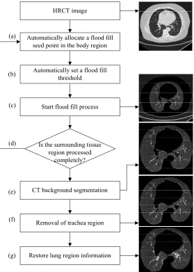
Figure 4.1 describes the structure of the proposed method, which consists of seven steps. An outline of these steps is given below.

a) Using a partitioning of the HRCT lung image into 16x16 boxes, a seed point position for the flood fill algorithm is automatically found in the body region. b) The flood fill process is initiated with a pre-specified threshold value.

c) The flood fill method visits all pixels in a connected component of the body region.

(42)

27

flood fill seed point is automatically allocated in the unprocessed surrounding thorax region and the flood fill process will start again.

e) The region corresponding to the CT background is now removed using an iterative algorithm.

f) Non-lung connected components are removed from the extracted coarse lung regions based on their pixel intensity mean and deviation.

g) Lung regions and the airway region can be distinguished by their pixel intensity difference. A 3×3 horizontal and vertical dilation mask is applied to recover the lung information lost during the flood fill process.

HRCT image

Automatically allocate a flood fill seed point in the body region

Automatically set a flood fill threshold

Start flood fill process

Is the surrounding tissue region processed

completely?

CT background segmentation

Removal of trachea region

Restore lung region information (a)

(b)

(c)

(d)

(e)

(f)

[image:42.595.162.441.310.701.2]

(g)

(43)

28

Section 4.1-4.5 presents the proposed method based on well defined intensity characteristics of different regions of HRCT images, and use flood fill, linear scan and morphological operations to identify the exact lung regions. Section 4.1 describes the method for separating the lung background, the body tissue region surrounding the lungs and the lung regions. Section 4.2 describes a method for flood fill seed point allocation. Section 4.3 provides an overview of CT background segmentation by using linear scan method on the flood fill processed lung image. Section 4.4 presents a method of eliminating lung airways from CT lung images. Finally, lost lung region information is restored in Section 4.5.

4.1 Region Separation

In an average sense, the intensity values around a pixel in an HRCT image can be roughly categorised to three regions, as seen in Figure 4.2: (1) the CT background, (2) the body tissue surrounding lungs and (3) the lung regions. In healthy HRCT images, the intensity of the body tissue surrounding lung regions is higher than the intensity of the CT background and the lung regions. Our method takes advantage of this separation of intensity values, and uses the flood fill method to first identify the pixels corresponding to tissue in the thorax surrounding the lung.

Figure 4.2 HRCT lung image regions

The flood fill method finds connected regions based on some similarity metric, and is used mostly in filling areas with colour in graphics programs [55]. In this proposed method, the flood fill method starts from a pixel that is called the seed

CT Background

Body Tissue

(44)

29

point, and looks for all the pixels in the array which are connected to the seed point. Any pixel connected to the seed point will be flagged if it has similar intensity with the seed point. The flood fill algorithm is recursively processed until all the connected pixels with similar intensity are processed. The flood fill algorithm pseudo code is given in Appendix A.1. Once this process is complete, the region outside this segment can be identified as the CT background region, and the region inside this segment can be identified as lung regions. The CT background region can be easily identified using a fast linear scan from each border pixel.

Figure 4.3 shows the pixel intensity mean difference between the lung regions, body tissue region, and the CT background, computed from several HRCT image slices. The pixel intensity values range from 0 to 65535. Figure 4.3 also suggests that a threshold of T1 = 15000 would be adequate to initiate a recursive flood-fill in

the body tissue region. It is feasible to separate the body tissue region with the lung regions and the CT background region by using the threshold T1 = 15000. The main

task here is to identify a seed pixel in the region, and also to make sure that all possibly disjoint, sections of this region are visited by the algorithm.

Figure 4.3 Intensity difference of the three main regions

4.2 Automatic Seed Point Selection

As seen in the previous section, the body tissue region is located in between the CT background and the lung regions in HRCT lung images. Implementing the flood fill method in the body tissue region can therefore separate the CT

0 20000 40000 60000 80000

0 5 10 15 20

R egi o n In te n si ty Slice No

(45)

30

background and the lung regions. The seed point is defined as the point with the maximum intensity within a neighbourhood of 16×16 pixels having intensity values in the upper region of Figure 4.3. A 16x16 window is found to adequately characterise the nearly uniform distribution of intensities in a neighbourhood, and it also provides the average intensity within the window. Increasing the window size further increases the error in describing uniform distributions, while reducing the window size makes it more sensitive to intensity variations. The HRCT image is therefore divided into 16×16 cells Rij. where i, j = 1,…,32, and the average

intensity rij in each cell is computed. Cells with average intensity greater than T2 =

45000 contain only pixels belonging to the surrounding thorax region. We select the cell G with the maximum average intensity g = maxij(rij), and define the seed

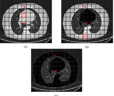
point as the pixel with the highest intensity in G. The previous steps are guaranteed to provide a cell in the body tissue region, and a seed point in that region (see Figure 4.4(a)). A recursive 4-connected flood fill algorithm using the threshold T1

visits an entire connected component within this region (see Figure 4.4(b)). All visited pixels and cells are marked, and the whole process is repeated if another component of unmarked cells with an average intensity greater than T2 exists. In

Figure 4.4(a), such disjoint components exist because of the anterior and posterior junctions (indicated by arrows). So, checking for the completeness of the flood fill process is an essential step for lung segmentation.

(46)

31

(a) (b)

[image:46.595.109.491.110.433.2]

(c)

Figure 4.4 Process of flood fill (a) First seed point allocation (b) Second seed point allocation (c) Identification of the complete surrounding thorax region using flood fill

4.3 CT Background Segmentation

(47)

32

vertical scan is represented by big-O notation. The size of the image is N×N, so the scan process requires O(N×N) time to execute.

(a) (b)

Figure 4.5 (a) Horizontal scan (b) Vertical scan

Figure 4.6 shows the coarse lung regions with the exterior of the body tissue region removed. Airways (trachea and bronchi) and lung regions are left over in the coarse lung regions image.

Figure 4.6 Coarse lung regions

4.4 Removal of Trachea Region

A number of authors have developed techniques for detecting lung airways from CT lung images [56]-[57]. In [25], Hu et al. used a slice-by-slice region growing method to remove airways and used the airway's location on the current CT slice to estimate the airway’s location on the next slice. However, the slice-by-slice region

Airways

(48)

33

growing method is not capable of segmenting the airways on some transverse slices [58].

In our method, we consider specific characteristics of the intensity distribution within the lung regions to identify and remove image segments that correspond to the airways. The images shown in Figure 4.7 have two things in common. Firstly, the trachea region has lower pixel intensity than the lung regions. Secondly, the presence of veins in the lung regions makes the lung regions vary in pixel intensity. So the lung regions have higher pixel intensity mean and deviation than the airway region.

Figure 4.7 Air filled regions vary in size, location and shape

(49)

[image:49.595.214.383.486.643.2]

34

Figure 4.8 The statics of lung and trachea

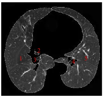
Each connected component in Figure 4.6 is labelled with a positive number, as shown in Figure 4.9. The labelled connected components are further processed to determine its shape and size. In our case, we will also need to calculate the pixel intensity mean and deviation for each connected component. If a specific connected component belongs to the trachea region according to its pixel intensity mean and deviation, this region will be discarded. Figure 4.8 suggests that the thresholds of trachea mean Tm = 20000 and trachea deviation Td = 50000 would be adequate to

remove the trachea region. A labelled connected component has to be removed if it has intensity mean < Tm, or intensity deviation < Td.

Figure 4.9 Labelled coarse lung regions

Labelling the connected components is done by two steps, which are seed image generation and label image generation. Both steps are performed on the coarse lung regions image (see Figure 4.6).

0 12000 24000 36000 48000 60000 72000

1 2 3 4 5 6 7 8 9 10 11 12 13 14 15 16 17 18 19 20

In

te

n

si

ty

Slide No

Trachea Mean Lung Mean Trachea Deviation Lung Deviation

1 2

(50)

35

a) Seed image generation: Seed image is generated by assigning two different numbers to non-background (non-black pixels) and background (black pixels) pixels as seen in Figure 4.9. The non-background pixels are assigned with number 1, and the background pixels are assigned with number 0. The number 1 and 0 are only used to differentiate the background pixels and non-background pixels.

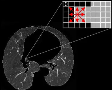
[image:50.595.205.391.427.577.2]

b) Label image generation: Label image is generated by assigning different label numbers to the connected components with pixels numbered by 1 on the seed image. In Figure 4.10, the grey cells in the enlarged window represent the non-background pixels, and the black cells represent the background pixels. The number labelling process scans the seed image pixel by pixel. Once any non-background pixel is scanned, all its connected non-background pixels in eight directions are assigned with a label number. The label number increases as more and more connected components are scanned. Labelled connected components are easy to be extracted and analysed by using its label number.

Figure 4.10 Connected components labelling

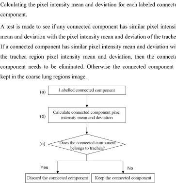
Each labelled connected component in Figure 4.9 can be picked out for determining its pixel intensity mean and deviation. Decisions can be made to either keep or discard the connected components on the coarse lung regions image. Figure 4.11 outlines the procedure of eliminating trachea regions from labelled coarse lung regions image, which is represented in three steps:

(51)

36

a) Each labelled connected component in the Figure 4.9 is picked out based on its label number.

b) Calculating the pixel intensity mean and deviation for each labeled connected component.

[image:51.595.128.491.151.529.2]

c) A test is made to see if any connected component has similar pixel intensity mean and deviation with the pixel intensity mean and deviation of the trachea. If a connected component has similar pixel intensity mean and deviation with the trachea region pixel intensity mean and deviation, then the connected component needs to be eliminated. Otherwise the connected component is kept in the coarse lung regions image.

Figure 4.11 Trachea elimination procedure

[image:51.595.186.449.326.532.2]

(52)

37

Figure 4.12 Coarse lung regions with tracheas removed

4.5 Restoring Lung Regions Data

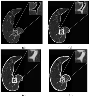
Bronchial walls, veins and nodules have generally higher intensity compared to the average lung regions and if they are near the boundary of the lung regions they will most likely get removed by the flood fill process. Figure 4.13(a) shows a lung nodule located on the lung boundary (indicated by a red arrow). In Figure 4.13(b), the lung nodule is lost after the flood fill process. Restoring the lost pixel information within the lung boundary is important for proper segmentation. We propose a method below for accurate reconstruction of the lung image region.

(a) (b)

Figure 4.13 Lung boundary information lost (a) Lung nodule locates on the lung boundary (b) Lung nodule pixels are affected by the flood fill process

(53)

38

4.5.1 Morphological Dilation

In greyscale morphology, the operation of dilation is used for region growing. This operation also closes holes and gaps within the region. Dilation makes an object larger by adding pixels around its edges [59]. The four most basic operations in mathematical morphology are dilation, erosion, opening and closing, and their corresponding effects are illustrated in Appendix A.2. Figure 4.14 shows four 3×3 dilation masks.

Vertical mask Horizontal mask

0 1 0 0 0 0

0 1 0 1 1 1

0 1 0 0 0 0

Horizontal and Vertical masks

0 1 0 1 1 1

1 1 1 1 1 1

[image:53.595.221.379.270.378.2]

0 1 0 1 1 1

Figure 4.14 Horizontal and vertical mask [59]

In order to close the lung gaps completely, we convolve the image with the dilation mask 4 times. Four times of dilation is reasonable enough to close up common size lung gaps although more dilation times are still feasible. However, increasing dilation times causes longer lung segmentation processing times. It also increases the amount of noise, which affects the segmentation accuracy.

(54)

39

(a) (b) (c)

Figure 4.15 (a) Lung regions after flood fill and CT background removal operations (b) Result of applying the dilation mask four times (c) Dilated lung regions shown by original pixel intensity

Figure 4.16 shows the result of the above sequence of operations when the image is dilated only once, twice, three and four times. A four-step dilation is used primarily to close the gaps represented by the bronchi.

(a) (b)

[image:54.595.151.442.395.709.2]

(c) (d)

(55)

40

4.5.2 Lung Boundary Enhancement

In Figure 4.17, the grey cells in the middle of the enlarged window represent the pixels from the body tissue region which were copied from the original image to the lung boundary. The cells marked with numbers are the labelled pixels in the lung regions and the black cells correspond to the background pixels. A scan-line algorithm is used to find the edge pixels which are adjacent to the black background pixels. Every edge pixel has a background pixel included in its eight neighbouring pixels and is also not part of the lung regions. Each scan-line strips off edge pixels found on it by setting their pixel intensity to zero. Repeating the process four times removes the four-pixel wide border introduced by the dilation operation.

Figure 4.17 Optimise lung boundary

The results of the edge peeling process for our sample image are shown Figure 4.18(a)-(d). In Figure 4.18(d), the border containing pixels from body tissue is completely eliminated. Note also the interior of the lung regions now contains the original pixel intensities.

1 1 1 1 1 1 1 1

(56)

41

(a) (b) (c) (d)

Figure 4.18 (a) Edge peel ×1 (c) Edge peel ×2 (d) Edge peel ×3 (e) Edge peel ×4

4.6 Summary

The proposed lung regions segmentation technique is based on flood fill and morphological operations to effectively segment lung regions of varying size, shape and location from HRCT images. Using the statistical characteristics of the intensity distribution, it is possible to easily distinguish, the lung and the airway.

The advantages and the limitations of the lung regions segmentation technique are listed as follows:

Advantages of the proposed technique

 The method is fully automatic; it does not require manual input of seed points or interactive selection of regions.

 The method provides accurate segmentation of the lung regions, and effectively removes the trachea regions and the surrounding region of the thorax.

 The pixel intensity values within the interior of the lung regions after segmentation are the same as the original image.

Limitations of the proposed technique

(57)

42

Chapter 5 Lung Nodules Detection

The previous chapter described the lung segmentation technique for segmenting lung regions, which minimises the nodule detecting area on lung images. However, the existence of the non-nodule noise information inside the lung regions still affects the nodule detection accuracy. In this chapter, an effective lung nodule detection technique is proposed which takes both the grey-level distribution and the object shape into account. The nodule detection technique handles a set of consecutive HRCT slices that includes images with and without nodules. Nodule candidates are generated by combining the α-images that contain nodule information. Each lung image has a combined α-image that contains a different number of nodule candidates and nodules. Most of the nodule candidates are filtered and removed by comparing their characters with nodule characters. Their shape features are determined by implementing nodule radii ratio metric and nodule area ratio metric. Determined nodule candidate shape features are compared with nodule shape features to identify nodules.

Section 5.1 overviews the whole method for nodule candidate extraction. Section 5.2-5.3 explains the method in detail, which includes combining α-image generation and nodule candidates filtering. Section 5.4 presents the technique for detecting nodules based on shape feature comparison between the nodule candidates and nodules.

5.1 Nodule Candidates Extraction Overview

(58)

43

Figure 5.1 shows the key steps of the nodule candidate extraction process, and takes up two pages due to its large information presentation. Each step is represented by a row (a) to (f), and each image in the set is numbered from 1 to 5, as shown in Figure 5.1. Nodules are indicated by red arrows on the various images in Figure 5.1. The whole process is presented by the following steps:

a) A set of consecutive HRCT slices for nodule detection is loaded.

b) Lung regions are segmented by using the lung segmentation technique presented in Chapter 4.

c) α-images are generated for each segmented lung image, and the ones containing nodule characteristics are combined in Section 5.2.

d) According to the nodule centroid and intensity discussed in Section 2.1.3, the nodule candidates with gravity points located outside or having low intensity are removed.

e) The nodule candidates processed by step (d) that have less than 75% of their pixels appearing in the next combined α-image are eliminated. However, the nodule candidates identified as nodules in the previous combined α-image will need to be kept.

f) If any of the nodule candidates processed by step (e) still has its pixels appearing on its next third continuous combined α-image, then the nodule candidates is removed.

(59)

(60)

44

(a

)

(b

)

(c

)

(5

)

(4

)

(3

)

(2

)

(1

(61)

[image:61.595.98.502.107.758.2]

(62)

46

In Figure 5.1(b)-(d), the images are processed by lung segmentation, α-images combination and rule based filtering processes. The majority of non-nodule information is eliminated after the step (b)-(d) processing. For example, the processed images shown in Figure 5.1(d)(2)-(4) only contain a few number of high intensity veins and the nodules need to be detected.

In Figure 5.1(e)-(f), images are processed by the rule based filtering process. For example, the nodule candidates shown in Figure 5.1(e)(1) are generated by removing the nodule candidates in Figure 5.1(d)(1). The nodule candidates are removed if less than 75% of their pixels appear on the combined α-image (see Figure 5.1(d)(2)). Figure 5.1(d)(1) is the first image in the continuous lung image set so it does not have a previous combined α-image to reference for either removing or keeping the nodule candidates. The nodule candidates in Figure 5.1(e)(5) are unable to be processed since the nodule candidates in Figure 5.1(d)(5) do not have a next combined α-image to reference. In addition, none of the nodule candidates in Figure 5.1(d)(5) belong to the nodule in the previous combined α-image (see Figure 5.1(d)(4)).

Figure 5.1(f)(1)-(2) images are able to be processed since they have the next third images (Figure 5.1(e)(3)-(4)) to reference. However, the Figure 5.1(f)(3)-(4) images cannot be processed by step (f) since the images in Figure 5.1(e)(3)-(4) do not have the next third combined α-image to reference. So the Figure 5.1(f)(3)-(4) images are the same as the images shown in Figure 5.1(e)(3)-(4). Figure 5.1(f)(5) is unable to be processed since the image in Figure 5.1(e)(5) cannot be processed.

5.2 α-images Selection and Combination

(63)

47

(a) (b)

Figure 5.2 Lung segmentation with nodules indicated by squares (a) Original lung image (b) Segmented lung regions

The nodules in Figure 5.2 are represented separately on different α-images from Figure 5.3(b)-(e). The nodule information starts appearing in the α-image in Figure 5.3(b) with an α-value 1.77, and it disappears on the α-image in Figure 5.3(f) with an α-value 1.94. So the nodule pixels α-range is from 1.77 to 1.94 for this specific lung image. Fifty different lung images were used for nodule α-range estimation. The nodule α-range was concluded from 1.34 to 1.96. This α-range is capable of extracting the nodule information from other lung images.

[image:63.595.97.505.463.628.2]

(a) (b)

(64)

48

(c) (d)

(e) (f)

[image:64.595.99.505.107.443.2]

As seen in Figure 5.3, the nodule information is separately displayed on different α-images. Thus a complete lung nodule can be generated by combining those α-images. Figure 5.4 shows a combined α-image with nodules indicated by squares.

[image:64.595.211.387.559.696.2]

(65)

49

The combined α-image not only contains the nodules, but it also includes other non-nodule noise information. In this research, we are only interested in detecting and analysing nodules. So the non-nodule noise information needs to be eliminated from the combined α-image. Section 5.3 performs the rule based filtering process for eliminating false positive nodule candidates.

5.3 Rule Based Filtering to Eliminate false positives

Non-nodule noise information elimination is a preparation step for the nodule detection process presented in Section 5.4. Every nodule candidate on the combined α-image is labelled with a positive number. Nodule candidates are picked out by their label numbers for centroid based filtering, intensity based filtering, and frequency based filtering in consecutive HRCT slices.

5.3.1 Centroid Based Filtering

[image:65.595.137.462.525.687.2]

Based on the nodule characters, nodule candidates with centroids located outside are identified as non-nodules. Those non-nodule candidates are removed from the combined α-image. In Figure 5.5, the centroid of each nodule candidate is marked in black. Some typical nodule candidates are enlarged in order to show their centroid locations.