Risk Correlation Based on Time Varying Copula Function and Extreme Value Theory

http://www.scirp.org/journal/tel ISSN Online: 2162-2086

ISSN Print: 2162-2078

DOI: 10.4236/tel.2017.77151 Dec. 18, 2017 2213 Theoretical Economics Letters

Risk Correlation Based on Time-Varying Copula

Function and Extreme Value Theory

Xinlong Ji

1

, Lu Zhou

2,3*

1_{The School of Finance, Lanzhou University of Finance and Economics, Lanzhou, China} 2_{Faculty of Business and Economics, Macquarie University, Sydney, Australia}

3_{The School of Finance, Renmin University of China, Beijing, China}

Abstract

The dependence structure of financial assets in financial risk measurement is very important, the tail relations in particular. Authors of extant studies in this field tended to focus on the linear analysis of the financial assets, rarely considering nonlinear, asymmetric and thick-tail characteristics. Here, we ap-ply the copulas connection function with time-varying factors to discuss the risk dependency relationship between financial assets. Moreover, we develop an SV-EVT model to fit variables’ marginal distribution combined with sto-chastic volatility and extreme value theory. Finally, we present an empirical comparative study of static and dynamic copula models applied to the sample comprising of the Chinese mainland A-shares and Hong Kong stock market. The results show that the CSJC copulas connection function describes the tail features of stock index better than the normal copulas connection function. Similarly, the time-varying model outperforms the static copulas model. Fur-thermore, we observe an asymmetry dependence change rule between Chinese mainland A-shares market and the Hong Kong stock market; the correlation of lower tail is significantly higher than that of the upper tail, and the bear market effect is remarkable. These findings indicate that time-varying Copu-las-SV-EVT model can depict the correlation of financial asset tails exactly, and can thus be used to control investment risk and forecast abnormal fluctu-ations.

Keywords

Time-Varying Copula, SV-t-EVT Model, Risk, Correlation

1. Introduction

Owing to the rapid advances in the information technology, loose financial

reg-How to cite this paper: Ji, X.L. and Zhou, L. (2017) Risk Correlation Based on Time-Varying Copula Function and Extreme Value Theory. Theoretical Economics Letters, 7, 2213-2229.

https://doi.org/10.4236/tel.2017.77151

Received: November 14, 2017 Accepted: December 15, 2017 Published: December 18, 2017 Copyright © 2017 by authors and Scientific Research Publishing Inc. This work is licensed under the Creative Commons Attribution International License (CC BY 4.0).

DOI: 10.4236/tel.2017.77151 2214 Theoretical Economics Letters

ulation and capital operation innovation, the financial resource allocation and capital flows have already surpassed the scope of national borders. Against the background of financial globalization, the economic development of all countries has become more closely interrelated, and fluctuated with each other in every capital markets. As a result, the risk contagion of the financial markets has be-come more serious, as is shown in a series of financial crises, starting with the American subprime mortgage crisis, followed by the European sovereign debt caused by the financial crisis in Greece, and culminating in the global dramatic decrease in the price of gold caused by the rise in the USD exchange rate and the alleviation of global inflation. In China’s stock market, since our financial indus-try has started opening to the outside investors, the number and size of the QDII and QFII funds has experienced rapid growth, albeit with the increasingly en-hanced correlation with global stock market volatility. This not only undermines the stability of the stock market itself, but also investor confidence. Risk diversi-fication is the primary goal of diversified investment. However, achieving this aim has become difficult due to the global financial crisis. The changes in the na-ture of the stock market risk dependency have become a major concern for in-vestors and regulators. Therefore, in this work, we examine risk contagion, fo-cusing on the tail correlation. By measuring and comparing with the domestic capi-tal market, we also provide some useful advice for financial regulators and all types of investors.

DOI: 10.4236/tel.2017.77151 2215 Theoretical Economics Letters

tail and describe the dynamic structure of the financial capital better, due to its consideration of the time-variation of parameters and their structures [8] [9]. Hence, in this paper, we present a model of risk correlations based on the time-varying copula.

The basic principle of copula is connecting the joint distribution function of multiple random variables by the one-dimensional marginal distribution func-tion. Given that the measure of an individual financial asset by the marginal dis-tribution function itself shall influence the accuracy of the correlation of the final variable, it is vital to obtain the marginal distribution function in order to cor-rectly evaluate the risk of contagion. In practice, the patterning of capital fluctu-ation is mainly performed via the GARCH model and random fluctufluctu-ation in the SV model. In particular, the former is easy to use and understand, and is thus usually combined with copula theory when studying correlation of risks [10] [11] [12]. However, the definite relationship between the financial capital profits and fluctuation contained by the GARCH model cannot be proved theoretically [13]. In order to overcome this deficiency, some scholars combine the SV model with copula theory when conducting analyses. In spite of the fact that Copula-SV is seldom used in practical research, available evidence indicates that the SV model is superior to GARCH in depicting financial data. Similarly, Copula-SV is pre-ferable to Copula GARCH when the aim is to elucidate the risks pertaining to joint investment [14]. Additionally, the SV model also has some deficiencies, such as inability to identify extreme financial events, typically exhibited by the abnor-mal data of the tail, despite its accuracy in depicting the fluctuation of financial capital. Although the EVT can measure the risky losses in extremity for the tail distribution of profits by GPD, it does not study the overall distribution of prof-its. Moreover, in extreme conditions characterized by high risk, the empirical dis-tribution by EVT is very close to reality, which is beyond the predictability of sam-ples and can deal with the tail thick with effectiveness [15] [16] [17]. Given the aforementioned facts, along with the abnormal distribution and tick tail of the financial capital variables, in this study, we contribute to combine the SV and EVT to depict and construct the joint distribution of samples in measuring the risks of contagion of financial capital. Also, considering that Chinese market is one of the biggest emerging markets which is different from developed market, this study thus contributes to employ the data from both Chinese A-share market and Hong Kong stock market to examine the theory by empirical testing the performance in the emerging market.

DOI: 10.4236/tel.2017.77151 2216 Theoretical Economics Letters

model verification comprise of Hushen 300 Index and the Hang Seng Index of Hong Kong. More specifically, after establishing the correlation of risks in the two markets, suggestions for investment institutions are provided. The remainder of this paper is organized as follows: In Section 2, we apply the acquisition of the research samples to elaborate the time-varying copula theory and its marginal distribution. Section 3 introduces the development of the time-varying Copu-la-SV-EVT model and its parameter estimates. In Section 4, the analysis of the data features is presented, along with the empirical test of the model. Section 5 concludes this paper.

2. Time-Varying Copula Theory

2.1. Basic Theory of Copula Function

The theoretical work on copulas dates back to Sklar’s research in 1959, who holds that a joint distribution can be divided into K marginal distributions and a copula function, which depicts the correlation among the variables. Copula function can be considered a multi-dimensionally distributed function C: 0,1

[ ]

n→

[ ]

0,1 ,

with its marginal distribution F F1, 2,,Fn evenly allocated in the [0,1] range.

More specifically, let A denote a joint distribution function in N dimensions,

( ) ( )

1 , 2 , ,

( )

n

F x F x  F x . Then, there exists a copula function C in accordance with the equation: F x x

(

1, 2,,xn

)

=C F x

(

( ) ( )

1 ,F x2 ,,F x

( )

n

)

. In addition, if

( ) ( )

1 , 2 , ,

( )

n

F x F x  F x are constantly distributed, the copula function is defi-nite. Otherwise, if function C is n-dimensional copula, and F F1, 2,,Fn is a

distributed function, function F is n-dimensional random variable joint distribu-tion funcdistribu-tion.

Furthermore, the Copula theory provides a simple method for constructing a model of complex and multiple variables and is conducive to the analysis and understanding of many financial problems. There are three main applications of Copula in Finance: the multi-derivative asset pricing, financial risk management and credit risk management. Cherubini, Luciano and Vecchiato have extended the application of Copulas to all fields of finance [18]. In their study, they em-phatically researched the frontier issues about the market synergies, credit deriv-atives pricing, hedging and risk management. From the perspective of probabil-ity, they applied the Copula function into these areas and discussed the applica-tions in the fields of the credit derivative assets (credit-default swaps, CDOs) and multi-asset options pricing (binary digital option, rainbow option, fragile and barrier options) in detail. In addition, Bouyé et al. and Durrleman et al. also made great contributions in introducing the Copulas into the finance area [19] [20].

2.2. Time-Varying Copula Function

corre-DOI: 10.4236/tel.2017.77151 2217 Theoretical Economics Letters

lation between variables inevitably changes. This is particularly the case for fi-nancial markets subject to sudden and extensive changes. Such abnormal fluctu-ations in the market cannot be described via liner correlation. Consequently, the time-varying correlation model should be employed when describing the tail. The tail correlation description allows establishing whether another significant market fluctuation shall be evoked by an earlier occurrence of a similar fluctua-tion. Copula function is particularly appropriate for establishing the correlation of the tail. If copula C u v

( )

, does exist, the lower tail correlation and the upper

tail correlation of the financial capital variables can be expressed as follows:

( )

( )

0 1

, 1 2 ,

lim , lim

1

L U

u u

C u u u C u u

u u

τ τ

→ →

− +

= =

− (1)

However, there are many copulas, each with distinct characteristics. For exam-ple, the Standard Copula and the t-Copula cannot depict the asymmetry of the financial capital; Gumbel Copula fails to grasp the lower tail correlation; Clayton Copula fails to grasp the upper tail correlation; Frank Copula cannot establish both the upper and the lower tail correlation; while compared with the common Copula, the JC Copula is superior in describing both the upper and the lower tail correlation. Nevertheless, it is affected by the asymmetry in describing the joint distribution of the same correlation in both the upper and the lower tail. To over-come this deficiency, Patton [8] proposed SJC Copula. This function has been widely used in the correlation calculations pertaining to the financial market and financial capital. In this work, we also adopt the time-varying SJC-Copula as the connecting function, described as follows:

(

)

(

)

(

)

SJC , , 0.5 JC , , JC 1 ,1 , 1

U L U L U L

C u v

τ τ

= _C u v

τ τ

+C −u −v

τ τ

+ + −u v _ (2) In practice, when studying the tail correlation of the financial chronological sequences by using copula function, the relevant parameters of the tail τU and

L

τ are assumed to be constant for simplicity. However, assuming that

fluctua-tions in the financial market are constant, the correlation of the sequences in fluctuation is obtained in relation to time. In order to highlight the feature of con-stant variation, a process similar to ARMA can be used to describe the correla-tion of the upper and the lower tail of SJC-Copula [22]. The function equation is given below: 10 1 1 10 1 1 1 10 1 10 L L

t L L t L t j t j

j

U U

t U U t U t j t j

j u

u

τ ω β τ α ν

τ ω β τ α ν

− − − = − − − =    = ∧ + + −           _{= ∧ + + −}      

∑

∑

(3)

where ∧

( )

x = −

(

1 ex

) (

1 e+ x

)

guarantees that τU and τL remain in the [−1,1]

range, τU _and τL _{are the two parameters measuring the dynamic structure of}

cor-DOI: 10.4236/tel.2017.77151 2218 Theoretical Economics Letters

relation of the market subject to severe fluctuation to be described.

3. The Construction of the Marginal Distribution Model

The adoption of the marginal distribution is justified by the correlation of finan-cial capital measured by the copula function and the features of the peak of the thick tail and different variance. In this work, we develop the SV-t-EVT model, which allows depicting the marginal distribution of profits of joint capital invest-ments. This is achieved by depicting the fluctuation of profits of individual capi-tal investments, followed by measuring the conditional variance to obtain the indi-vidual random disturbance terms after filtration, and finally constructing the model of the upper and lower tail of the random disturbance terms based on the POT pattern of the extreme value theory.

3.1. SV-t Model and Its Filtration of Random Disturbance Terms

SV-t model is an expansion of the basic SV model. It represents the thick tail of the capital profits more realistically and has a greater ability to discern the fluc-tuation in these profits. Consequently [11], in this work, we adopt SV-t model to depict the fluctuation of profits of individual capital investments, described by the following equation:

(

)

(

)

(

)

( )

2

1

exp 2 , ~ . . 0,1,

, ~ . . 0, , 1, 2, ,

t t t t

t t t t

y i i d t

i i d N t n

θ ε ε υ

θ µ φ θ₋ µ η η τ

 =  

= + − + =

  (4)

where residual term εt and ηt are independent; φ is a constant parameter,

embodying the impact of the current fluctuation on that in the future; when

1

φ

< , the covariance is stable. Compared with the basic SV model, in the SV-t model, εt is subjected to the distribution of t with a υ degrees of freedom.

DOI: 10.4236/tel.2017.77151 2219 Theoretical Economics Letters

3.2. Extreme Value Theory and SV-t Marginal Distribution Model

The fluctuation of capital profits is depicted by applying the SV-t model, thereby obtaining a series of random disturbance terms Zt after filtration. Let µˆt and

ˆ_t

σ _{denote the conditional average value and conditional variance of capital profits}

series, respectively:

(

)

1 1

1

1

ˆ ˆ

, , , ,

ˆ ˆ

t n t n t t

t n t

t n t

X X

Z Z µ µ

σ σ − + − + − + − +  − −  =    

  (5)

It should be noted that matching the disturbance terms Zt in standard

dis-tribution will underestimate the risks of the tail. Thus, the Pareto (GPD) based on extreme value theory is adopted. EVT can depict the quantile distributed in the tail of the capital profits distribution and the application of risky correlation can improve the accuracy of the analysis [24]. The POT pattern of the EVT can create a model for the samples that are beyond certain maximum threshold value and conduct mathematical analysis of the distribution of losses directly, which can overcome the deficiency of other methods in analyzing the tail distribution.

Let us assume that the distribution function of random disturbance terms Zt

is described by the following equation: F Z

( )

=P Z

(

≤z

)

. The random varia-tion Z surpasses the distribution Fu of certain threshold value u, where F

is the distribution function of Z . Generally, the distribution function F_u is called the distribution function of conditional extreme loss, and is described by the following equation:

( )

(

)

u

F y =p Z− ≤u y Z>u (6) where 0≤ ≤y zF−u, zF ≤ ∞ is the right endpoint of the distribution, and

therefore Fu has the following equation:

( )

(

)

( )

( )

( )

( )

( )

1 1

u

F u y F u F z F u F y

F u F u

+ − −

= =

− − (7)

The Fu

( )

y in Equation (7) is called over threshold value distribution, and

there exists a Gξ β,

( )

y for a certain threshold value u which is sufficiently large:

( )

( )

1

,

1 1 , 0

1 e , 0

u

y

y F y G y

ξ ξ β β ξ ξ β ξ − −     − +_{ } ≠  ≈ =     − =  (8)

where ξ is a shape parameter and β is a scale parameter. When ξ ≥0,

[

F,

]

y∈ x −σ ξ ; when ξ<0, y∈

[

0,−β ξ

]

. The distribution function Gξ β,

( )

y

is called the Generalized Pareto Distribution (GPD) function [25], which can match the tail of the series of capital profits very well, complementing its inade-quacy in depicting the series of capital profits. On this basis, we apply EVT to evaluate the distribution of the upper and lower tail of the random disturbance term Zt and apply the experience-based distribution function to match the

al-DOI: 10.4236/tel.2017.77151 2220 Theoretical Economics Letters

lows obtaining the marginal distribution of random disturbance terms Zt of the

rate of financial capital profits. The marginal distribution model SV-t-EVT is giv-en by:

( )

( )

1 1 1 , ,

1 1 ,

L U L L L L u L L U U U U U u U

N u z

z u N

F Z z u z u

N z u

z u N ξ ξ ξ β ξ β − −  _{ − }

 _{ +  <}

 _{ }



= Φ ≤ ≤



  − 

− + >

  

  



(9)

where ξL _{is the shape parameter of the lower tail;} βL _{is the scale parameter}

of the lower tail; L

u is the threshold value of the lower tail; NuL is the number

of samples of Z , which is lower than the lower tail threshold value; ξU is the

shape parameter of the upper tail; βU is the scale parameter of the upper tail; U

u is the threshold value of the upper tail; and NuU is the number of samples

of Z, which is higher than the threshold value of the upper tail.

3.3. The Construction of Time-Varying Copula-SV-EVT

and the Parameter Evaluation

Let fi denote the marginal density function of financial capital in a particular

market at the time t. Its corresponding joint function of accumulations is Fi,

the parameter of distribution function is θi, and the time-varying parameter of

SJC Copula is θct. The joint expression can be given by:

(

)

(

) (

)

(

)

(

)

(

)

1 2 1 2

1 1 1 2 2 2 2

1

, , ; , , ,

; , ; , , ; , ;

t t ct

N

t t N Nt ct i it i

i

f x x

c F x F x F x f x

θ θ θ

θ θ θ θ θ

=

= ⋅

∏

 

 (10)

The corresponding log likelihood function of Equation (7) is thus:

(

)

(

)

(

(

(

) (

)

(

)

)

)

1 2

1 1 1 2 2 2

1 1

ln , , ;

ln ; ln ; , ; , , ; ;

N

T N

n it i t t N Nt N ct

t i

L x x x

f x c F x F x F x

θ

θ θ θ θ θ

= =   = _ + _  

∑ ∑



 (11)

In addition, the parameter variation of time-varying copula function often takes the Maximum Likelihood Evaluation (MLE) and IFM. But it is not easy to get the premium in the parameter evaluation by MLE when the subjects are too much. Moreover, the features of time-varying copula function make the model suitable for multi-step evaluation. In this work, we evaluate the time-varying copula func-tion by applying IFM. More specifically, we first obtain the corresponding θi by

the maximum log-likelihood estimation (MLE) of the marginal distribution func-tion, which allows us to obtain the θct by inserting the θi into the log-likelihood

function, yielding the maximum likelihood estimation.

DOI: 10.4236/tel.2017.77151 2221 Theoretical Economics Letters

(

)

(

) (

)

(

)

(

)

(

)

( )

( )

( )

(

)

1 2 1 2

1 1 1 2 2 2 2

1 1 1 1 , , ; , , , ; , ; , , ; , ;

arg max arg max 1

,

ln ,

arg m

1 1 ,

ax

L

U

t t ct

N

t t N Nt ct i it i

i

T c

i i it i i

L L L L u L L U U U U U u t ct U

N u z

z u f x x

c F x F x F x f x

l f x

l N

F Z z u z u

N z u

z u N

ξ

ξ

θ θ θ

θ θ θ θ θ

ξ β

ξ

θ θ θ

θ β = = − −  _{ − }

 _{ +  <}

 _{ }



= Φ_ ≤ ≤



  − 

− + >

       = ⋅ = = =

∏

∑

   ，

( )

(

(

1

(

1 1

)

(

)

)

)

1

arg max ln , , , , ;

T c

ct t N nt n ct

t

c F x F x

θ θ θ θ

=                    ₌ 

∑

 (12)

4. Empirical Analysis

Hong Kong, one of the most important financial centers in Asia, owing to its highly unrestricted and internationalized financial capital market, has always been the most important link between the Chinese capital market and the inter-national capital market. This is evident in the Red Chip and Share H comprising about 50% of the Hong Kong stock market for years. The close connection be-tween stock markets makes the impact of risk contagion all the more obvious. In addition, since Chinese QDII fund managers invest into the HK stock market, the risk correlation and contagion between these two markets influence the allo-cation of investment portfolios. Consequently, in this work, we focus on the risk correlation and contagion between HK Stocks and A Share of Shanghai and Shenz-hen Exchange. Comparative analysis is also performed to highlight the practical utility of the model developed in the present study.

4.1. The Data Sources and Descriptive Statistics of Samples

DOI: 10.4236/tel.2017.77151 2222 Theoretical Economics Letters

collected the data from WIND and CSMAR database and process the data analy-sis by using the MATLAB. The profit rate is defined as:

(

1

)

100 ln ln

t t t

X = p − p₋ (13) As can be seen from Table 1, the fluctuation range and fluctuation features of Hushen 300 Index are markedly different from those of HSI. In addition, the profits of the two indices do not comply with normal distribution hypothesis (for example, J-B is very noticeable), as they both display left tendency (skewness < 0), and are characterized by leptokurtosis (leptokurtosis > 3). In addition, as is shown by the Ljung-Box statistics Q k

( )

in the table, over a longer period, the original hypothesis that profits series of the two indices do not exist is unjusti-fied. Namely, there exists a correlative series in the profit series and 2

( )

Q k proves that there exists conditional heteroscedasticity in the two series. Moreo-ver, according to Table 1, the roots of unity of the lag intervals of optimal test for Endogenous of Augmented Dickey-Fuller by the minimum AIC norm indi-cate that the hypothesis which exists a root of unity in the two series is unjusti-fied. Therefore, the two series are both stationary sequence of time and are qual-ified to further analysis and construction of model on statistics directly.

4.2. The Evaluation of Marginal Distribution

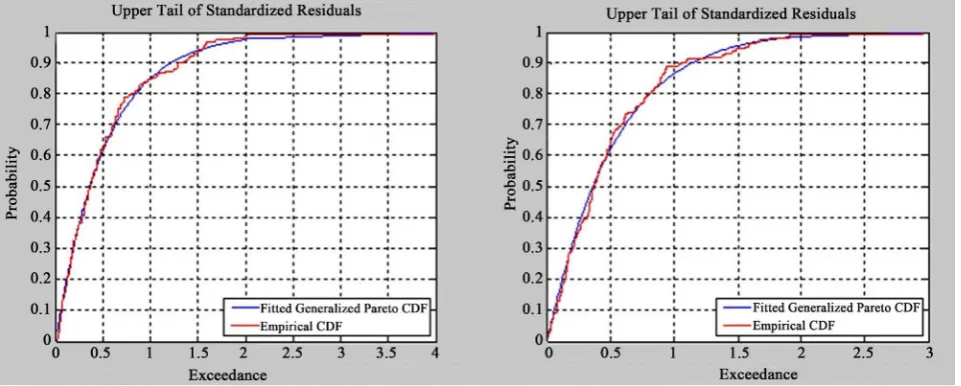
[image:10.595.207.540.460.527.2]

In the evaluation of marginal distribution, the SV-t model was evaluated first in order to obtain the standard residual sequence on the basis of the evaluated pa-rameters. Next, the tail data of the standard residual by GDP of the EVT were matched with the results presented in Table 2.

Table 1. Descriptive statistics for Hushen 300 index and HIS.

Index Average Standard _{deviation Skewness Kurtosis} J-B Q (20) Q2 _{(20) ADF}

Hushen 300

Index 0.0239 0.8715 −0.3270 5.3630 429.0*** 32.86*** 458.3*** −40.51*** HSI 0.0091 0.0339 −0.0520 11.50 5157*** 29.11*** 2093*** −42.85***

Notes: ***indicates statistical significance at the 1% level.

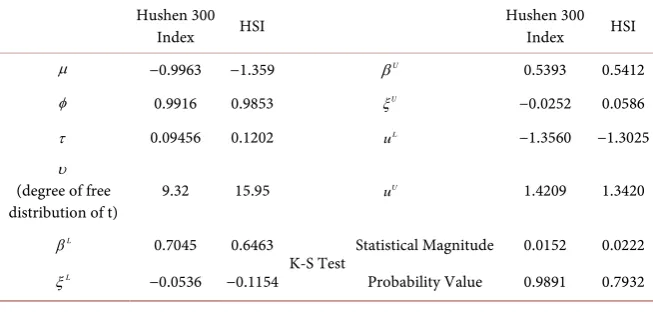
Table 2. The evaluated results of marginal distribution. Hushen 300

Index HSI Hushen 300 Index HSI

µ _{−0.9963 −1.359} βU

0.5393 0.5412

φ _{0.9916 0.9853} ξU −0.0252 0.0586

τ 0.09456 0.1202 L

u −1.3560 −1.3025

υ (degree of free

distribution of t) 9.32 15.95

U

u 1.4209 1.3420

L

β 0.7045 0.6463

K-S Test Statistical Magnitude 0.0152 0.0222

L

[image:10.595.211.538.573.729.2]

DOI: 10.4236/tel.2017.77151 2223 Theoretical Economics Letters

As is shown by Table 2, µ indicates the fluctuation range of the index for each of the two markets. In terms of absolute value, the HK index is a little high-er than that of the Chinese stock market. The φ values for the two markets are close to 1, indicating a strong continuity of fluctuation of these two markets, even though the association with the Chinese stock market is much stronger. The solution parameter τ of the model reflects the fluctuation noise for the two markets. On the other hand, υ shows that the profit rate of the two mar-kets does not follow normal distribution, as it exhibits both a remarkable peak and a thick tail. These characteristics are much more prominent in the HK stocks relative to the Chinese stock market. The tail parameter estimation of the EVT model indicates that the lower tail shape parameter of the Chinese stock market is relative to that of the HK stock market, with the number of −0.0536 and −0.1154 respectively. And the lower tail of the Chinese stock market is thicker. The upper shape parameters ξ of the two markets are −0.0252 and 0.0586, re-spectively, with the upper tail of the HK stock market being thicker. In addition, according to the concomitant probability of K-S given in Table 2, the new se-quences transformed by probability integral into the original sese-quences comply with even distribution in the [0, 1] range. Moreover, autocorrelation test of these sequences also indicates that the new sequences do not exhibit autocorrelation and are independent. The K-S test and autocorrelation test indicate that the SV-t-EVT model can describe the marginal distribution of Hushen 300 Index and HSI. In order to verify the evaluation of the tail, Figure 1 shows the GPD distribution matching effect of the upper tail overflow data of Hushen 300 index (left) and HSI (right). Hence, the model of marginal distribution based on SV-T-EVT is justified.

4.3. Evaluation of Time-Varying Copula Function

[image:11.595.60.541.512.705.2]

On the basis of marginal distribution evaluation, in this work, we apply the

DOI: 10.4236/tel.2017.77151 2224 Theoretical Economics Letters

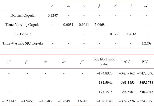
time-varying SJC-Copula model and evaluation method to analyze the correla-tion of risks associated with the Hushen 300 Index and HIS. In order to show the dynamics of time-varying SJC-Copula model and conduct a comparative study, we also conduct evaluation of this Copula model of the constant normal correla-tion, time-varying normal Copula model as well as the constant correlation of SJC-Copula model, as shown in Table 3.

[image:12.595.210.538.461.687.2]

As is shown in Table 3, there exists a proportionate correlation between Hu-shen 300 Index and the tail of HSI. More specifically, the tail correlation of nor-mal Copula is 0.4287, which is markedly different from the linear correlation of the tail at 0.4520. By using the standard residual sequence of two stock markets, the latter can be obtained with a yield of 5.4%, which is the difference between the preconditions of the normal distribution. In measuring the tail correlation of constant correlation of SJC-Copula, the correlation of the upper tail is 0.1725 and that of the lower tail is 0.2842, indicating that the tail correlation of the bear market is higher than that of the bull market. In addition, whether adopting the maximum likelihood value or sequencing by matching quality of AIC or BIC as a criterion, the time-varying normal Copula and the time-varying SJC-Copula outperform the corresponding normal Copula in the process of simulating the tail correlation. This finding indicates that the dynamic Copula is better suited for describing the correlation among variables. Furthermore, according to the minimum principle of AIC and BIC, the time-varying SJC-Copula performs better in matching the tail correlation of the two stock markets. Consequently, it can be concluded that the measuring of the tail correlation of the two stock markets by time-varying SJC-Copula is effective.

Table 3. Related copula model parameter estimation results.

δ ω α β τU τL ωU

Normal Copula 0.4287 - - - -

Time-Varying Copula - 0.0051 0.1041 2.0468 - - -

SJC Copula - - - - 0.1725 0.2842 -

Time-Varying SJC Copula - - - 2.2202

U

α βU ωL αL βL Log likelihood

value AIC BIC

- - - −173.8973 −347.7862 −347.7830

- - - −182.5944 −365.1853 −365.1758

- - - −173.1515 −346.3007 −346.2943

−12.1143 −4.9450 −1.5583 −1.7649 3.6743 −187.1148 −374.2226 −374.2036

DOI: 10.4236/tel.2017.77151 2225 Theoretical Economics Letters

4.4. Further Analysis of the Results

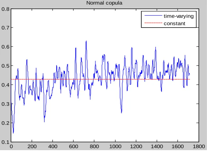
[image:13.595.209.540.464.708.2]

In order to further reveal the dynamic correlation of the Chinese and HK stock market, Figure 2 and Figure 3 show the variation tendency of time-varying correla-tion parameters of normal Copula and SJC-Copula, respectively. Figure 2 presents the constant and time-varying correlation parameters of Chinese and HK shares which obtained by the normal copula function. The tail of China stock and that of HK stock are proportionately correlated to each other, but the intensity of cor-relation is stronger than fluctuation. In terms of investment portfolio, a suitable combination of weakly correlated assets can decrease the investment risk. The static correlation analysis of the profit rates associated with Chinese and HK stocks in-dicates that a combination of these stocks can decrease the investment risk effec-tively. In Figure 2, the time-varying correlation parameter of dynamic copula ranges from 0.1438 to 0.6314. For a wide range of related parameters, the total value of dynamic copula of the time-varying correlation parameter can be great-er than or less than the constant, and the maximum value is 0.6314. Furthgreat-ermore, as is shown in the graph, the correlation of the two markets tends to increase with time.

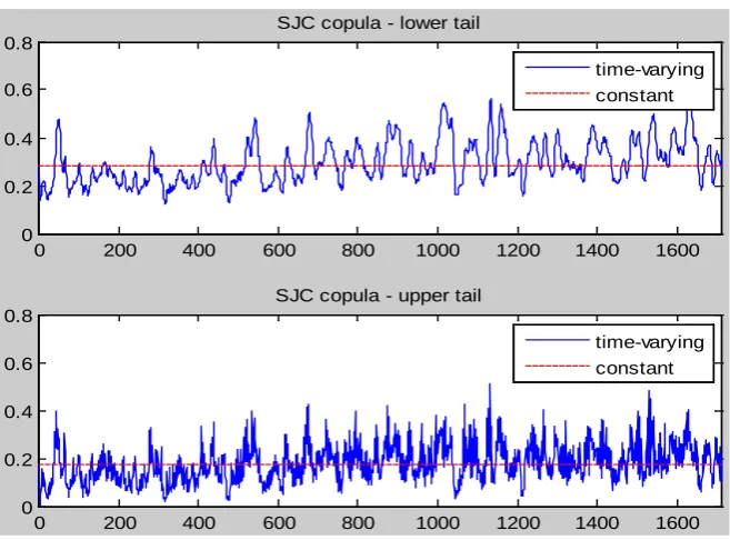
Figure 3 depicts constant and time-varying tail correlation parameters of Chinese and HK stocks provided by SJC-Copula function. The contrast of the two graphs in Figure 3 indicates that the correlation of the lower tail of the two stock markets is stronger than that of the upper tail, with obvious asymmetry. In the upper tail, the correlation fluctuates around 0.1825 and remains relatively stable during the process of opening-up China’s capital market. Absence of up-ward trend indicates low likelihood of dramatic simultaneous increases in the two market indices. In terms of the lower tail, when both markets are bear, the

Figure 2. The correlation tendency of normal copula.

0 200 400 600 800 1000 1200 1400 1600 1800 0.1

0.2 0.3 0.4 0.5 0.6 0.7 0.8

Normal copula

[image:14.595.209.538.67.310.2]

DOI: 10.4236/tel.2017.77151 2226 Theoretical Economics Letters

Figure 3. The correlation tendency of SJC-copula.

correlation parameter is about 0.3, which indicates their stronger mutual influ-ence. After the exchange rate revolution in 2005 and the issue of QDII in 2006, the tail correlation of the two markets experienced a significant increase. In ad-dition, during the process of opening-up, the time-variation of the tail correla-tion of the two markets is obvious with a maximum value of 0.5786. This is a per-suasive argument for the competence of SJC-Copula in grasping the dynamic cor-relation of the Chinese and HK stocks. This is similar to the results yielded by the comparison of extreme likelihood values, AIC and BIC, which clearly demonstrates that, when the value of one market declines, the investors pay more attention to the other market and have a great tendency to follow up. Moreover, with the ac-celerating pace of China’s opening-up to the external investment, the correlation of risks associated with the two markets becomes stronger, making both markets are more likely to suffer sudden shocks simultaneously.

Generally speaking, whether constant correlation or the time-varying copula is used, the SJC-Copula with a consideration of tail correlation outperforms the normal Copula, which indicates that the correlation between China and HK stocks exhibits an obvious asymmetry. This asymmetry can be explained from the pers-pective of investors, who would be more sensitive to news signifying low profit rather than to positive news. When the stock value begins to decline, investors become very anxious and would immediately take action; on the contrary, when stock market prices are increasing, most investors will take no action.

5. Conclusions

The correlation structure of financial assets is an important element in the anal-ysis of the financial market risks. The analyses of risks that were performed to date tended to focus on the distribution of profits of financial assets, while neglecting

0 200 400 600 800 1000 1200 1400 1600 0

0.2 0.4 0.6 0.8

SJC copula - lower tail

time-varying constant

0 200 400 600 800 1000 1200 1400 1600 0

0.2 0.4 0.6 0.8

SJC copula - upper tail

DOI: 10.4236/tel.2017.77151 2227 Theoretical Economics Letters

the different roles of the risks associated with the market as a whole and those pertaining to the individual shares. In recent years, the correlative structure of assets has started to attract much greater attention. In this paper, we discussed the correlation pattern of the financial market on the basis of time-varying co-pula. More specifically, we combined the random fluctuation model with EVT to create a new SV-t-EVT model to simulate the actual characteristics of profit se-quences of marginal distribution. On this basis, four copula models were con-structed to study the correlation between Chinese and HK stocks. As was shown in this work, SJC-Copula outperforms the normal Copula, while the dynamic Co-pula is better than the stationary one. In addition, the findings confirmed pres-ence of asymmetry in the correlation variation of Chinese and HK stocks, with the lower tail correlation much higher than that of the upper tail. As the effect of bear market is obvious, the Gaussian correlation structure in the traditional sense cannot fully reflect the correlation of the financial assets, in particular the tail cor-relation.

It is also noteworthy that, in terms of investment portfolio, risk management and assets pricing, the depiction of the correlation of financial assets, and the tail correlation structure in particular, is of great significance. Authors of extant stu-dies on the financial market correlation mainly focused on the linearity and the symmetry, rather than the correlation structure of non-linearity, asymmetry and productivity and its range of correlation. As an analytical correlation and mul-ti-statistics tool, the copula model is suitable for correlation studies, especially for financial time sequences. The dynamic Copula model can often outperform the static Copula model in depicting the correlation structure of the financial capital and financial market. However, empirical studies of dynamic Copula model are inadequate, as without the knowledge of the change of correlation, it may mis-judge the correlation structure by choosing a wrong model to simulate. There-fore, a priori estimation of the form of the correlation structure is conducive to choosing a suitable copula function. In conclusion, a new dynamic Copula mod-el is established to describe the rmod-elated structures, i.e., considering the diversified time-varying Copula and the time-variation of the degrees of freedom. While this study did not consider about the interference of the changeable regulations on the market performance in the Chinese stock market after 2013, we will ex-tend the research with consideration of the distinct regulations which highly in-fluenced in the emerging stock market to better study the topic in the future.

References

[1] Embrechts, P., McNeil, A. and Strausmann, D. (2002) Correlation and Dependence in Risk Management: Proper Ties and Pitfalls. Cambridge University Press, Cam-bridge, 176-233.

[2] Embrechts, P., McNeil, A. and Straumann, D. (1999) Correlation: Pitfalls and alter-natives. Risk, 12, 69-71.

DOI: 10.4236/tel.2017.77151 2228 Theoretical Economics Letters Opérationnelle, Crédit Lyonnais, Lyon.

[4] Zhang, T.R. (2002) Copula and Financial Risk Analysis. Statistical Research, 4, 48-51. (In Chinese)

[5] Rodriguez, J.C. (2007) Measuring Financial Contagion: A Copula Approach. Jour-nal of Empirical Finance, 14, 401-423. https://doi.org/10.1016/j.jempfin.2006.07.002 [6] Embrechts, P., Hoeing, A. and Juri, A. (2003) Using Copula to Bound the Value-at-Risk

for Function of Dependent Risks. Finance and Stochastics, 7, 145-167. https://doi.org/10.1007/s007800200085

[7] Wang, Y.Q. and Liu, S.W. (2011) Financial Market Openness and Risk Contagion: A Time-Varying Copula Approach. Systems Engineering-Theory & Practice, 4, 778-784. [8] Patton Andrew, J. (2006) Modeling Asymmetric Exchange Rate Dependence.

In-ternational Economic Review, 2, 527-555.

[9] Gong, P. and Huang, R.B. (2008) Analysis of the Time-Varying Dependence of For-eign Exchange Assets. Systems Engineering-Theory & Practice, 8, 26-38.

[10] Li, X.M. and Shi, D.J. (2006) Research on Dependence Structure between Shanghai and Shenzhen Stock Markets. Application of Statistics and Management, 25, 729-736. (In Chinese)

[11] Ren, X.L., Ye, M.Q. and Zhang, S.Y. (2009) Analysis of Portfolio Efficient Frontier Based on Copula-APD-GARCH Model. Chinese Journal of Management, 6, 1528-1535. (In Chinese)

[12] Yu, S.H., Zhang, S.Y. and Song, J. (2004) Comparison of VaR Based on GARCH and SV Models. Journal of Management Sciences in China, 7, 61-65. (In Chinese) [13] Bollerslev, T. (2001) Financial Econometrics: Past Developments and Future

Chal-lenges. Journal of Econometrics, 100, 41-51. https://doi.org/10.1016/S0304-4076(00)00052-X

[14] Zhan, X.L. and Zhang, S.Y. (2007) Risk Analysis of Financial Portfolio Based on Copula-SV Model. Journal of Systems & Management, 3, 302-306. (In Chinese) [15] Ramazan, G. and Faruk, S. (2006) Overnight Borrowing, Interest Rates and Extreme

Value Theory. European Economic Review, 50, 547-563. https://doi.org/10.1016/j.euroecorev.2004.10.010

[16] Zhou, X.H. and Zhang, Y. (2008) New Calculation Method and Application of Val-ue-at-Risk (VaR). Chinese Journal of Management, 5, 819-823. (In Chinese) [17] Wei, Y. (2008) EVT Risk Measures and Its Back Testing in Stock Markets. Journal

of Management Sciences in China, 11, 78-88. (In Chinese)

[18] Cherubini, U., Luciano, E. and Vecchiato, W. (2004) Copula Methods in Finance. John Wiley & Sons Press,Hoboken, 37-95. https://doi.org/10.1002/9781118673331 [19] Bouyé, E., Durrleman, V., Nikeghbali, A., Riboulet, G. and Roncalli, T. (2009)

Co-pulas for Finance—A Reading Guide and Some Applications.

https://ssrn.com/abstract=1032533

[20] Durrleman, V., Nikeghbali, A. and Roncalli, T. (2009) Copulas Approximation and New Families. https://ssrn.com/abstract=1032547

[21] Embrechts, P., Kluppelburg, C. and Mikosch, T. (2008) Modeling External Events for Insurance and Finance. Springer, New York.

[22] Bhatti, M.I., A1-Shanfari, H. and Hossain, M.Z. (2006) Econometrics Analysis of Model Testing and Model Selection. Ashgate Publishing, Farnham.

DOI: 10.4236/tel.2017.77151 2229 Theoretical Economics Letters https://doi.org/10.1111/1467-937X.00050

[24] Ramazan, G. and Faruk, S. (2004) Extreme Value Theory and Value-at-Risk: Rela-tive Performance in Emerging Markets. International Journal of Forecasting, 20, 287-303.https://doi.org/10.1016/j.ijforecast.2003.09.005

[25] Dempster, M.A.H. (2002) Risk Management: Value at Risk and Beyond. Cambridge University Press, Cambridge, 176-223.https://doi.org/10.1017/CBO9780511615337 [26] Lin, Z.J. and Tian, Z. (2012) Accounting Conservatism and IPO Underpricing: