Some studies in optimum and self adaptive control systems

University of Warwick institutional repository: http://go.warwick.ac.uk/wrap A Thesis Submitted for the Degree of PhD at the University of Warwick

http://go.warwick.ac.uk/wrap/61752

This thesis is made available online and is protected by original copyright. Please scroll down to view the document itself.

by

K.K. Murthy.

B.E •• M.E.

A thesis submitted to the University

of Warwick for the degree of

Doctor of Philosophy

School of Engineering Science

AVAILABLE

Acknowledgements (i)

Preface (ii)

PART I - Performance of the Second-order

Relay Servo under Non-ideal

Operating Conditions. 1

List of Principal Symbols. 2

l~ Introduction.

2. The Optimum System.

2.1, The Total Response Time.

3.

Effect of Departures from Ideal

Switching Conditions.

3.1.

Errors in the Switching Locus.

3.2. Effect of Friction.

3.3.

Relay Hysteresis and Threshold.

3.4. Time Lags and Time Delays.

4. Sensitivity of the Optimal System.

5. Stability of the System.

6. Analogue Computer Studies.

6.1 •. Discussion of Results.

7.

Conclusions.

8.

Appendices.

A~l. Derivation of Response Time when

4

10

15

16 16 17 19 19 20 26

33

35

37

,

A.2.

wp>wo'

Derivation of Response Time when

wp<wo'

The Published Paper.

38

A.3.

40

44

PART II - Self-Optimisation using

Pseudo-Random Binary Sequences. 45

List of Principal Symbols.

47

1. Introduction. 50

3.2. Response of a Particular System. 69

4.

System with .Continuous Parameter Adjustment. 73 4.1. Response of a Particular System. 80

4.2. Dynamic Compensation. 81

4.2.1. Experimental Results. 82

5.

Effect of Noise. 5.1. General.

5.2. Evaluation of Variance.

85

86 5.2.1. Variance of System with

Discontinuous Adjustment. 86 5.2.2. Variance of System with

Continuous Adjustment.

89

5.3.

System Response in the Presence of Noise.

6~ Stability of the System with Continuous Adjustment.

92

6.1.

6.2.

6.3.

General.

System without Dynamics. System with Dynamics.

93

96

99

7.

The Electro-Mechanical Running Averager.

7~1~ General. 103

7.2.

Methods of Simulation. 105

7.3. Principle of Operation. 106

7.4.

Construction of the Running Averager. 109

7.5.

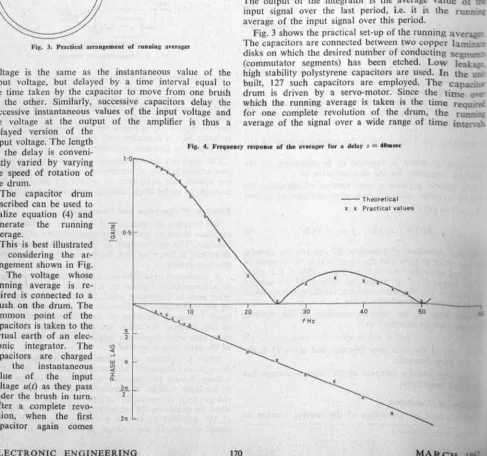
Frequency Response of the Running

Averager. 111

8~ Special Computing Elements. 112

9.

Methods of Synthesis of New Binary Sequences.

9.1. General. 115

9.2. Method of Synthesis using a

Non-Linearity. 115

9.3. Method of Synthesis using Impulse

Trains. 121

9.3.1. Necessary Conditions for the

New Sequences. ₁₂₈

131 10. Conclusions.

11. Appendices.

A.1. Properties of Pseudo-Random

Binary Sequences. 134

A.2. Gain of Adaptive Loop. 137

A.3. Relationship between the Starting

Point of the Chain Code and the

Transient Factor a. 140

A.4. Calculation of the Theor~tical

Response for the System with

Continuous Parameter Adjustment~ 141

A.5. Proof that Certain Types of

Auto-Correlation Functions are

Unrealisable. 147

A.6.. The Published Papers. 148

PART III - Frequency Re9~onse of Linear

Sampled-Data ystems.

1. 2.

3.

4.

Introduction.

Derivation of Gsb(jw)

Stability AnalysYs. Conclusions.

149

150

152

155 158

ACKNOWLEDGEMENTS

The author wishes to acknowledge with gratitude

the continual guidance and encouragement of

Professor J.L. Douce and Dr. K.C. Ng and expresses

his appreciation of the many helpful discussions

with his colleagues. during the course of the work

described in this thesis. The author is also

grateful to the Commonwealth Scholarship Commission

in the United Kingdom for the Scholarship award

and to the Board of Governors o~ the Regional

Engineering College. Durgapur. for the grant of

PREFACE

This thesis presents the results of a three

year research project carried out by the author

from October. 1964 to June. 1967 while a

Commonwealth Scholar in this country.

The contents of the thesis are divided into

three parts.

Part I describes the analytical and experimental

studies on a seoond-order b~ng-bang ~ervo under

non-ideal operating'oonditions.

The sen~itivity and

stability of the bang-bang system have been,

investigated •., This work

.waa

oarried' out during

1964-65 while a,researoh scholar at the Queen's

Univer~ityof

Belfast,

Part II of the thesis is entitled "Self-optimisation

using Pseudo-Random

Binary Sequences".,

In this part.

the performance of the original hill-climbing

system

which employs discontinuous

parameter adjustment and

of the modified system using continuous paramet~r

adjustment is described.

It is shown that the system

with oontinuous parameter adjustment has a superior

performance.

A novel analogue running averager has

Part III describes an invest~gation

into the

frequency response of a sample-and-hold

element at

certain sampling frequencies.

As a result of the work described.

three papers

have been published and a fourth one has been

accepted for publication.

1.' "A Note on the Performance

of the Second-order

Maximum Effort Controller", X.K. Murthy.

International

Journal of Control, Vol.2, No.3.

September,

1965.

2.' "An Electro-Mechanical

Running Averager",

K.C. Ng and K.K. Murthy. Electronic

Engineering.

March, 1967.

3.

"Recent Advances in a Hill-climbing

System",

X.C. Ng, K.K. Murthy, D.H. Stockwell and

K.R. Morris, Second I.E.E. Convention

on

Advances

in Computer Control, Bristol,

April, 1967.

(Paper 1 is based on Part I and papers 2 and

3

are based on part II)

4.

"Frequency Response

of Linear Sampled-Data

Control Systems", J.L. Douce, X.C. Ng

accepted for publication in 'Controlto

(This paper is based on part III)

All the published papers are enclosed in the

PAR T I

PERFORMANCE OF THE SECOND-ORDER RELAY

SERVO UNDER NON-IDEAL OPERATING

CONDITIONS

SUMMARY

The behaviour of a second-order bang-bang

control system when the system parameters are varied

is investigated. For non-ideal operating conditions.

the response of the bang-bang servo is compared

with that of a saturating servoo The sensitivity

of the bang-ban.g servo for variations in the system

dynamics has been examined. The stability of the

system in the presence of additional time delays

and time lags is investigated. Analogue computer

LIST OF PRINCIPAL

SYMBOLS

9

i

::: Input position and input signal.

90 :::

Output position and output signal.

::: :::

=

_{Error signal.}

:::

:::y

=

Output velocity.

u,~

=

Control signal.

a

:::Maximum

developed

torque.

1 .

=

¥

:::

Undamped

resonance frequency.

:::Motor field build-up time constant.

TD

=

Delay time.

TR

=

Response time.

TAB

::: Time taken to travel over the phase path AB.

Kv

=

Gain factor of the stabiliser.

:::

Gain factor of the error processing

non-linearity.

S

=

Switching function.

:::

Initial position x(o).

:::

Coefficient

of viscous friction damping.

w = Plant parameter vector.

:: Nominal design value of motor acceleration.

= Actual motor acceleration.

= Relative sensitivity.

= Maximum value of relative sensitivity.

G(p)

N(m)

= Transfer function of the process.

:: Describing function.

= Phase angle of describing function.

R :: Magnitude of describing function.

1. INTRODUCTION

There are essentially two approaches to the

optimal control problem. One is concerned with

optimising the responses of the controlled variable

to disturbances of the system to be controlled. For

a single variable system. at each instant there is a

known desired value of the controlled variable. The

control engineer is primarily concerned with keeping

the maximum error to a minimum. and then with such

other aspects of the response as the number of

oscillations in the transients due to step disturbances,

the magnitudes of overshoots and undershoots, and

their durations. He is interested in the entire

response and thus simultaneously in many indexes of

performance. Reduction of the maximum system error

cannot normally be achieved regardless of the magnitude

of a step change. over the reduction tha~ can be

attained with linear control functions. Tests have

shown that simple non-linear control functions

definitely improve system response.

The early control engineers intuitively assumed

that any control system error which did not demand

if the maximum available control effort were applied.

Thus, when the control signal is constrained to take

on only its maximum or minimum values. it is called

a 'Steering Function'. Minimum response time is

obtained only if the sign of the steering function

is caused to change in the proper manner.

A 'Switching Function' is the function of the

controlled variable and its derivatives that defines

all the instants at which the steering or control

function must change sign for minimum response time.

A lot of work has been done on these optimum

switched systems. Minimum response time control was

obtained for an Aircraft engine propeller system as

early as 1944 by Oldenbergerl• In 1950, Mcdonald2

published a paper on th~ on-off time optimal control

of second-order systems with bounded inputs. This

was followed in 1951 by phase plane, topological and

analogue computer studies of the same system by

Hopkin

3,

Uttley and Hammond4• Flugg-Lotz5

..

published

a book in 1951 on the bang-bang control of

second-order systems with linear switching functions. West

et a16 in 1954 proposed a method of mechanising the

The second approach to the optimal control

problem is essentially a mathematical one. Busha~4

in 1953. originated this approach. In 1956. Bellman

et al9 gave a general treatment of the optimal

problem. In 1957. the Russian mathematician

Pontryagin published his maximum principle explained

in 1959 by RosonoerlO. Lasalle11 proved that an

on-off control system is the time optimal systemo Since

then. various authors have reported further work on

the mathematics of optimal systems.

In the work being reported in this thesis, the

first essentially engineering approach is takeno

The simplest example of a bang-bang servo is the

relay actuated servo motor position controllero In

all relay or bang-bang control systems, the system

always operates under maximum actuating torque

conditions. For half the time, maximum accelerating

torque is developed and for the other half maximum

e

de~leration torque is developed. In other words.

the direction of the torque is reyersed at exactly

second and fourth quadrants passing through the

origin. The switching from acceleration to

decele-ration takes place on this parabolic switching curveo

Such an optimum switching can be achieved by a suitably

designed non-linear e.rror processing deYice6 to actuate

the relay.

The operaticn of such a switched relay servo

system has been obtained under the following

assumptions:

(i) Inputs limited to step functions.

(ii) Instantaneous switching on the change-over

boundary.

(iii)

(iv)

No time delays present in the syst&m.

Accurate knowledge of the motor dynamics.

The limitation on the admissible inputs is in

general. severeo Bushawl2 has shown that f'or the

response to be optimal. only steps and ramps are

admissible as inputs to the pure inertia servo and

only steps are admissible inputs for the servo with

inertia plus Coulomb or viscous friction.

response and shown that considerable improvement in

performance can be achieved for sinusoidal inputs

also. '

The other two assumptions tend to be in general.

idealistico In practice. instantaneous switching on

the reversal curve cannot take place and finite time

delays have to be taken into account. In addition,

relay r~steresis, contact spacing, etcoo tend to

deteriorate the performance of the system., Time

delays have the effect of permitting the state of

the system to over-travel the switching trajectory,

reverse, over-tr~vel again and so forth. Thus the

trajectory may approach a terminal limit cycleo The

effect of inputs other than the ones considered in

the initial system concept. can also have disturbing

consequenceso

These remarks emphasize the fact that the on-off

control system can be extremely sensitive to variations

in system parameters. The qualitative nature of the

deterioration in performance under the non-ideal

conditions is investigated in this work. It is compared

with the performance of a saturating servo system

with a small linear regime and shown that the

additional lago The sensitivity of the system for

variations in the motor dynamics is examinedo If

the range of variations of the system parameter is

known, it is shown that by suitably designing the

switching curve, the response can be made to be least

2., THE OPTTMUM SYSTEM

The system used for the analysis is schematically

shown in Fi.g"lo The torque limited servo motor is

actuated by a relay so that the motor always develops

maximum torque the direction of which depends upon

the position of the relay or the sign of the control

signal uo Frictional forces in the motor are neglected.

The transfer function can then be represented by

G(p)

Th.e Equations of the switching curves or traj

ee·t-ories on which the po Lar-Lty of the control signal is

reversed is to be derivedQ since these are necessary

for synthesisi.ng the controller. Either a differential

equation approach or a matrix notation can be used.

The matrix notation is particularly suitable for

higher order systems.

For the system under consideration.

to

(1)

90 = ul • • •• 0

By defining

XJ.

= 90

•

x2 =

the system Equation can be written in the matrix form

e x

-

A x + Bu o 0 • • 0 (2)

where

A is an n x n matrix9 B is an n x m matrix

(m ~ n )9 .! is an n-vector and u an m-veot or-,

In our caseQ

The solution of Equation (2) is obtained by the

method of variation of parametersQ and is given by

Bellman9 as

x

=

-1

Q

B u dt ₊ 00000 (3)

where the matrix

Q

is defined in such a way as to

satisfy the Equation

o

Q = 'A Q • • • • 0

and Q(O) = I • • • • 0 (5 )

and ~o is x at t = 00 (~o lies on the last

Equation

(4)

represents four simultaneous differential

equations:

o o o •

(6)

The solution of this set of equations with the

constraints of Equation (5) yields

• • • •• (7)

••••• (8)

When t = T, origin is reached and from Equation (3)

we get

T

- f

o

Solving the two simultaneous equations represented

x =

-0

-1

-Q B u dt ••••• (9)

by _{(9) •} we get

u T2

Xo =

_-r

1 9 Xo = - u1T

1 2

Eliminating T between these two Equations, the

s

=

x 2

2

2ul =

o

••••• (10)

Equation (10) defines the curve in the phase plane

at which the control function ~ must change sign

for optimal response. On the phase plane (Xl=X,

x2=y), Equation (10) becomes

s

= _{x -}

o

••••• (11)

which is the Equation of a Parabola.

For the system of Figol,

= = +_{- --2}a

T

where 'a' is the maximum torque developed by the motor.

Hence Equation (11) can be written as

s

= +

_~

2ax

₌

T

o

•• ••• (12)

positive sign in Region (i) and negative sign in

Region (ii).

s

₌ y _{Iyl +} 2ax 0 (13)

7

= •• • ••

for S< o , the output of the relay is positive

for S >0. the output of the relay is negative

In Fig.2. ABC is a typical trajectory. With

correct reversal from acceleration to deceleration

on the critical trajectory, the response will be

optimumo This means that for minimum time of response.

all the constant acceleration trajectories from

different initial conditions must change over to the

same critical decelerating trajectory through the

origino

At the point of change-over B.

= - h /2

o

1/2 (aho/T')

)

l

• • • •• (14)

=

The optimum change-over can be achieved by

mechanising Equation (13) using a non-linear error

processing device and a linear velocity feedback

stabilisation ter.m which has been called the SERME

2.1. The Total Response Time

The total time of response can be calculated easily

from the above equations.

It is assumed that no over-shoot is to occur at

c.

in Region

(i)

Integrating,

.

_at/T2

eo =

At B, 90

.

=

_YB = atIlT2

Hence _TAB = _YBT2/a

Substituting for YB from Equation (14), we get

=

Since the change-over takes place at the half-way point

=

••••• (15)

Thus from Equation

(15),

it is seen that the response

time is dependent on the magnitude of the input step

only since 'a', th~ maximum torque developed is a

constant for a given servo motor. The response time

versus the input step magnitude characteristic is

,

30 EFFECT OF DEPARTURES FROM IDEAL SWITCHING

CONDITIONS

It is again emphasised that the response of the

system is optimal only when the assumptions of Section 1

(page

7)

are valido In this Sectionv some of the

common practical departures from the ideal conditions

and their effect on the system response are consideredu

3010 Errors in the Switching Locus

When the switching trajectory is mechanisedv the

actual realisation of the switching curve may not

follow the ideal parabolic curve exactlyo Let us

first consider the effect when the actual switching

curve is nearer to the error axis than the ideal

curveo This is shown in Figo3(a)o Ar~ representative

point P moves along the acceleration trajectory till

it meets the change~over boundary at PI at which the

relay re~e~es the torqueo The system must then

follow a deceleration trajectory. The switching

locus itself is not a deceleration trajectory, so the

state point tries to follow the deceleration trajectory

.

"

P P which passes through Plo This causes the relay

to reverse again and follow an acceleration ~rajectory

switching locus to the origin with the relay

chatter-ing at high frequency. This response of the system

is slower than the ideal response.

On the other hand, if the actual switching

trajectory is nearer to the y-axis than the ideal,

the motion is shown in Fig.3(b). Relay reverses at

PI' follows the deceleration trajectory through PI'

reverses again at P2 and so ono Thus, the system

has overshoots and undershoots and the amplitude of

successlve oscillations decreases and the frequency

increases until the system reaches the origin.

3020 Effect of Friction

The effect of friction on the ideal trajectory

has been studied by Kazdal59 Stoutl6, Flugge-lotz

5

and otherso In principle, the presence of Coulomb

friction results in bringing the error rate to zero

but not the error when the steady state is reached.

This is not true in practice. In the presence of

friction. in practice, end-point oscillations (a kind

of convergent hunting) as shown in Fig.4(a) are

observed. This results in a larger time to reach the

steady state. If the magnitude of the Coulomb

switching from acceleration to deceleration, improved

performance can be obtained. With this modification

the Equation of the switching trajectory in the

fourth quadrant becomes

s

= 2a (1 + aC) x

T2

a

instead of Equation (12) where ac is the magnitude of

Coulomb friction torqueo

If the effect of viscous friction has to be taken

into account properlY9 new switching trajectories

must be derived by solving the Equation

+ =

instead of solving Equation (1).

The solution of this yields the Equation of the

switching trajectory

s

= = 0

It is seen that the Equation of the switching

3.3.

Relay Hysteresis and Threshold

The presence of Hysteresis and Threshold in the

relay characteristic delays the change-over from

acceleration to deceleration. The delayed trajectories

are shown in Fig.4(a). The delayed trajectories are

also parabo1ico Because of the delayed trajectory

not passing through the origin. terminal limit cycles

are observed

17•

These limit cycle oscillations can

be stable or unstable. The system thus performs

wasteful gyrations resulting in an increase in response

time~ •

3.4.

Time Lags and Time Delays

Time delays and time lags are inevitably present

in any practical system. The effect is again to delay

the change-over from acceleration to deceleration.

The effect of time delay is shown in Fig.4(b). These

may produce terminal limit cycles. If the time constant

of the lag and the delay times are known. the magnitude

and frequency of the limit cycle can be calculated

40

SENSITIVITY

OF THE OPTIMAL

SYSTEM

In any successful optimal design. the achievement

of the desired response and its relative insensitivity

to system parameter changes or for small component

imperfeotions is one of the basic requirements. In

many applicationsQ the invariability of the response

or the insensitivity to parameter changes is even

more im.portant than nominal behaviour.

Consider the general control process described

by the Equation

•

x

=

f [

~(t).~(t).~ ]

.0000

(16)

where

~ is the state vector

~(t) is the control vector

w

is the plant parameter vector

If

C =

T

f

¢(x,u..) dt

o

--••••• (17)

is the performance index on the basis of which the

optimum ~ is determined, then by solving Equations

Let

U opt =

t [~(

t ).

z,(

t). t ] ••••• (18)

The plant parameter vector ~ which appears in

Equation (16) seldom corresponds to the value of ~

in Equation (18) due to component inaccuracies,

environment effects, etc. Hence if w is the actual

-p

value of the plant vector, then from Equations (16)

and (18), we have

i

=

f [ ~(t). {~[ ~(t). :!!o(t). t

J}

'!!pJ

Optimum operation requires that ~o

=

~p'

For every actual plant parameter value ~p' a best

value of ~o exists such that the performance index C

has an optimum value. Under such conditions, when

W is varying, C can be considered as a function of

-p

~o and wp' Therefore variations in C due to small

parameter variations is given by

AC

=

Analytical solution for the evaluation of

AC

is in

One possible criterion of performance based on

the insensitivity to parameter changes would be to

minimise the maximum deviation from the optimal

behaviouro This can be achieved by evaluating the

"Relative sensitivity" and choosing the control

parameter such that the maximum value of the relative

sensitivity is a minimum19•

Relatiye sensit.ivity for the control ~(t) is

defined19 to be the difference between the actual

value of the performance index C(!!oowp) and that

which would be obtained if the control were the

optimal for the plant paramet ez- w 9 C(w ,wp> divided

.. -p p

-by the optimal performance index for normalisationo

=

c

(!!o9!_P) C(!!p'!!p)

I

C(!!pII

.!p )

I

••••• (19)

It is seen from Equation (19) that the relative

sensitivity SR is always a positive number and that

the optimal value of SR is zero. regardless of the

value of the performance index itself.

The relative sensitivity function can now be

evaluated for the bang-bang system considered in

From Equation (1). the plant considered in Section 2

is described by

=

₌

where lui~ 1

The control signal u is given by

u ~ - sign [

xl/

2 + y

]

(2w )1/2

o

where

2

When wp

=

woQ the system is optimal.

For a given range of variation in wp(i.e. in

'a)

a suitable value of wo(ioeo

XV)

can be chosen such

that the maximum relative sensitivity is a minimum

thus resulting in a system which is relatively

insensitive to these variations.

The performance index for this system is the time

to reach the optimum from 'any initial point in the

phase planeo From Equation (15), the response time

=

₌

••••• (20)

Let us consider the normalised system in which

h =1, and nominal w =1. wTl is assumed to vary in the

o p ~

range 0.7,wp,lo3. That is a variation of ~30 percent

from the nominal value.

When wp>wo' as discussed in Section 3.1. the

system chatters to the origin along the switching

curve and the response time can be shown to be given

by (Appendix Aol)

=

•• •• • (21)

However. when wp<wo' again as discussed in

Section 301. an infini·te number of switchings are

required for the state point to reach the origin and

the response time can be derived as (Appendix A.2)

From Equations (20), (21) and (22). the relative

sensitivity

sR

is given by

[1+

. 1/2

sR

1 _~

]

1 ,

=

-12

Wo

..(2

=

_{w 1/2 w -w}

_1/2

(l+wE)

[l-(wO

+wP) ]

o 0 p

1 , W ~w

p 0 ) ) )

l

₎ ~ ~ (23) •••••

Equation (23) is plotted in Fig.5 as a function of

wp over the assumed range of wp for different values

of wo. The value of Wo is to be chosen such that

the maximum relative sensitivity SM is a minimum.

From Fig.5 it is seen that

SM (0.7, 1.3)

₌

0.2

SM (1.3. 0.7) = 1.45

8M (1. 0.7) = 0.89

and so on. Hence _Wo

₌

0.7 gives the minimum value

for SM. Thus. when Wo is chosen ~s 0.7. the response

time will be'within ~ = 2.35 seconds for a

varia-.f0.7

tion of wp in the range 0.7,Wp,1.3. Hence by choosing

.

the switching curve corresponding to wo=0.7. the best

In this Section, the stability of the relay servo

considered in Section 2 is discussed. As stated in

Section 3. presence of time delays,.lags, etc. are

inevitable in practice and their presence gives rise

to non-ideal switching trajectorieso The object of

stability analysis for the bang-bang servo is to

determine the magnitude and frequency of the limit

cycle that may be present due to the non-optimum

operating conditions that may exist.

The system of Section 2 can be represented by the

block diagram of Figo6(a)o The stability analysis of

the system of Fig06(a) is difficult since the two

non-linearities are not in simple cascade. Since the

purpose of the non-linearity NI and the velocity

feed-back signal is to satisfy Equation (13), these can

be replaced by a single non-linearity satisfying the

boundary Equation (13)0 The equivalent system is

shown in Figo6(b)o The control computer obeys

Equation (13) and generates the control signal ec•

I

Now since NI and N2 are in simple cascade, stability

analysis is possible by the describing function

•

and N2 is only amplitude dependent. The frequency

•

dependent describing function of NI can be evaluated

from Equation (13). It is assumed that the system

has sufficient low-pass filtering effect so that the

harmonics above the fundamental ma.y be neglected.

The non-linearity N2 is of zero memory type and

does not 'introduce a phase shift to the describing

•

function. But NI contributes a phase shift to the

describing function which can be evaluated (Fig.7).

Let N(m) be the describing function of the two

non-linearities in cascade. Let

N(m) = R exp (j¢) ••••• (24)

If x = m cos wt,

. ';~I~""

the output of N2 is a square wave of magnitude ~a.

Hence the magnitude R of the describing function is

R , ••••• (25)

The phase shift

¢

is calculated by considering

!

the control computer.

The control computer in Fig.6(b) evaluates the

2ax

ec

=

Y IYI

+ ~

The phase shift is found by evaluating the instant

at which ec goes through zero

(Fig.?).

Considering

the one half.cycle in which Y does not change sign,

2am

m2w2

')

ec ₌

T2 cos wt

-

san" wt

ec ₌ 0

when

2am

cos wt m2w2 sin2 wt 0 (26)

. T2

-

=

• • • • 0

Solving Equation (26) for cos wt, we get

I

cos

wt

=

cos 9

=

f.;{-

;2

+

[<;/

+

<w

2

ml

2J ~ }

The phase angle

¢

of the describing function

=

the

phase angle at which x passes through zero the

phase angle

e.

Therefore

N(m)

= ~

exp

{j

Sin-{

*{;~

+ [(;/ + (w2

m)

2J

2}]}

••••• (27)

The amplitude and phase of N(m) as a function of

m are plotted in Fig.8.

If G(jw) is the transfer function of the control

process, then by Nyquist stability criterion, the

limit cycle must adjust itself to satisfy the Equation

- N(m)

=

_G(jw)

1 • • • • •

(28)

The limit cycle may give rise to stable or

unstable oscillations.

This' can be easily checked

•

by plotting

_G(1

_jw)

and

- N(m).

Since - N(m) is

frequency dependent. a family of N(m) curves for

different values of ware

to be plotted in the G(jw)

1

plane.

The point of intersection of

G(jw)

and

- N(m)

that corresponds to the same frequency on

both the curves gives the magnitude an~ frequency of

the limit cycle.

Alternatively. an analytical

solution can be obtained by equating the amplitudes

Simple Lag

:-If a simple lag representing the motor field

build-up time constant which was neglected earlier,

is included with the process of Section 2,

where Tl is the time constant of the lag.

Hence from Equation (28)',we have

1

=

CA)2T2(1

+

w2Ti)2 exp

[j

tan-l(WT'l)]

••••• (29)

The amplitude and frequency of the limit cycle

are obtained by equating the magnitudes and phase

This results in

w

=

0..

447

T1

Tl 2

5061 a (r)

} ••••• (30)

m =

From Equation (30) the amplitude and frequency

of the limit cycle can be calculated. It is seen

that the period of the limit cycle is proportional

to TI and the amplitude proportional to (TI/T)2.

Time Delay

:-If a pure time delay of magnitude TD is present

instead of a lag of time constant TI, proceeding in

a similar way, it can be shown that

w = 00485

TD

Tn 2

m = 5042 a (r)

} ••••• (31)

Thus the period and amplitude of the l~mit cycle

are again proportional to TD and (Tn/T)2 respectively.

Time Delay and Time Lag

-:-If both the time delay and the lag are present,

the same method can be applied to derive expressions

It can be shown that

1

w2=

-(Tl+TD)(~2+8)+{~4(Tl+TD)2+16rt[Ti+(Tl+TD)2J}2

2(Tl+Tn)[~2Ti-4(Tl+Tn)2]

m

=

•• ••• (32)

From Equation (32). wand m can be evaluated

6. ANALOGUE COMPUTER STUDIES

As pointed out in Sections

3

and

4.

the bang-bang

system is sensitive to departures from ideal operating

conditions and parameter variations. The deterioration

in the performance of the ideal system under these

operating conditions is studied by simulating the

system on the analogue computer. For comparison of

the performance under these different operating

conditions, a common performance index is necessary.

The time required to bring the state point to the

origin from an initial state in the phase plane is

chosen as the performance index. The response time

(TR) is defined to be the time taken for both the

error and error rates to become zero simultaneously

following an initial step disturbance to the system.

,

In the presence of terminal limit cycles, the error

I

and error rates cannot become zero. Hence response

time is reckoned as the time required to bring the

error and error rates into a small region around the

origin. This region is chosen to be a small rhombus

enclosing the origin.

The performance of the bang-bang controller is

parameter chosen for variation is the gain factor of

the stabilising network. When the stabiliser gain

factor is adjusted to have the critical value. the

bang-bang system has the optimal response and the

state point reaches the origin without any overshoot.

It ia easily seen that the critical value of the gain

factor is given by

K (critical)

V'

where Kl is the gain factor of the error processing

non-linearity.

The effect of additional lags representing field

build-up time constant of the motor on both the

bang-bang system and the saturating system are

studied. The magnitude and frequency of the terminal

limit cycle when the additional time lag and time

delay are present are measured and compared with the

calculated values using Equation (32).

The block diagram of the analogue computer set-up

is shown in Fig.9. The non-linear unit$ are built

using biased diode circuits. The bang-bang

characte-ristic has negligible hysteresis and threshold

effects. Response time ls measured by measuring the

a constant DoCo voltage is applied at the same instant

as the input step is applied to the systemo The

time delay is simulated using fourth order Pade'

approximation58• In the simulation. the saturation

characteristic had a slope of 10 and the time constant

1

of the additional lag

-ro

the integrator time

constanto

601. Discussion of Results

The results of the computer studies are shown

in Figs. 10 and 11. It is seen that, from Fig.lO,

the theoretical and the practical response time

characteristics agree very closely for the system,

under the ideal conditions. It is seen that the

saturating system with the stabiliser gain set to

correspond to critical damping takes about 5 percent

more time to reach the origin than the bang-bang

system with critical stabiliser gain. Fig.ll shows

the response time characteristics for the different

non-ideal conditions. The bang-bang system is more

sensitive to changes in stabiliser gain than the

saturating system as can be seen from Figs.ll(a) and

ll(b). The response time increases by about 32 percent

value by 10 percent I.n the case of bang-bang system,

as compared to an increase of about 13 percent only

for the saturating system. The magnitude of the

overshoot or undershoot for the bang-bang system

can be calculated from the expression

[

K2. I)

]

ho 1 T'z,

Ta

-

··~v

x ₌

o.s ..

[ Kf

₊

_{K; ]}

2a

where ho is the magnlt:ude of the step input"

The inclusion of the additional lag introduces

terminal limit cycles.. The response time for the

bang-bang system increases by about 45 percent with

the lag as compared to an increase of onl.y 3 to 4

percent for the saturati.ng system, as can be seen

from Figs ..ll(c) and (d) ..

When both a time delay and a lag are included,

the magnitude and frequency of the resulting limit

cycle in the bang-bang system has been measured ..

Fig.12 shows that the measured values agree closely

7. CONCLUSIONS

From experimental studies on the Analogue

computer, it has been shown that the performance of

the bang-bang controller is optimum only when the

conditions obtainable are ideal. In the presence

of switching curve errors, time lags and time delays

the saturating servo has a better performance. The

bang-bang servo is more sensitive to parameter

variations and non-ideal conditions than the

saturat-ing servo. The linear operating regime in

thesatu-rating servo is also extremely useful in eliminating

terminal limit cycles.

The stability of the SERME system has been studied

and expressions for the magnitude and fre~uency of

the limit cycle have been derived. Experimental

\ vfilues agree closely with the theoretically predicted

~:

values.

When the motor dynamics vary. if the range of

these variations are known, it has been shown that

by suitably altering the switching curve it is

possible to obtain a system response which is least

8.

APPENDICES

A.1. Derivation of Response Time when w'> Wo

When the motor dynamics are such that wp>wo'

the nature of the response is similar to the case

when the switching curve is nearer the error axis

than the ideal curve as discussed in Section 3.1.

The state point reaches the origin along the

switch-ing curve, the relay chattering at high frequency.

For the calculation of response time, it can be

assumed that the system moves to the origin along

the switching curve. A typical trajectory is shown

in Fig.lJ(a) 0

•

The system Equation is given by

..

x =

The time required for the path PPI [Figo13(a)]

is given by

•••• 0 (A.1)

The motion along the path PP1 is described by

2 ;2

(xP1- ho)

Y - Yo = - 2w

P1 P

2

(xp - ho> (A.2 )

or

As point

PI

is on the deceleration trajectory

passing through the origin.

YPI

is also given

by

= ••••• (A.3)

(A.2) and

1/2 (2wpho)

wn

1/2

(1+ ~)

o

(A.3). we get From Equations

••••• (A.4)

Hence

1/2 (2ho)

• ••••

(A.5)

The response time for the path PlO is given

by

YPI

_(2W

₁₂

_ho)1/2

TPIO

=

_-

= _{W 1/2}

Wo

wo(l+

vf2)

0

The total response time is hence

1/2 W 1/2

(2ho) (1+

vr-)

o

W 1/2

p

A.2. Derivation of Response Time when w (wo

When wp<wo' the nature of response is similar to

the case when the switching curve is nearer the y-axis

than the ideal curve. There will be more than one

intersection of the state point with the switching

curve as shown in Fig.13(b). There will be overshoots

and undershoot? and the number ofswitchings depends

on the initial position and wp. The total response

time is derived considering that an infinite number

of switchings take place and computing the time for

each switching59• Hence

• •• ex)

As derived in Equation (A.5)

1/2 (2ho)

••••• (A.?)

=

Time required for path PlP2 is given by

••••• (A.8)

2 2

YP2

-

YP1 = 2wp (XP2 - XP1) • 0 .00

(A.

9)

2

YP2 = - 2w x o • 0• 0

(A.IO)

0 _P2

Solving·Equations

(Ao9)

and

(AoI0)

and substituting

=

x from Equations

(Ao4)

PI

1/2

w

1/2

(2Wpho) _(1-

w!)

W·

(1+

vf)

o

and

(A03)

gives

for Y and

PI

<>000.

(Aoll)

0000.

(A.12)

Proceeding on similar lines the response times for

the paths P2P30 P3P4o 000 can be derived as

1/2 (2ho)

o o o

o o o

o o o

1/2 (2ho)

(1 + a)an-2

.0.00

(A.13)

where

1/2

a

=

[(1-~) /(1+~) ] .

Wo!

w.o

or

A Note on the Performance of the Second-order Maximum Effort Controller]

By K.K. MURTHY

Department of Electrical Engineering, Queen's University of Belfast, Belfast

[Received June 18, 1965]

ABSTRACT

The paper shows experimentally how the second-order maximum effort (bang-bang] servo system performance deteriorates when the system para-meters are varied. With reference to a particular criterion, it experimentally demonstrates the superiority of the torque limited saturating servo as compared to the relay servo when the system parameters are varied. The magnitude and the frequency of the resulting limit cycle for the bang-bang system are calculated.

List of Principal Symbols

Bj= input position and input signal.

Bo= output position and output signal. . x=Bo-Bj=error signal.

00=y= output velocity.

ec= control signal.

,\ = output signal of the relay.

a= maximum developed torque.

w=liT = undamped resonant frequency. Tl =motor field build-up time constant.

tr= response time. :..

K;= gain factor of the stabilizer.

N(m) = describing function.

G(p) = transfer function of the process.

Kl= gain of the error processing non-linearity.

§ 1. INTRODUCTION

FOR a second-order servo system it has beeu shown by West et al. (1954),

Mcdonald (1950), Neiswander and Macneal (1953) and by many other authors that the 'optimum' controller is the 'bang-bang' or the relay system. Such a controller is considered optimum since it takes minimum response time to reach the quiescent state following an applied input disturbance. The admissible input disturbances are steps and ramps, in general, though West and Nikiforuk (1956) have shown that considerable improvement in performance could be achieved for sinusoidal inputs also.

system always operates under maximum actuating torque conditions. For half the time, maximum acceleration torque is developed and for the other half maximum decelerating torque is developed. In other words, the direction of the torque is to be reversed at exactly half way following an initial disturbance from the state of rest. The switching trajectories for the ideal second-order system are half parabolas in the second and fourth quadrants passing through the origin. The switching from acceleration to deceleration is to take place on this parabolic switching trajectory. Such an optimum switching can be achieved by a suitably designed non-linear error processing device (West et al. 1954) to actuate the relay.

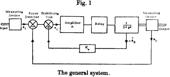
Fig. I

The general system.

The operation of such an optimum relay switching system is derived under the following assumptions.

(i) Inputs limited to step functions.

(ii) Instantaneous switching on the change-over boundary.

(iii) No time delays present in the system.

These ideal conditions are seldom satisfied in practice and the system, in general, will have to be modified even to give very nearly optimum response. Such modifications to give nearly optimum response under the non-ideal conditions cannot easily be derived, analytically.

The purpose of this paper is to show the qualitative nature of the deterioration in performance of the bang-bang system under non-idea.l conditions and to demonstrate the superiority of the saturating ser'\7o under such conditions. The magnitude of the resulting limit cycle in the case of the bang-bang servo under such conditions is calculated.

§2. THE OPTIMUM SYSTEM

[image:57.418.92.368.212.337.2]

ee=A(Bi- Bo-KvBo}

or

eelA= -x-KvY on the phase plane. (x=Bo, y=Oo).

The position of the relay which turns on maximum acceleration in one direction or other depends on the sign of (-x-KvY).

Fig.2

~'alon (Ii)

Roaion (I)

Slope ...

i-v

x

The optimum switching boundary.

If a is the maximum torque developed by the motor, then maximum acceleration isa1T2:

00

=

±a/T2 =(a/T2) sign(ee)

dy

I

.

ydx =(a T2)SIgn(ee).

}

(1)

or

Integrating, we get:

y2_Yo2= (2aIT2)(x-xo) sign (ee). (2)

Equation (2) represents a family of parabolas on the phase-plane. In fig. 2, ABC is a typical trajectory on the phase-plane. Ifthe response is not to overshoot, then eqn. (2) becomes:

yl- ±2ax/TI; (3)

- ylyl 2ax jT2

S=

ylyl

+2axjT2 =

o.

I

(4) or

Equation (4) is the parabolic switching curve;

for S<0, the output of the relay is+ve. for S>0, the output of the relay is - ve ; At the point of change over B (fig.2),

xB = - hoj2, } (5)

YB= (aho/T)1/2.

Thus the change-over from acceleration to deceleration takes place on the curve S=0, at the point XB = - ho/2, for step inputs.

This optimum change-over can be achieved by mechanizing eqn. (4) by a non-linear error processing device and a linear velocity feedba.ck stabilization term which has been called the SER:ME system by West et al.

(1954).

Fig.3

-50 -40 _ 30 -20 -10 1" H! 111

Variation of response time with input.

The Total Response Time

The total response time can be calculated easily from the above equations.

Itis assumed that no overshoot is to occur (at C):

110=+a/T2 in region (i) integrating,

Oo=at/T2.

At B,

8

0=YB=atB/T2. Hence tB =yBT2/a•

Thus, from eqn. (6), it is seen that the response time is dependent on the magnitude of the input step only sincea,the maximum torque developed is a constant for a given servo motor .. The response time versus input step magnitude characteristic is shown in fig. 3.

§3. SENSITIViTY OF THE OPTIMUM SYSTEM

In any successful optimum design the achievement of the desired response and its relative insensitivity to system parameter changes or for small component imperfections is one of the basic requirements. In many applications the invariability of the response is even more important than nominal behaviour. Analysis and synthesis procedures must take account of these requirements, as far as possible.

Consider the general control process described by the equation: x=/[x(t), u(t),w), (7)

where

x

and x are state vectors,

u(t) is the control variable vector,

wis the plant parameter vector ._.

"

If

0=

J:

F(x,u)dt

is the performance index, on the basis of which the optimum uis determined, then by solving equs. (7) and (8), Uopt, in general, can be determined.

Let

(8)

UoPt(t) ='1'[x(t), w(t), tJ. (9)

The plant parameter vector w which appears in (7) seldom corresponds to the value of w used in (9), due to component inaccuracies, environment effects, etc.

From (7) and (9) we have:

x=/[x(t),{'I'[x(t), wo(t),t)}, w); (10) optimum operation requires that w=wo'

Variations in 0due to parameter variations is given by:

!:.O=O(wo, w)-C(wo, wo)· (11)

!:.C cannot be evaluated easily in general, even for small parameter variations analytically (Dorato 1963).

By experimental analysis the effect of parameter variations and other departures from the ideal conditions can be qualitatively observed.

The CfTl'I't of friction on the idenl trajectory ha!i Ix-en studied by Klu:d.,

(IH:;:l), Stout (11153), Flugg-Lotz (11153), and many others. Ideally, tho

pnoM('nc(Jof coulomb frict ion I11URt result in bringing the error rate to zero

but not the error when the steady state is reached, But it ill observed up ...-imontally that this is not true. In the presence of friction, or under highly over damped conditions, end-point oscillations as shown in fig. " 81'\'

observed. This results in a larger settling time required to reach tho

Fig.4

7

Effect of friction and hysteresis on the switching curve.

3.2. ReIllY lIystemJis and Threslwl{l

Presence of an additional time lag (as for example the motor field build-up time constant in the system of §2) or a pure time delay results in delayed switching and may produce terminal limit cycling. Ifthe time constant of the lag or the magnitude of the time delay is known, the magnitude and frequency of the limit cycle can be calculated as shown in §4.

Fig.5

atM.b11iaation

non·linear error processing device

.N.

Re1a.r

NZ

(I 1

Input _Output

lIotor

The optimum system.

§4. STABILITY ANALYSIS

The optimum system of §2can be represented by the block diagram of fig.5.

The stability analysis of the system of fig. 5is difficult since the two non-linearities NI and N2are not in simple cascade. Since the purpose of NI and the velocity feed-back stabilization is to satisfy eqn. (4), for purposes of stability analysis, these can be replaced by a single non -linearity satisfying the boundary eqn. (4). The equivalent system is shown in fig. 6. The non-linearity NI' can be thought of as a control computer satisfying eqn. (4). Now since NI' and N2 are in simple cascade, stability analysis is possible by the describing function technique (Douce 1963).

Fig.6

to non-optimum operating conditions that may exist.

In this section, the magnitude and frequoney of the limit cycle due to

the presence of an additional lag with the process of §2 are calculated.

Itis assumed that the system has sufficient low-pass filtering effect so that the harmonics above the fundamental may Le neglected.

The describing function of the two non-Iinearities SI' and SI is evaluatod considering them in cnscade. The non-linearity}.", introduces a phase shift to the describing function, whereas SI does not contribute to the phase shift, Let ..Y(m) he the describing function of the two non-linearities in ('fiN('adc. Let

S(m) =Rexp (i4». (I:!)

Ifx""", ('08 wi, the output of NI is a square wave of magnitude fa.

Hence the magnitude R of the describing function is:

-la

R=-.

'lTm (13)

The ph ase shift

q,

is calculated by considering the control computer. The control computer in fig. 6evaluates the control signal fle:

ee=

ylyl

+2axlTI,

if ee>O, ,\= -a,

if ee<O, ,\= +a.

The phase shift is found by evaluating the instant at which ee goes through zero. Considering one-half cycle in which

y

does not change sign.

ee=2l.11nlTIcoswt - m'wl sinl wt,

eo ....0, when 2amlT' coswt - maw'sin' wt

=

0 (1") or m1w'coslwt +2am/T'coswt -m'w'=O. (15)

Solving (15) for coswt we get:

coswt =cos 8=-l/w'm{ -a/Tt +[(a/TI)' +(w'm)l]l/1}. (16)

The phase anglo 4> of the describing function =

phase anglo at which x passes through zero - phase angle O•

•. 4>=

i

-R=sin-1{l/w'm[ -a/T'+ f(aITl)'+ (wlm)I}lil]}.

Hence

..Y(III) - (4almn)expU sin-1 [llwl.m{ - alP)' +[(aITl)' +(wtm)I]l.'1}]}. (17)

If G(jw) is the tra.nsfer function of the control process, then by Nyquist stability criterion, the limit cycle must adjust itself to satisfy the equation:

which was neglected earlier, is included in the process of §2,

G(p) =[1/{T2p2(1 +TIP)}], (19) G(jw)= [l/{-T2w2(1 +jTIW)}] (20)

or G(jw}= - (I/T2w2)(1/1 +w2TI2)1/2exp{jtan-l( -wTI)}. (21)

Hence from (18) we have:

(4a/7Tm)exp{jsin-I[(I/w2m){ -a/T2 +[(a/T2)2 +(w2m)2J1/2)]}

=w2T2(1 +w2TI2)1/2exp{jtan-l (wT1)). (22)

The amplitude and frequency of the limit cycle are 'obtained by equating the magnitudes and phase angles in (22) and solving for wand m.

This results in :

w=0'45ITI,

m=5·61a (TIIT)2.

(23) (24)

Equations (23) and (24) give the frequency and amplitude of the limit cycle, respectively.

I t is seen that the period of the limit cycle is proportional to T1and the

amplitude proportional to (T1/T)2.

Ifa pure time delay Tn is present instead of the lag of time constant

T1>p~oceeding in a similar way we can show that

w=O·485

I

Tn

and m=5·42a(TnIT)2.

Thus the period and amplitudes of the limit cycle are proportional to Tn and (TnIT)2 respectively.

§5. ANALOGUE COMPUTER STUDIES

As has been observed in §3 the bang-bang system is very sensitive to parameter variations. The deterioration in the performance of the ideal system for parameter variations is studied by simulating the system on an analogue computer. For comparison of the performances under these different operating conditions, a common performance index is necessary. In these studies the total response time required to bring the system to rest for different magnitudes of input step disturbances is chosen as the index. Since the ideal bang-bang system is the minimum response time controller, this performance index is chosen. The response time

to have till'criticnl value. \\'h(,11 the stabilizer gain factor has the critical value the change-over from accvlcrafion to deceleration takes place at exactly the half-way point, resulting in a response running into the stendy state without nny over-shoot, It is ensily seen that the critical value of the gain factor is given by:

K; (criticnl)=K1/2a,

where Kl is tho gain of the error processing non-linearity. Tho response time is measured for different magnitudes of input step,

Fig.7

,

'0

Variation of response time with input. - Theoretical bang-bang.

o

Practical bang-bang.

&. System wit h Iimiter.

The parameter chosen for variation is tho gain factor of the stabilizer, The response time is measured for gain factors other than the critical, Additional time lag representing the field build-up time constant of tho motor is included and the I"<'Hpon.'IC time is measured with the stabilizer gain factor unchanged at the critical value.

The same studies are repeated on the system with the bang-bang non-linearity replaced by a Maturating non-non-linearity or a ' limiter' with a small linear regime.

r

)0

--+----~--~~--~--~---~

_{40 se h}

c 20 30

(a)

T

•

..

10 20 10 40

(b)

Variation of response time with input.

(a) Bang-bang controller. (b) Controller with limiter. -- Critical gain factor for stabilizer.

o Critical gain factor+ 10%.

&. Critical gain factor-IO%.

Fig.9

'T

6

2·

)0 20 30 40

o

50 h )0 10 10 40

(a) (b)

Variation of response time with input.

(a)Bang-bang controller. (b) Controller with limiter. -- Ideal response.

o

With a lag 1+IT:tPwith the motor.

&. With a lag 1+~:tP with the error detector.

• _6·

bang-bang system is more sensitive to changes in the stabilizer gain factor than the system with the limiter. The response time shows an increase of about 30 to 35% in the case of the bang-bang system as compared to all increase of only 12to 15

%

for the system with the limiter, when the stabilizer gain factor is reduced from the best (critical) value by 10%. The inclusion. of the additional lag results in terminal limit cycles of considerable magnitude in addition to the great increase in the response time as can be

seen from fig. 9(a). For different values of the motor field build-up time constant Tt, the measured values of the magnitude and frequency of the limit cycle agree very closely with the calculated values using eqns, (23) and (24). Thus, for any departures from the ideal conditions, the performance of the bang-bang controller is seen to deteriorate more, both qualitatively and quantitatively.

§ 6. CONCLUSIONS

By experimental studies on an analogue computer, it has been shown. that the performance of the bang-bang controller is optimum only when the conditions obtainable are ideal. For situations where there is a likelihood of the existence of time lags and parameter variations, the saturating system gives a better response as far as the total response time is concerned. With the additional time lag, the magnitude and frequency of the resulting limit cycle for the bang-bang system have been calculated. The calculated and the observed values agree closely.

The percentage over-shoot observed is larger for the bang-bang system than for the saturating system, under the changed operating conditions, except inthe overdamped case. From fig. 9(a)and (b) it is seen that when the extra lag is added with the motor, the response time increases by nearly 45 to 50% for the bang-bang system as compared to the increase of onlv

3to 4

%

for the saturating system. ~

ACK!\OWLEDGMENTS

The author is grateful to Dr. J. L.Douce for his constant guidance and

encouragement during the course of this work. The author is also grateful to the Commonwealth Scholarship Commission ofU.K.for having provided the opportunity to undertake research in this country.

REFERENCES

DORATO, P., 1963,Trans. Amer. Inst. elect. electron. Engrs, AC 8,256.

DOUOE, J. L., 1963,An Introduction to Matherrw,tics of Servomechanisms (English

Universities Press). ,. .

FLUGG-LoTZ, I., 1953, Discontinuous A utomatic Control (Princeton University

Press).. , . , •

GRAHAM, D., and l\ICRUER, D., 1961,Analysi8 of Non-linear Control Sy.~/em ...

NEISWANDER, R. S., and 11AcNEAL, R. H., 1953, Trans. Amer. Inst. elect. Enqre, 72.262.

STOUT, T.M., 1953, Trans. Amer. Inst. elect. Enqr«, 72,329.

WEST, J. C.,DOUCE, J. L.,and NAYLOR, R., 1954, Proc. Instn elect. Engrs, 101,

166.

WEST, J.C., and NIKIFORUK, P. N., 1956, Trans. Amer. Inst. elect. Enqre, 75.

PAR

T

II

SELF-OPTIMISATION

USING

PSEUDO-RANDOM BINARY SEQUENCES

SUMMARY

In this part of the thesis9 self-optimisation of

control systems by the Hill-climbing technique using

pseudo-random binary sequences as the perturbation

signal is studied. Two methods of closing the

adaptive'loop are examined.

In the first method. adjustments to the parameter

are made discontinuously once every period of the

binary sequence. The step change in parameter after

every adjustment sets up transients in the response

of the process which will in general be correlated

with the perturbing signal. The correlation of the

transient with the perturbation signal pr~duces

errors in the measured gradient during the subsequent

periods. It is shown that this error produces

dis-similar adaptive loop response from each side of the

optimum.

In the second method of closing the loop, the

*

by using a running averager • the gradient can be

measured continuously. thus resulting in a system

with continuous adjustment. Theoretical and

experi-mental responses for the two systems have been

obtained. It is shown that pontinuous parameter

adjustment reduces the effect of the transient to a

great extent resulting in similar forms of loop

,response from either side of the optimumo

The response of the system with continuous

adjustment is shown to be superior in regard to

response timev stability and errors due to output

noise disturbances when compared with the response

of the system with discontinuous adjustment.

An analogue running averager is developed which

is novel and inexpensive. The principle of operation

and performance of this running averager is described.

In a search for new uncorrelated periodic binary

sequences with a desired auto-correlation function.

two methods of synthesising these sequences are discussed.

Some new sequences have been derived.

*

A running averager

.

f

t

~(t) = x(s) ds

. t-TI

is defined as giving a response

LIST OF PRINCIPAL SYMBOLS

yet) = Response function of the controlled process.

x(t) = The per~rbation signal (PRBS).

h(~)

=

Impulse response of the process from

parameter to performance measure.

¢xy(~) = Cross-correlation function between

x(t) and yet) for a delay of ~.

K = Parameter being adjusted in the adaptive

system.

¢xx(~)

=

Auto-correlation function of x(t) for a

delay of ~.

~

=

Gradient of the parameter-performance

characteristic.

A

=

Clock period of the PRBS, Basic clock

interval.

T = Period of the chain code.

Wc

=

Repetition frequency of the PRES.

N = Number of bits in the chain code or

Set)

=

SeT) =

ret) =

z(t)

=

Zl(t) =

binary sequence.

Slope or gradient at time t.

Slope evaluated at intervals T.

Running average of x(t).

Output signal of the integrator.

due to the transient in yet).

,

z

(t) = Output signal of the second running

averager RA2.

,

Zl(t) = Error term in the measured gradient in

the system with continuous adjustment.

= rth adjustment step.

Transient factors in the system with

=

discontinuous adjustment.

g = Gradient at the working point.

q(t) = Unit step response from parameter to

performance index.

Ti = Time 'constant of an integrator.

TI = Time over which running average is taken.

Time constant of the plant.

=

Measurement time.

¢

= Phase angle of the running average

wave-form.

~'~k = Transient factors in the system with

continuous adjustment.

&K

r

G

2

~c

~ 2

nn

net)

= rth step change in parameter.

= Loop gain.

= Mean square value of the chain code.

Mean square value of the signal net).

=