An Overview of Personal Credit Scoring: Techniques
and Future Work
Xiao-Lin Li, Yu Zhong
School of Management, Nanjing University, Nanjing, China Email: [email protected]
Received May 22, 2012; revised August 23, 2012; accepted September 3,2012
ABSTRACT
Personal credit scoring is the application of financial risk forecasting. It becomes an even important task as financial institutions have been experiencing serious competition and challenges. In this paper, the techniques used for credit scoring are summarized and classified and the new method—ensemble learning model is introduced. This article also discusses some problems in current study. It points out that changing the focus from static credit scoring to dynamic behavioral scoring and maximizing revenue by decreasing the Type I and Type II error are two issues in current study. It also suggested that more complex models cannot always been applied to actual situation. Therefore, how to use the assessment models widely and improve the prediction accuracy is the main task for future research.
Keywords: Credit Scoring; Ensemble Learning; Dynamic Behavioral Scoring; Type I and Type II Error
1. Introduction
Financial risks continue to spring up in the financial markets during the past decade, which brings huge losses to financial institutions. As a result, financial risk fore- casting becomes an even more important task today. Personal credit scoring is an application of financial risk forecasting to consumer lending. It includes credit scor- ing and behavioral scoring, both of which are the tech- niques to help organizations decide whether or not to grant credit to consumers who apply to them [1]. Credit scoring determines whether the applicants is qualified while behavioral scoring decides how to deal with exist- ing customers, such as should the firm agree to increase his credit limit or what actions it will take if the customer starts to fall behind in his repayments. In fact, credit scoring is a problem of classification, whose purpose is to make a distinction between “good” and “bad” custom- ers. The banks should extend credit to “good” ones in order to increase the revenue and reject “bad” ones to avoid economic losses.
In 1941, David Durand [2] was the first to recognize ones should differentiate between good or bad loans by measurements of the applicants’ characteristics. After that, credit analysts in financial companies and mail order firms decide to whether to give loans or send merchan-dise. These rules were summarized and then used by non-experts to help make credit decisions—one of the first examples of expert systems. The arrival of credit cards in the late 1960s made the banks and other credit card issuers begin to employ credit scoring. The useful-
ness of credit scoring not only improves the forecast ac-curacy but also decreases default rates by 50% or more. In the 1970s, completely acceptance of credit scoring leads to a significant increase in the number of profes-sional credit scoring analysis. By the 1980s, credit scor-ing has been applied to personal loans, home loans, small business loans and other fields. In the 1990s, scorecards were introduced to credit scoring.
Up to now, three basic techniques are used for credit granting—expert scoring models, statistical models and artificial intelligence (AI) methods. Expert scoring method was the first approach applied to solve the credit scoring problems. The analysts said yes or no according to the characteristics of the applicants. These credit rating ap-proaches are quite similar. They all make qualitative analysis by scoring the main factors of the credit, such as moral quality, repayment ability and the collateral of the applicants, the purpose and deadline of the loans. How- ever, this method is highly dependent on the experience of experts and their tacit knowledge, which makes it a time-consuming task and brings fatigue and classification error.
In Section II, we will review four kinds of credit scor- ing methods: statistical methods, artificial intelligence methods, hybrid methods and ensemble methods. Re- search issues and future problems will be discussed in Section III. Part IV is a conclusion of this paper.
2. Overview of the Techniques
methods for credit scoring. At present the main research direction has changed from single model into integrated models. So classifying these methods has become a complex and difficult job. In this paper, we sums up these methods and classify them into statistical model, AI model, hybrid methods and ensemble methods.
2.1. Statistical Model
2.1.1. LDA
LDA (linear discriminate analysis) was first proposed by Fisher [3] as a classification method. LDA uses linear discriminate function (LDF) which passes through the centroids of the two classes to classify the customers. The linear discriminate function is following:
0 1 1 2 2 n n
LDF a a x a x a x (1) where x1 xn represents feature variables of the cus- tomers and 1 indicates discrimination coeffi-cients for n variables. LDA is the most widely used sta-tistical methods for credit scoring. However, it has also been criticized for its requirement of linear relationships between dependent variables and independent variables and the assumptions that the input variables must follow Normal distribution. To overcome these drawbacks, Lo-gistic regression, a model which not requires the normal distribution of variables, was introduced.
n
a a
2.1.2. Logistic Regression
Logistic regression (LR) is a further deformation of li- near regression. It has less restriction on hypothesis about the data and can deal with qualitative indicators. LDA analysis whether the user’s characteristic variables are correlation, while Logistic regression has the ability to predict default probability of an applicant and indentify the variables related to his behavior. The regression equation of LR is:
0 1 1 2 2
ln
1 i
n n i
p
x x x
p
(2)
The probability i obtained by Equation (2) is a bound of classification. The customer is considered de- fault if it is larger than 0.5 or not default on the contrary. Lin [4] suggested that it is not appropriate to adopt 0.5 as the cutoff point when the number of training samples in two groups is imbalance. He used optimal cutoff point approach and cross-validation to construct a financial distress warning system and get the new cut point 0.314 for classification. LR is proofed as effective and accurate as LDA, but does not require input variable to follow normal distribution.
p
2.1.3. MARS
MARS (multivariate adaptive regression splines) is a
non-linear and non-parametric regression method first proposed by Friedman [5]. It has strong generalization ability and excels at dealing with high-dimensional data. The optimal MARS model is selected in a two-stage process. In the first stage, a very large number of basis fuctions are constructed to over fit the data, which can be continuous, categorical and ordinal. In the second stage, basis functions are deleted in the order of least contribu- tions using the generalized cross-validation (GCV) crite- rion. A measure of variable importance can be assessed by observing the decrease in the calculated GCV when a variable is removed from the model. This process will continue until the remaining basis functions all satisfying the pre-determined requirements. The GCV can be ex- pressed as follow
2
21 ˆ
LOF GCV
1 ˆ
1 M
N
i M i i
f M
C M
y f x
N N
(3)where there are N observations, and C(M) is the cost- penalty measures of a model containing M basis func- tions. The numerator indicates the lack of fit on the M
basis function model fM(xi) and the denominator denotes the penalty for model complexity C(M). The MARS func- tion is usually represented using the following equation
0
,
1 1
ˆ M Km
m km v k m km m i
f x a a s x t
(4)where, a0 and am are parameters, M is the number of basis functions, Km is the number of knots, skm takes on values of either 1 or –1 and indicates the right/ left sense of the associated step function, is the label of the independent variable, and km indicates the knot location. Unlike LDA and LR, MARS does not presume that there is a linear relationship between de- pendent variable and independent variables. In addition, MARS is superior to artificial intelligence methods be- cause of short training time and strong intelligibility. As a result, MARS is usually used as a feature selection technique for classifier in hybrid models in order to ob- tain the most appropriate input variables.
,v k m
t
2.1.4. Bayesian Model
Bayesian classifiers are statistical classifiers with a “white box” nature. It can predict class membership probabilities, such as the probability that a given sample belongs to a particular class. Bayesian classification is based on Bayesian theory, which is described below. Given the training sample set D
u1, , uN1 : ,
, the task of the classifier is to analyze these training sample set and de-termine a mapping function f
x , xn
C,
1, , n
x x x . Bayesian classifiers choose the class which has greatest posteriori probability P c x
j 1, , xn
as the label, according to minimum error probability crite-rion (or maximum posteriori probability critecrite-rion). That is, if
1, , max i
j i
P c x P c x
j
, then we can determine that x belongs to i.Naive Bayes and Bayesian belief networks are two commonly used models. Naive Bayesian classifier as- sumes that the attributions of a sample are independent. Although it simplifies the calculation, the variables may be correlated in reality. Bayesian belief network is a graphical model and allow class conditional independen- cies to be defined between subsets of variables. Belief network is composed of two parts: a directed acyclic graph and conditional probability tables. Sarkar & Sriram [6] as well as Sun & Shenoy [7] found that Bayesian classifier achieved a high accuracy for prediction.
c
2.1.5. Decision Tree
Decision tree method is also known as recursive parti- tioning. It works as follows. First, according to a certain standard, the customer data are divided into limited sub- sets to make the homogeneity of default risk in the subset higher than original sets. Then the division process con- tinues until the new subsets meet the requirements of the end node. The construction of a decision tree process contains three elements: bifurcation rules, stopping rules and the rules deciding which class the end node belongs to. Bifurcation rules are used to divide new sub sets. Stopping rules determine that the subset is whether or not an end node. C 4.5 and CART are the most two common methods of credit evaluation.
2.1.6. Markov Model
Markov model uses history data to predict the distribu- tion of population in a time point at regular intervals. It speculates the trend of a population based on the regula- tion of population changing in the past. Liu, Lai & Guu [8] used a hidden Markov model and Fuzzy Markov Model respectively for risk assessment. Wang et al. [9] constructed a Markov network for customer credit eva- luation. Frydman & Schuermann [10] presented a mixing Markov model based on two Markov chains for company ratings.
2.2. Artificial Intelligence Methods
LDA and LR are two effective statistic methods. How- ever, Thomas [1] indicated that the classification accu- racy of the two models was not very high. With the rapid development of machine learning, more and more Artifi- cial Intelligence methods are applied for credit scoring, such as artificial neural networks (ANN), genetic algo- rithm (GA) and support vector machine (SVM).
2.2.1. Artificial Neural Networks
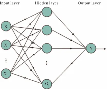
ANN is an information processing model resembling connections structure in the synapses. It consists of a large number of nodes (also called neurons or units) by links. The feed-forward neural network with back-propa- gation (BP) is widely used for credit scoring, where the neurons receive signals from pre-layer and output them to the next layers without feedback. Figure 1 shows a
standard structure of a feed-forward network, which in-cludes input layer, hidden layer and output layer. The nodes in input layer receive attributes values of each training sample and transmit the weighted outputs to hidden layer. The weighted outputs of the hidden layer are input to unit making up the output layer, which emits the prediction for given samples.
Back-propagation learns by iteratively processing a set of training samples, comparing the network’s prediction for each sample with the actual known class label. For each training sample, the weights are modified so as to minimize the mean squared error between the network’s prediction and the actual class. The modifications are made in the “backwards” direction, so we name the net- work back-propagation.
Various activation functions can be applied in hidden layer, such as logistic, sigmoid and RBF. RBF is the most common activation function. It is non-negative and non-linear, a center symmetrical attenuation local distri- bution function. There are three parameters in RBF: the center, variance and weight of the input units. The weights are obtained by solving a linear equation or using least square method recursion, which makes the learning speed faster and void the problem of local minimum point.
Figure 1. The structure of the neural network.
Figure 2. Linear separation of two classes –1 and +1 in two- dimensional space.
systems outperformed MDA.
2.2.2. SVM
SVM (support vector machine) is a new AI method for pattern classification which developed in recent years. SVM is suitable for small samples and doesn’t limit the distribution of data. Moreover, it is based on structural risk minimization (SRM) rules which ensure a good ro-bustness theoretically. Figure 2 is an example of SVM.
Let S be a dataset with M observations:
, n; 1, 1 , 1, 2,
i i i i
x y x R y i M , where xi z
denotes corresponding binary class label, indicating whether the costumer is default. The principle of SVM classification is to find a maximal margin hy-perplane to separate examples of opposite labels. The constraint can be formulated as:
1, 1i
y
,
1 0, 1, 2,i i
y w x b i M (5)
where and denotes the plane’s normal and inter- cept respectively.
w b
,
w b denotes the linear product. The
margin of separation is 2 w after normalizing the classification equation. The optimal hyperplane is ob- tained by maximizing the margin 1 2 w2, subject to the constraints of Equation (5). Then the classification pro- blem is to solve the following quadratic program;
2 ,
min 1 2
. , 1 0, 1, 2,
w b
i i
w
.
s t y w x b i M (6)
By introducing Lagrange multipliers
1, 2, , M
, the problem is transformed to solv- ing the following dual program :
1 1
1
1
max ( ) ,
2
. 0, 0, 1, 2, .
M n
i i j i j i
i i
M
i i i
i
Q y
s t y i M
j
y x x
(7)
i
x is called support vector if the corresponding . The decision function obtained by the above problem can be written as:
0
i
1 sgn , sgn M i i i,
i
f x w x b
y x x b
(8)
The decision function shown above indicates that the SVM classifies examples as class +1 if w x, b 0 and class –1 if w x, b 0.
If the classification problem is linear non-separable, we need to map the input vectors into a high-dimensional feature space via an priori chosen mapping function . The mapping can be computed implicitly by means of a kernel function K x x
i, j
xi
xj . Linear and polynomial model with degree d, sigmoid and RBF ker- nel functions are four kinds of kernels. The training er- rors are allowed in linear non-separable case. The so- called slack variables i are thus introduced to Equa- tion (5) in order to be tolerant of classification error.There are many researches on credit scoring using SVM method. Huang, Chen & Hsu [14] pointed out that SVM was superior to ANN in aspect of classification accuracy. Lee (2007) found that SVM was better than MDA, CBR and ANN models. Yang [15] (2007) pre-sented an adaptive scoring system based on SVM, which was adjusted according to an on-line update procedure. Kim & Sohn [16] (2010) provides a SVM model to pre-dict the default of funded SMEs.
2.2.3. Genetic Algorithm and Genetic Programming
Figure 3. The representation of GP tree.
land [17] from Michigan university of American in 1975. The main principle of GA can be expressed as follows. According to the evolution theory of “survival of the fittest” and beginning from the initial generation popula- tion, some genetic operations including selection, cross- over and mutation are applied to screen individuals and generate new populations visa pre-determined fitness function. This process continues until the fitness func- tions achieve greatest value and obtain final optimal so- lution. Every population is consisted of several geneti- cally-encoded individuals which are in fact chromo- somes.
One of the most important issues of applying GA to credit evaluation is fitness function. A common one can be written as follows:
1 2
1 2
1 n n
f M k
m m
(11) where n1 and n2 denote the number of misclassification of two types respectively and m1 and m2 denote the number of samples. n1/m1 and n2/m2 denotes the Type I and Type II classification error. In fact, Type II will bring greater losses so we set a constant k to control it, where k is usu- ally an integer greater than 1. In addition, M is a magni- fication factor which ensures that the fitness function can change obviously.
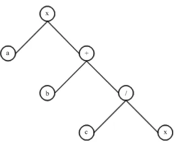
Genetic Programming (GP) is developed by Koza [18] (1992). The basic theory of GP is the same as GA. Under GP, each generation of individuals are organized through a dynamic tree structure, which can be expressed as Fig-ure 3: a
b c x
. Individual terminator set and func- tion set are particular parameters in GP. The former in- cludes both input and output variables as a, b, c, x in the figure. While the latter is used to connect leaf nodes to an individual tree, which is a potential solution of a vector. Function sets can include arithmetic operators, mathe- matical functions, boolean operators, conditional opera- tors and so on. Abdou [19] (2009), and Ong, Huang & Tzeng [20] (2005) used GP to establish a credit evalua- tion model.
GA is self-adaptive, global optimal and implicit paral- lelism. It demonstrates strong robustness and solution skills and can also be able to search global optimization in a complex space. Due to its evolutionary characteris- tics, GA does not need understand the inherent nature of a problem so that it can handle any form of objective function and constraints, no matter whether they are li- near or nonlinear, continuous or discrete.
2.2.4. K-Nearest Neighbor
K-nearest neighbor classifiers are based on learning by analogy. The training samples are described by n-dimen- sional numeric attributes. Each sample represents a point in an n-dimensional space. When given an unknown sample, a k-nearest neighbor classifier searches the pat- tern space for the k training samples that are closest to the unknown sample. The distance between two samples is defined in terms of Euclidean distance:
21
, n i i
i
d X Y x y
(12)The unknown sample is assigned the most common class among its k-nearest neighbors. Arroyo & Maté [21] (2009) combined K-nearest neighbor and time series his-togram for forecasting. K-nearest neighbor is in fact a cluster method. Except for K-nearest neighbor, SOM is also a cluster model for credits coring [22]. Luo, Chen & Hsieh [23] built a new classifier called Clustering-laun- ched Classification (CLC) and found it was more effec- tive than SVM.
2.2.5. Case-Based Reasoning
CBR classifiers are instanced-based and store problem resolution of classification. When comes to a new issue, CBR will first check if an identical training case exists. If one is found, then the accompanying solution to that case is returned. If no identical case is found, then CBR will search for training cases that are similar to the new case and find the final solution.
2.3. Hybrid Models
expectation-maximization algorithm EM). The result showed that EM + LR, LR + ANN, EM + EM and LR + EM are the optimal one of the above models respectively. In this paper, we classify hybrid models into simple hy-brid and class-wise classifier.
2.3.1. Simple Hybrid Models
In order to illustrate this issue clearly, we divide the pro- cess of building a credit evolution model into three steps: feature selection, determination of model parameters and classification. Simple hybrid approach means choosing different methods in these three stages. Feature selection plays an important role. It restricts the number of input features to improve prediction accuracy and reduce the computational complexity. Due to a better robustness and explanatory ability, statistical methods are often used for feature selection. It has been proved that ANN and SVM are the most two effective classifiers therefore both of them are applied in classification stage. Besides, GA and PSO algorithm are used as optimization method to de-termine model parameters. The simple hybrid modes based on ANN or SVM are listed in Table 1.
ANN classifier always uses statistical methods and GA for feature selection.Šušteršičet al. [26]compared three hybrid models: GA + NN, PCA + NN, LR + NN and found that GA + NN Model is superior to the other two models.
There is anther critic issue, determination of the pa-rameters, for SVM-based hybrid method. RBF is the most widely used in SVM applications. Except for pen-alty factor C it exhibits one additional kernel parameter γ, which determines the sensitivity of the distance mea- surement. Other algorithms like GA, grid algorithm and PSO are also used for feature selection and parameter selection. Among them, PSO is a new optimization me- thod developing in recent years, which can not only op- timize the parameter in RBF but also control Type II error by choosing an appropriate particle fitness function.
[image:6.595.58.286.569.738.2]
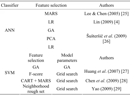
Table 1. Simple hybird methods based on ANN or SVM.
Classifier Feature selection Authors
MARS Lee & Chen (2005) [25]
LR Lin (2009) [4]
GA
PCA ANN
LR
Šušteršičet al. (2009) [26]
Feature selection
Model
parameters Authors GA GA
F-score Grid search Huang et al. (2007) [27] CART + MARS Grid search Chen et al. (2009) [28] SVM
Neighborhood
rough set Grid search Yao (2009) [29]
2.3.2. Class-Wise Classifier
There exists anther type of hybrid models: “class-wise” classifier. The information and data collected by credit institutions are often not complete. One solution is to cluster the samples automatically and decide the number of labels before classification stage. That’s why it is called “class-wise” and class-wise classifier is consistent with cluster + classification model proposed by Tsai & Chen [24]. Hsieh & Huang [30] built a clustering-classi- fier which integrates SVM, ANN and Bayesian network. Hsieh [31] established such a model for credit scoring. He first used SOM clustering algorithm to determine the number of clusters automatically and then used the
K-means clustering algorithm to generate clusters of samples belonging to new classes and eliminate the un- representative samples from each class. Finally, in the neural network stage, samples with new class labels were used in the design of the credit scoring model.
2.4. Ensemble Classifier
Ensemble learning is a novel machine learning technique. There is no clear definition of ensemble learning. It is generally believed that one of the most important charac- teristics of ensemble learning is it’s learning for the same problem, which is different from the way obtaining the overall solution from individual solution by solving seve- ral sub-problems respectively. The important difference between hybrid methods and ensemble methods is that hybrid methods only use one classifier for sample learn-ing and employ different way in feature selection and classifying stages, while ensemble learning produce various classifier with different types or parameters, such as various SVM classifiers with different parameters, and train different samples for many times .
deal with the issues of missing data and imbalance classes and perform better classification ability and per- dition accuracy compared with signal or simple hybrid models.
3. Current Research Issues
Although personal credit evaluation has become a mature research field, there still exist many problems. Building personal credit scoring models faced many challenges in reality, such as half-baked applicant’s information, miss- ing values and inaccurate information. In this section, we will discuss some issues of research problems and future research directions in this field.
3.1. Behavioral Scoring
At present, researchers seldom focus their attention on behavioral scoring. Behavioral scoring makes a deci- sion about credit management based on the repay per- formance of existing customers during a period of time. Behavioral scoring includes not only basic personal in- formation but also repayment behavior and purchasing history. Therefore, it is a dynamic process which decides whether to increase credibility and refuse or provide extra loans to costumers according to their credit perform- ance. Behavioral scoring is a dynamic process while credit scoring can be reviewed as a static process which deals with only new applicants. Thomas (2000) [1] has introduced a dynamic systems assessment model for be- havior scoring, which may become a research trend in future. Hsieh (2004) [36] established a two-stage hybrid model based on SOM and Apriori for behavior manage- ment of existing customers in banks. First, SOM was used to classify bank customers into three major profit- able groups of customers: revolver users, transactor users and convenience users based on repayment behavior and recency, frequency, monetary behavioral scoring predi- cators. Then, the resulting groups of customers were pro- filed by their feature attributes determined using an Apripri association rule inducer.
3.2. Type I and Type II Error
Type I and Type II are two kinds classification error of scoring system. For banks, Type I error classify good customer as bad one and reject their loans, which will reduce banks’ profit. In contrast, Type II error classify bad customer as good one and provide loans, which will bring loss to banks. The researches focus more on Type II error because it is generally believed that it may bring about more serious damage to credit institutions. In addi- tion, Type II error is also a criterion to evaluate a credit model. SVM is considered having an advantage over ANN because that its fitness function has the ability to
control Type II. However, it should not been ignored that reducing Type I can also cause an increase in revenue. Chuang and Lin (2009) [37] presented a reassigning credit scoring model (RCSM) in order to decrease Type I error. First they used ANN to classify applicants as ac- cepted good or rejected bad credits. Then the CBR-based classification technique was used to reduce Type I error by reassigning the rejected good credit applicants to con-ditional accepted class and provide a certain amount of loans to them. In short, how to decrease losses and at the same time maximize the revenues is a major research direction in future work.
3.3. The More Complex a Model, the Better the Classifier?
The number of credit scoring models becomes larger and each one has its own advantages. Although multi-model hybrid method and ensemble learning models is the re- search trend, credit score is still the widespread way to decide whether grant credit to applicants or not. The is- sues of application and promotion of these credit scoring models may face challenges in the future. Angelini (2008) [38] pointed out that future work should focus on models’ generalization capability and applicability. On one hand, hybrid and ensemble models which integrate advantages of different methods obviously perform higher classifica-tion accuracy. However, whether classificaclassifica-tion accuracy should be the only evolution criterion is still doubtful. On the other hand, new models are getting more complex and difficult, while the implementation cost of these models becomes much higher. Credit scoring cards and logistic regression are still the widely-used methods for credit scoring.
3.4. Incorporate Economic Conditions into Credit Scoring?
Credit scoring belongs to financial activity. In the finan- cial area, it is impossible that all the situations are as the same as what people have predicted. Forecasting also has its limitation [39]: (1) chaotic limitations. It means that our present knowledge is limited and may not correct; (2) stochastic limitations. It means that the random situation is unpredictable and this compels us to take economic condition into account when taking part in financial ac-tivities. In short, economic condition has an effect on the evolution criterion of credit institutions. When economic condition is in depression, it is suggested that evolution criteria should be properly lenient to increase the revenue of credit institutions.
4. Conclusion
up various techniques used for credit risk evolution. It credit scoring methods into statics models, AI models, hybrid methods and ensemble methods. Ensembled learn- ing has been widely applied to personal credit evolution and has better classification ability and prediction accu- racy. At last, several main issues in the process of build- ing models have been discussed in this paper. In a con- clusion, the widespread application and improvement in predication accuracy is the research trends in this field.
REFERENCES
[1] L. C. Thomas, “A Survey of Credit and Behavioral Scor-ing: Forecasting Financial Risk of Lending to Consum-ers,” International Journal of Forecasting, Vol. 16, No. 2, 2000, pp. 149-172.
doi:10.1016/S0169-2070(00)00034-0
[2] D. Durand, “Risk Elements in Consumer Instatement Financing,” National Bureau of Economic Research, New York, 1941.
[3] R. A. Fisher, “The Use of Multiple Measurements in Taxonomic Problems,” Annuals of Eugenices, Vol. 2, No. 7, 1936, pp. 179-188.
[4] S. L. Lin, “A New Two-Stage Hybrid Approach of Credit Risk in Banking Industry,” Expert Systems with Applica-tions,Vol. 36, No. 4, 2009, pp. 8333-8341.
doi:10.1016/j.eswa.2008.10.015
[5] J. H. Friedman, “Multivariate Adaptive Regression Splines,”
Annals of Statistics,Vol. 19, No. 1, 1991, pp. 1-141. doi:10.1214/aos/1176347963
[6] S. Sarkar and R. S. Sriram, “Bayesian Models for Early Warning of Bank Failures,” Management Science, Vol. 47, No. 11, 2001, pp. 1457-1475.
doi:10.1287/mnsc.47.11.1457.10253
[7] L. Sun and P. P. Shenoy, “Using Bayesian Networks for Bankruptcy Prediction: Some Methodological Issues,”
European Journal of Operational Research, Vol. 180, No. 2, 2007, pp. 738-753.doi:10.1016/j.ejor.2006.04.019 [8] K. Liu, K. K. Lai and S.-M. Guu, “Dynamic Credit
Scor-ing on Consumer Behavior UsScor-ing Fuzzy Markov Model,” 2009 Fourth International Multi-Conference on Comput-ing in the Global Information Technology, Cannes, Au-gust 2009, pp. 235-239.
[9] S. C. Wang, C. P. Leng and P. Q. Zhang, “Conditional Markov Network Hybrid Classifiers Using on Client Credit Scoring,” 2008 International Symposium on Com-puter Science and Computational Technology, Shanghai, December 2008, pp. 549-553.
doi:10.1109/ISCSCT.2008.337
[10] H. Frydman and T. Schuermann, “Credit Rating Dynam-ics and Markov Mixture Models,” Journal of Banking &
Finance,Vol. 32, No. 6, 2008, pp. 1062-1074. doi:10.1016/j.jbankfin.2007.09.013
[11] H. Abdou, J. Pointon and A. E. Masry, “Neural Nets Versus Conventional Techniques in Credit Scoring in Egyptian Banking,” Expert Systems with Applications, Vol. 35, No. 2, 2008, pp. 1275-1292.
doi:10.1016/j.eswa.2007.08.030
[12] V. S. Desai, J. N. Crook and G. A. Overstreet, “A Com-parison of Neural Networks and Linear Scoring Models in the Credit Union Environment,” European Journal of Operational Research,Vol.95, No. 1, 1996, pp. 24-47. doi:10.1016/0377-2217(95)00246-4
[13] R. Malhotra and D. K. Malhotra, “Differentiating be-tween Good Credits and Bad Credits Using Neuro-Fuzzy Systems,” European Journal of Operational Research, Vol. 136, No. 1, 2002, pp. 190-211.
doi:10.1016/S0377-2217(01)00052-2
[14] Z. Huang, H. Chen, C. J. Hsu, W. H. Chen and S. Wu, “Credit Rating Analysis with Support Vector Machines and Neural Networks: A Market Comparative Study,”
Decision Support System, Vol. 37, No. 4, 2004, pp. 543-558.doi:10.1016/S0167-9236(03)00086-1
[15] Y. X. Yang, “Adaptive Credit Scoring with Kernel Learning Methods,” European Journal of Operational Research, Vol. 183, No. 3, 2007, pp. 1521-1536.
doi:10.1016/j.ejor.2006.10.066
[16] H. S. Kim and S. Y. Sohn, “Support Vector Machines for Default Prediction of SMEs Based on Technology Credit,” European Journal of Operational Research, Vol. 201, No. 3, 2010, pp. 838-846.
doi:10.1016/j.ejor.2009.03.036
[17] J. Holland, “Genetic Algorithms,” Scientific American, Vol. 267, No. 1, 1992, pp. 66-72.
doi:10.1038/scientificamerican0792-66
[18] J. R. Koza, “Genetic Programming on the Programming of Computers by Means of Natural Selection,” The MIT Press, Cambridge, 1992.
[19] H. A. Abdou, “Genetic Programming for Credit Scoring: The Case of Egyptian Public Sector Banks,” Expert Sys- tems with Applications, Vol. 36, No. 9, 2009, pp. 11402- 11417.doi:10.1016/j.eswa.2009.01.076
[20] C. S. Ong, J. J. Huang and G. H. Tzengb, “Building Credit Scoring Models Using Genetic Programming,”
Expert Systems with Applications, Vol. 29, No. 1, 2005, pp. 41-47.doi:10.1016/j.eswa.2005.01.003
[21] J. Arroyo and C. Maté, “Forecasting Histogram Time Series with K-Nearest Neighbours Methods,” Interna-tional Journal of Forecasting, Vol. 25, No. 1, 2009, pp. 192-207.doi:10.1016/j.ijforecast.2008.07.003
[22] J. T. S. Quah and M. Sriganesh, “Real-Time Credit Card Fraud Detection Using Computational Intelligence,” Ex-pert Systems with Applications, Vol. 35, No. 4, 2008, pp. 1721-1732.doi:10.1016/j.eswa.2007.08.093
[23] S. T. Luo, B. W. Cheng and C. H. Hsieh, “Prediction Model Building with Clustering-Launched Classification and Support Vector Machines in Credit Scoring,” Expert Systems with Application, Vol. 36, No. 4, 2009, pp. 7562-7566.doi:10.1016/j.eswa.2008.09.028
[24] C. F. Tsai and M. L. Chen, “Credit Rating by Hybrid Machine Learning Techniques,” Applied Soft Computing, Vol. 10, No. 2, 2010, pp. 374-380.
doi:10.1016/j.asoc.2009.08.003
doi:10.1016/j.eswa.2004.12.031
[26] M. Šušteršic, D. Mramor and J. Zupan, “Consumer Credit Scoring Models with Limited Data,” Expert Systems with Applications, Vol. 36, No. 3, 2009, pp. 4736-4744. doi:10.1016/j.eswa.2008.06.016
[27] C. L. Huang, M. C. Chen and C. J. Wang, “Credit Scoring with a Data Mining Approach Based on Support Vector Machines,” Expert Systems with Application, Vol. 33, No. 4, 2007, pp. 847-856.doi:10.1016/j.eswa.2006.07.007 [28] W. M. Chen, C. Q. Ma and L. Ma, “Mining the Customer
Credit Using Hybrid Support Vector Machine Tech-nique,” Expert Systems with Applications, Vol. 36, No. 4, 2009, pp. 7611-7616.doi:10.1016/j.eswa.2008.09.054 [29] P. Yao, “Hybrid Classifier Using Neighborhood Rough
Set and SVM for Credit Scoring,” 2009 International Conference on Business Intelligence and Financial Engi-neering, Beijing, July 2009, pp. 138-142.
doi:10.1109/BIFE.2009.41
[30] N. C. Hsieh and L. P. Hung, “A Data Driven Ensemble Classifier for Credit Scoring Analysis,” Expert Systems with Application, Vol. 37, No. 1, 2010, pp. 534-545. doi:10.1016/j.eswa.2009.05.059
[31] N. C. Hsieh, “Hybrid Mining Approach in the Design of Credit Scoring Models,” Expert Systems with Application, Vol. 28, No. 4, 2005, pp. 655-665.
doi:10.1016/j.eswa.2004.12.022
[32] G. Paleologo, A. Elisseeff and G. Antonini, “Subagging for Credit Scoring Models,” European Journal of Opera- tional Research, Vol. 201, No. 1, 2010, pp. 490-499. doi:10.1016/j.ejor.2009.03.008
[33] L. Yu, S. Y. Wang and K. K. Lai, “Credit Risk Assess- ment with a Multistage Neural Network Ensemble Learn- ing Approach,” Expert Systems with Application, Vol. 34, No. 2, 2008, pp. 1434-1444.
doi:10.1016/j.eswa.2007.01.009
[34] L. Zhoua, K. K. Laia and L. Yub, “Least Squares Support Vector Machines Ensemble Models for Credit Scoring,”
Expert Systems with Applications, Vol. 37, No. 1, 2010, pp. 127-133.doi:10.1016/j.eswa.2009.05.024
[35] L. Nanni and A. Lumini, “An Expermental Comparison of Ensemble of Classifiers of Bankruptcy Prediction and Credit Scoring,” Expert Systems with Applications, Vol. 36, No. 2, 2009, pp. 3028-3033.
doi:10.1016/j.eswa.2008.01.018
[36] N. C. Hsieh, “An Integrated Data Mining and Behavioral Scoring Model for Analyzing Bank Customers,” Expert Systems with Applications, Vol. 27, No. 4, 2004, pp. 623- 633.doi:10.1016/j.eswa.2004.06.007
[37] C. L. Chuang and R. H. Lin, “Constructing a Reassigning Credit Scoring Model,” Expert Systems with Application, Vol. 36, No. 3, 2009, pp. 1685-1694.
[38] E. Angelini, G. D. Tollo and A. Roli, “A Neural Network Approach for Credit Risk Evaluation,” The Quarterly Re-view of Economics and Finance, Vol. 48, No. 4, 2008, pp. 733-755.doi:10.1016/j.qref.2007.04.001
[39] D. J. Hand, “Mining the Past to Determine the Future: Problems and Possibilities,” International Journal of Fore- casting, Vol. 25, No. 3, 2009, pp. 441-451.