Quantitative Evaluation of Mixing Characteristics of Static Mixers by Visualization Experiments

(1)

http://www.scirp.org/journal/jfcmv ISSN Online: 2329-3330 ISSN Print: 2329-3322

DOI: 10.4236/jfcmv.2018.61003 Jan. 3, 2018 27 Journal of Flow Control, Measurement & Visualization

Quantitative Evaluation of Mixing

Characteristics of Static Mixers

by Visualization Experiments

Noboru Mochizuki

1

, Aya Kaide

2

, Takashi Saeki

2*

1_{Business Development Department, ISEL Co., Ltd., Osaka, Japan}

2_{Graduate School of Science and Technology for Innovation, Yamaguchi University, Yamaguchi, Japan}

Abstract

We propose a convenient way of evaluating the mixing performance of static mixers used for round pipe by conducting flow visualization experiments un-der the turbulent region and using water as the main stream. A fluorescent pigment, glycerin, two carboxymethyl cellulose solutions, and rapeseed oil were each injected upstream of the mixer. Three static mixer conditions were tested: 1) no static mixer; 2) a Kenics-type static mixer; and 3) a multi-stacked elements (MSE) static mixer. The mixing trend downstream of the mixer in each condition and with each injection fluid was monitored using a laser and high-speed video camera system to obtain cross-sectional images. We propose suitable indexes based on the images obtained for quantitative evaluations of the mixing characteristics of static mixers.

Keywords

Line Mixer, Stacked Elements, Pigment, Mixing Performance, Visualization Experiment

1. Introduction

A static mixer or line mixer is a device designed to mix fluids inside a pipe. Static misers are implanted in pipes, and can divide, shear, compress, and/or replace fluids passing over a short distance; they are therefore considered space-saving equipment compared to a stirring vessel. Many types of static mixers are com-mercially available. Familiar static mixer providers include Kenics Co., Charles Ross & Son Co., and the Mixing Equipment Co. in the U.S. and the Sulzer Co. in Switzerland [1] [2]. In Japan, Noritake Co., OHR Co., Fujikin Co., and Toray

How to cite this paper: Mochizuki, N., Kaide, A. and Saeki, T. (2018) Quantitative Evaluation of Mixing Characteristics of Static Mixers by Visualization Experiments. Journal of Flow Control, Measurement & Visualization, 6, 27-38.

https://doi.org/10.4236/jfcmv.2018.61003

Received: February 1, 2017 Accepted: December 31, 2017 Published: January 3, 2018

(2)

DOI: 10.4236/jfcmv.2018.61003 28 Journal of Flow Control, Measurement & Visualization Co. offer original static mixers. Since static mixers include no driving mechan-ism, they might be energy-saving; however, insufficient mixing often occurs due to the lack of retention time. It is thus important to develop new static mixers that provide better mixing performance.

At the same time, it is necessary to develop a method for evaluating mixing characteristics quantitatively, as these data could be used both for developing new static mixers and for selecting suitable candidates. Etchells et al. [3] pro-posed using a coefficient of variation, CoV, as an index of mixing performance, which is defined as the standard deviation of the concentration distribution in the mixing field. Since the concept of the standard deviation can be applied only for a normal distribution, the numerical value and mixing image obtained by a visualization experiment could be expected to show some gaps. Alberini et al. [4] evaluated the performance of Kenics KM static mixers using two shear-thinning fluid streams in a visualization experiment. They adopted planar laser-induced fluorescence (PLIF) to obtain striation-like images at the mixer outlet by doping one fluid stream with a fluorescent dye upstream of the mixer inlet, and they then extracted the concentration distribution of the fluorescent dye. In another study, Alberini et al. proposed the areal distribution method [5], which charac-terizes individual striations by determining the distribution as a function of size and concentration. They concluded that their method gave a more consistent measure of mixing performances than the CoV. However, their experiments were conducted under only a laminar flow regimen, which allowed a characte-ristic pattern of the fluorescent dye.

In the present study, we conducted flow visualization experiments under a turbulent region using water as the main stream. Glycerin, carboxymethyl cellu-lose solutions, and rapeseed oil with a fluorescent pigment were injected up-stream of the mixer. We examined two static mixers, and proposed suitable in-dexes obtained from the cross-sectional images that enabled quantitative cha-racterization of mixing performance.

2. Experimental Procedure

2.1. Static Mixers

(3)

DOI: 10.4236/jfcmv.2018.61003 29 Journal of Flow Control, Measurement & Visualization

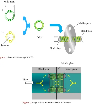
[image:3.595.164.540.70.499.2]

Figure 1. Assembly drawing for MSE.

[image:3.595.248.503.503.593.2]

Figure 2. Image of streamlines inside the MSE mixer.

Figure 3. Schematic drawing of a Kenics-type static mixer.

mixer can be used for blending under both laminar and turbulent conditions by inducing circular patterns that reverse direction at each element’s intersection.

2.2. Flow System

(4)

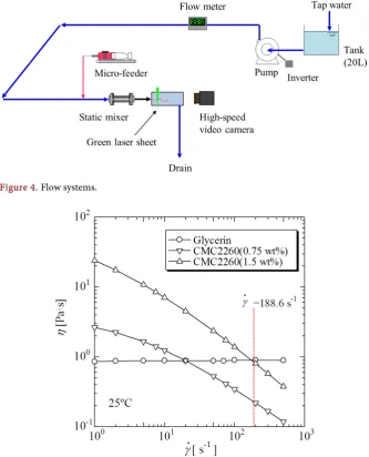
DOI: 10.4236/jfcmv.2018.61003 30 Journal of Flow Control, Measurement & Visualization flowmeter (FD-83, Keyence Co.), set at 0.5 m/s. The water temperature was 25˚C for all of the experiments. The Reynolds number was calculated as 11,700, using the diameter of the pipe as the reference length and the properties of water at 25˚C. Glycerin (Wako Co.) and carboxymethyl cellulose (CMC2260, Daicel Co.) solutions with different concentrations (0.75, 1.50 wt%), rapeseed oil (100% lipid including 7% saturated fatty acid, Nisshin Ollio Co.) were prepared as injected fluids. A fluorescent pigment, Neolan Pink B (Intracolor Co.) was added to in-jected fluids at the concentration of 1.0 wt%.

[image:4.595.207.541.293.706.2]

The flow equilibrium curves of the injected fluids measured by a rheometer (NRM-2000R, Elquest Co.) are shown in Figure 5. Glycerin and the rapeseed oil were Newtonian fluids, whereas the CMC solutions showed non-Newtonian characteristics. They were injected by a micro-feeder through a nozzle (inner dia. = 3 mm) at the center of the pipe, which was located 70-mm upstream from the inlet of the static mixers. The viscosities of the CMC solutions at the shear

[image:4.595.257.493.414.703.2]

Figure 4. Flow systems.

(5)

DOI: 10.4236/jfcmv.2018.61003 31 Journal of Flow Control, Measurement & Visualization rate equivalent to the outlet of the nozzle (=188.6 s−1_{) were 0.233 Pa·s for 0.75} wt% and 0.870 Pa·s for 1.50 wt%, respectively. The flow rate of the injected fluid was set constant at 0.1 wt% (15 cm3_{/min) with respect to the main flow.}

2.3. Flow Visualization

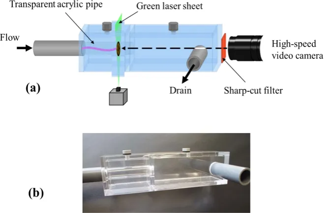
Figure 6 presents a schematic diagram and a photo of the flow visualization sec-tion set downstream of the static mixers. A transparent PVC pipe was connected just after the static mixers. The thickness of the PVC pipe was 0.2 mm, to reduce the influence of the refraction of the round pipe wall. The cross-section 180-mm downstream from the outlet of the static mixer was visualized by irradiating a 50-mW green laser sheet with a wavelength of 532 nm at a right angle to the pipe. Distribution images of the injected fluid were captured by a high-speed video camera (VW-6000, Keyence Co.) at 1/60 frames for 15 s through a sharp-cut filter, the transmission limit wavelength of which was 560 nm.

[image:5.595.210.541.490.707.2]

We converted the images (330 × 330 pixels) obtained into the quantitative values of RGB brightness (0 - 255) using ImageJ software (U.S. National Insti-tutes of Health). We then determined the correlations between: 1) the concen-tration of fluorescent pigment and R brightness; 2) the concenconcen-tration of fluores-cent pigment and G brightness; and 3) the confluores-centration of fluoresfluores-cent pigment and B brightness. The results demonstrated that the concentration of fluorescent pigment and R brightness showed a good correlation [6]. Therefore, we used R-brightness for the mixing evaluation in this study. Although G brightness also displayed good linearity, the presence of bubbles (which induced green emis-sion) always caused non-negligible errors for G brightness values. We confirmed that more than 50 images were necessary to obtain stable statistical values (er-rors of less than 5%). Therefore, we transacted 100 images for each experimental condition.

(6)

2.4. Definition of Indexes

We defined the following indexes to evaluate the mixing state of the obtained images:

1) Mixing rate: M (%)

M was defined as a spreading index, and was calculated by the number of fluo-rescent pixels divided by the total number of pixels inside the pipe cross-section (85,636 pixels). To take into account the white noise presented at the lower brightness region, the criterion of 30 for R brightness was used to judge whether or not a pixel was fluorescing. The threshold was set by comparing each R value with the corresponding pixel, and determining whether it was brightening or disappearing by viewing.

2) Extracted maximum brightness: Rmax′ (−)

max

R′ was introduced to extract highly concentrated lumps of the injected flu-id. n(R) was defined as the number of pixels for which the R brightness was R. Then, n R′

( )

was calculated using the following equation:

( )

R255

n R′ =n R

(1)

max

R′ was then determined as the R brightness at which n R′

( )

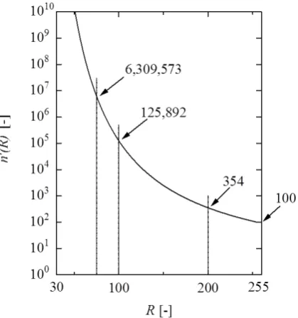
was the maximum. Figure 7 shows n R′

( )

with respect to R when n(255) = 100. The presence of 100 pixels at R = 255 is equivalent to 354, 125,892, and 6,309,573 pixels at R = 200, 100, and 75, respectively. Therefore, we could extract the presence of higher-brightness pixels.

3) Size of bright lump: L (%)

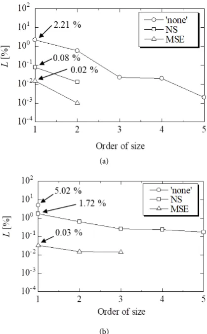
[image:6.595.271.481.475.699.2]

L was introduced to probe the presence of concentrated lumps, and we calcu-lated the rate of brighter lump pixels to total pixels. Five bright lumps in order of size were chose for each image, and L values were calculated.

(7)

DOI: 10.4236/jfcmv.2018.61003 33 Journal of Flow Control, Measurement & Visualization 4) Deviation index: Dev (−)

We obtained the center of brightness using the ImageJ image-processing pro-gram, and the value of the y-coordinate was converted to Dev. Dev was defined to express the asymmetrical presence of the vertical direction of fluorescent pix-els, where the Dev values at the top, center, and bottom inside the pipe were de-fined as 1, 0, and −1, respectively. When the density of an injected fluid was larger than water at a certain level, a negative value of Dev might be obtained.

3. Results and Discussion

Figure 8 shows typical cross-sectional images for the static mixer conditions no mixer (“none”), the Kenics type static mixer (NS), and the MSE static mixer (MSE), obtained using glycerin as an injected fluid. We can see a large fluores-cent lump located lower than the fluores-center for “none”, while mixing was performed uniformly by the NS and MES mixers.

Table 1 shows the averaged index values calculated from 100 images for each static mixer condition. The M-values > 90% demonstrate the impressive mixing performance of the two static mixers. The “none” condition also showed a high

M-value due to the high solubility of glycerin in water; however, the maximum value of Rmax′ indicates the presence of an undiluted solution of glycerin.

[image:7.595.261.485.506.583.2]

Simi-lar values of Dev among the three suggest that the density difference between glycerin and water did not affect mixing performance. With regard to L-values for “none” with glycerin, the largest lump occupied 13.39% of the total cross-section of the pipe. The second largest lump was only 0.06%, and no other lumps were confirmed. We did not observe any lumps when the NS or MSE mixers were used.

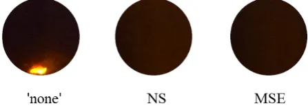
Figure 9 shows typical images for the “none”, NS, and MSE experiments ob-tained with the 0.75 wt% and 1.50 wt% CMC solutions. Since the density of 0.75 wt% CMC is almost the same as that of water, the large lump remained almost at

[image:7.595.209.538.633.719.2]

Figure 8. Cross-sectional images of “none”, NS, and MSE for glycerin as an injected fluid.

Table 1. Mixing characteristics for glycerin evaluated by three indexes.

Index Static mixer

“none” NS MSE

M (%) 64.58 97.38 96.30

max

R′ ₍₋₎ ₁₆₄ ₄₇ ₄₃

(8)

[image:8.595.272.479.67.259.2]

[image:8.595.206.539.330.563.2]

Figure 9. Cross-sectional images of “none”, NS, and MSE with CMC solutions as injected fluids: (a) 0.75 wt% CMC: (b) 1.50 wt% CMC.

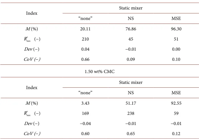
Table 2. Mixing characteristics for CMC solutions evaluated by three indexes. 0.75 wt% CMC

Index Static mixer

“none” NS MSE

M (%) 20.11 76.86 96.30

max

R′ ₍₋₎ ₂₁₀ ₄₅ ₅₁

Dev (−) 0.04 −0.01 0.00

CoV (−) 0.66 0.09 0.10

1.50 wt% CMC

Index Static mixer

“none” NS MSE

M (%) 3.43 51.17 92.55

max

R′ ₍₋₎ ₁₆₉ ₂₃₈ ₅₉

Dev (−) −0.04 −0.01 −0.01

CoV (−) 0.60 0.65 0.12

the center of the pipe without much spreading for “none”. In the NS and MSE cases, we observed that almost perfect mixing was achieved except for a few small pieces. In contrast, for the experiment using 1.50 wt% CMC solution, the difference in mixing performance between the NS and MSE mixers was clear. The concentrated solution was subdivided by the NS mixer and remained as many pieces, whereas the MSE mixer dispersed the solution uniformly over the cross-section leaving only a few pieces.

(9)

con-DOI: 10.4236/jfcmv.2018.61003 35 Journal of Flow Control, Measurement & Visualization centrations of small pieces in both images were dilute. For 1.50 wt% CMC, the

M-values indicate that the MSE showed better mixing characteristics than the NS, and our impression from these cross-sectional images supported this. The lowest value of Rmax′ indicated high-performance mixing by the MSE. The

[image:9.595.267.477.353.690.2]

rea-son for the zero Dev value for “none” can be explained by the small difference in density between water and the CMC solutions. In contrast, the swirling flow that occurred when the NS mixer was used enhanced the mixing effect, consequently showing a zero Dev value. CoV values were also calculated for each CMC con-centration and are given in the same table. Since larger values of CoV can be in-terpreted as lower mixing performance, the evaluation in the case of 0.75 wt% CMC might be reasonable. Meanwhile the mixing performance of “none” and NS were similar according to the CoV values for 1.50 wt% CMC, which showed some gaps with the image obtained by the visualization experiment. We consi-dered that CoV deviated significantly when we observed the heterogeneous exis-tence of thick threads and/or large lumps of the injected solution.

Figure 10 displays L-values in order of size for the “none”, NS, and MSE mix-ers with the different CMC concentrations. These quantitations fit the impres-sion of the mixing images obtained and shown in Figure 8.

(a)

(b)

(10)

DOI: 10.4236/jfcmv.2018.61003 36 Journal of Flow Control, Measurement & Visualization Figure 11 shows typical cross-sectional images obtained for the rapeseed oil with the fluorescent pigment as an injected fluid. The size of the droplets de-creased in the order “none”, NS, and MSE; however, the differences in the brightness of droplets among the three mixer conditions were not significant. Since rapeseed oil does not dissolve in water, fluorescent oil droplets can be ob-served in the visualization experiment, and the concentration does not reflect the brightness. The particle-size distributions of the droplets can therefore be used as an alternative to evaluate the mixing performance for water-rapeseed oil sys-tems.

Figure 12 displays the particle-size distributions of droplets obtained for the images shown in Figure 11. The 10%, 50%, and 90% pass diameters of droplets for “none”, NS, and MSE are also summarized. The lowest D50 value and the smallest difference between D10 and D90 (the sharp distribution) demonstrate the high performance of the MSE. An MSE can be used as an emulsification appa-ratus by increasing the flow rate of the main flow of water. Under these condi-tions however, the mixing fluids become clouded, which hampers the visualiza-tion experiment proposed in this study.

In this paper, we considered the mixing characteristics of static mixers by ob-serving injected CMC solutions with pigment. Although our proposed method is still a relative evaluation among various static mixers, it is an attempt to evaluate mixing characteristics quantitatively. The ability of a static mixer should be judged according to its mixing characteristics, flow resistance, cost, length, and so on.

[image:10.595.266.481.427.509.2]

Figure 11. Cross-sectional images for “none”, NS, and MSE for rapeseed oil as the in-jected fluid.

[image:10.595.209.537.552.703.2]

(11)

4. Conclusion

We conducted flow visualization experiments for NS and MSE static mixers with the goal of enabling quantitative characterization of mixing performance. The indexes of M, Rmax′ , L, and Dev were defined in this study. The quantitative

val-ues of these indexes almost perfectly coincided with the impression of images obtained of the static mixers. We found that particle-size distribution is conve-nient for evaluations of mixing performance when a non-aqueous liquid is used as an injected fluid. Our analysis of the cross-sectional images obtained from the visualization experiments showed that the MSE provided effective mixing.

Acknowledgements

The authors appreciate the experimental assistance of a student colleague (Y. Moriguchi).

References

[1] Thakur, R.K., Vial, Ch., Nigam, K.D.P., Nauman, E.B. and Djelveh, G. (2003) Static Mixers in the Process Industries—A Review. Chemical Engineering Research and Design, 81, 787-826. https://doi.org/10.1205/026387603322302968

[2] Ghanem, A. Lemenand, T., Valle, D.D. and Peerhossaini, H. (2014) Static Mixers: Mechanisms, Applications, and Characterization Methods: A Review. Chemical En-gineering Research and Design, 92, 205-228.

https://doi.org/10.1016/j.cherd.2013.07.013

[3] Etchells, A.W. and Meyer, C.F. (2004) Mixing in Pipelines. In: Paul, E.L., Atie-mo-Obeng, V.A. and Kresta, S.M., Eds., Handbook of Industrial Mixing, Wi-ley-Interscience, Hoboken, NJ.

[4] Alberini, F., Simmons, M.J.H., Ingram, A. and Stitt, E.H. (2014) Assessment of Dif-ferent Methods of Analysis to Characterise the Mixing of Shear-Thinning Fluids in a Kenics KM Static Mixer Using PLIF. Chemical Engineering Science, 112, 152-169.

https://doi.org/10.1016/j.ces.2014.03.022

[5] Alberini, F., Simmons, H.J.H., Ingram, A. and Stitt, E.H. (2014) Use of an Areal Distribution of Mixing Intensity to Describe Blending of non-Newtonian Fluids in a Kenics KM Static Mixer Using PLIF. AIChE Journal, 60, 332-342.

https://doi.org/10.1002/aic.14237

(12)