Patterns and Pricing of Idiosyncratic Volatility in the French Stock Market

(1)

ISSN Online: 2162-2086 ISSN Print: 2162-2078

DOI: 10.4236/tel.2018.81005 Jan. 29, 2018 79 Theoretical Economics Letters

Patterns and Pricing of Idiosyncratic Volatility

in the French Stock Market

Zhentao Liu

1

, Gilbert V. Nartea

2

, Ji Wu

3*

1_{Institute for Financial & Accounting Studies, Xiamen University, Fujian, China}

2_{Department of Economics and Finance, UC Business School, University of Canterbury, Christchurch, New Zealand} 3_{School of Economics and Finance, Massey Business School, Massey University—Albany Campus, Auckland, New Zealand}

Abstract

We investigate the time series behavior of idiosyncratic volatility and its role in asset pricing in France. We find that both aggregate idiosyncratic and mar-ket volatility exhibit regime switching behavior similar to that in the U.S. and other developed countries. Furthermore, we find a marginally significant neg-ative IVOL effect in the French stock market. We add new evidence to the mounting results questioning the ubiquity of the IVOL effect which highlights the importance of country verification of so called anomalies in the US, even in developed markets.

Keywords

Idiosyncratic Volatility, Regime Switch Model, Asset Pricing, France

1. Introduction

In a recent study, Ang et al.[1] confirm the ubiquity of a puzzling negative idio-syncratic volatility (IVOL) effect [1] in 23 developed countries, including the seven largest developed economies (G7) where high volatility stocks earn low risk-adjusted returns. This is puzzling because traditional finance theory sug-gests that idiosyncratic volatility should not be priced as it could be eliminated at no cost through diversification. In case investors cannot fully diversify, finance theory suggests a positive (not a negative) relationship between idiosyncratic risk and return [2][3]. Ang et al. [4] report a statistically significant difference in risk-adjusted returns between high and low IVOL portfolios of 1.31% per month across 23 developed markets.1_{However, in their study, they also report that} 1_{However, some studies suggest that Ang et al.’s findings are not robust to portfolio weighting}

schemes [5] [6] and controls for short-term reversals [7]. Others argue that a positive relationship exists between idiosyncratic volatility and returns using alternative measures of expected idiosyn-cratic volatility [8] [9] [10] [11] [12].

How to cite this paper: Liu, Z.T., Nartea, G.V. and Wu, J. (2018) Patterns and Pric-ing of Idiosyncratic Volatility in the French Stock Market. Theoretical Economics Let-ters, 8, 79-97.

https://doi.org/10.4236/tel.2018.81005

Received: July 19, 2017 Accepted: January 26, 2018 Published: January 29, 2018

(2)

DOI: 10.4236/tel.2018.81005 80 Theoretical Economics Letters

among G7 countries not only did France show a decrease in the magnitude of the idiosyncratic volatility coefficient when idiosyncratic volatility was computed using a local Fama-French model instead of a world Fama-French model, but also the idiosyncratic volatility coefficient turned insignificant, indicating the absence of an IVOL effect. We investigate this further in this study. To the best of our knowledge, this is the first paper to examine the role of IVOL in pricing French stocks. If there is no significant relationship between returns and idio-syncratic volatility in the French stock market, this would add to mounting evi-dence questioning the ubiquity of the so called idiosyncratic volatility effect [5] [6][11][13]-[19].

Campbell et al. [20] report evidence of an increasing trend in idiosyncratic volatility in the U.S. relative to market volatility in the period 1962 to 1997. This is important since it implies increasing benefits from diversification. Theoreti-cally, if there is an increasing trend in IVOL with a flat market volatility, inves-tors would benefit from portfolio diversification. If IVOL has a decreasing trend or remains flat, then it is hard for investors to capture diversification benefits. In this sense, IVOL may not be priced in the stock market. However, Brandt, Brav, Graham, and Kumar [21] dispute Campbell et al.’s findings of an increasing trend, suggesting instead an episodic pattern in idiosyncratic volatility in the U.S. that is largely driven by the behavior of retail investors. In a related study Bekaert, et al.[22] show for the U.S. and in 22 other developed markets, that in-stead of a long-term trend, IVOL follows a stationary autoregressive process that occasionally switches to a higher variance regime. The trend in IVOL is an im-portant issue relative to the benefit of portfolio diversification, hence our interest in the historical trend of IVOL in the French stock market, which is also the first evidence on this issue.

In this study, we investigate the behavior of aggregate idiosyncratic and mar-ket volatility from 1991 to 2012 in the French stock marmar-ket. Then we examine the relationship between idiosyncratic volatility and cross-sectional stock re-turns. There are two reasons why we are interested in the IVOL effect in French stock market. First, most of the previous literature investigates trends and pric-ing behavior of IVOL in a group of European stock markets, but not in the French stock market on its own. The French stock market is one of the oldest stock markets in the world, and the 2nd_{largest stock market ranked by}

capitali-zation in Europe following the U.K. stock market. Moreover, the French stock exchange was ranked the 4th_{largest exchange in the world, with a total market}

(3)

me-DOI: 10.4236/tel.2018.81005 81 Theoretical Economics Letters

dium-sized companies (the Second Marché), and the list for fast-growing start-up companies (the Nouveau Marché). In September 2000, the Paris Bourse merged with the Amsterdam, Lisbon and Brussels exchanges to form Euronext NV [24]. There are more than 1300 companies listed on the integrated exchange at moment. It would be interesting to test the IVOL effect for French listed firms only on a universal stock market after the consolidation of independent Euro-pean markets since our testing period covers both periods.

We can easily summarize our results. First, we test for the presence of trends in aggregate idiosyncratic and market volatility using Bunzel and Vogelsang’s

[25]t-dan test. We also follow Bekaert et al.’s [22] method to further test for re-gime shifts. We find that both idiosyncratic and market volatility do not exhibit long-term trends. Instead, their patterns are consistent with regime switching behavior. Second, though we initially find a significant negative IVOL effect in the French stock market which is robust in bi-variate Fama-MacBeth regres-sions, the negative IVOL effect becomes marginally significant when we control for SIZE, BM, momentum, and short-term reversal simultaneously. Our new evidence suggests that there is a marginal IVOL effect in the French stock mar-ket adding to the increasing number of studies questioning the ubiquity of the negative IVOL puzzle.

We contribute to the literature on the idiosyncratic volatility effect in a num-ber of ways. First, we present the first empirical evidence examining the trend in IVOL and its role in asset pricing in the French stock market. Prior studies mostly focused on a group of developed stock markets rather than on individual stock markets. Hence we draw attention for both academia and practitioners on an individual developed stock market. Second, we add new evidence to the mounting results questioning the ubiquity of the IVOL effect. This highlights the importance of country verification of so called anomalies in the US, even in de-veloped markets. Next, we provide empirical evidence on the pricing of IVOL both at the portfolio and firm levels. Previous research only focuses on the role of pricing IVOL on either portfolio level or firm level. Therefore, our results are comprehensive and more convincing. Finally, we confirm earlier evidence that idiosyncratic volatility in the French stock market exhibits a regime switching behavior rather than showing a long-term time trend.

The rest of the paper is organized as follows: Section 2 describes our data and methods; Section 3 presents the empirical results in three parts. First we report volatility patterns over time, then we examine the relation between volatility and market returns, and finally we examine the relation between idiosyncratic vola-tility and cross-sectional stock returns. Section 4 concludes the paper.

2. Data and Methods

(4)

pe-DOI: 10.4236/tel.2018.81005 82 Theoretical Economics Letters

riod from August 1991 with 147 firms, to June 2012 with 507 firms, with an av-erage of 443 firms per month2_{. The risk-free rate which is defined as French}

EU-FRANCE 1 month middle rate was also obtained from the DataStream. Market returns are the value-weighted returns of all firms used in the study.

We exclude investment trusts, closed-end funds, exchange traded funds, and preferred shares. At the beginning of each month, we exclude stocks that do not have continuous return records in the past 22 trading days. In order to reduce noise in computing IVOL for each stock, we also exclude stocks with daily re-turns less than −100% and/or monthly return greater than 200% as well as stocks with negative book-to-market (BM) ratio. Stocks with missing accounting data in a particular month were also excluded from the sample in that month.

2.1. Estimating Idiosyncratic Volatility

We follow Ang et al.[1][4] and estimate the IVOL of each firm at the beginning of every month. IVOL is the standard deviation of the residuals (σεi) from the

Fama-French [26] [27] 3-factor model (1), henceforth FF3-factor model, using daily data for the previous 22 trading days.

, , , , , , , ,

i t MKT i m t SMB i m t HML i m t i t

R = +α β MKT +β SMB +β HML +ε ₍₁₎

where day t refers to the 22 trading days ending on the last trading day of month

m-1. Ri,t and MKT are excess returns of firm i and the market, respectively, over

the risk-free rate. SMB is the excess return of small firms over big firms, and

HML is the excess return of high book-to-market (BM) firms over low BM firms. SMB is the return of the upper half less the return of the lower half of all firms ranked in ascending order according to market capitalization while HML

is the return of the bottom third less the return of the top third of all firms ranked in ascending order according to BM.

2.2. Portfolio Analysis and Fama-MacBeth Regressions

We use both portfolio-level analysis as well as firm-level Fama-MacBeth cross-sectional regressions to examine the relation between IVOL and expected returns. In portfolio-level analysis, firms are first sorted into tertiles at the start of each month based on IVOL and allocated to groups. We then compute each tertile portfolio’s equal- and value-weighted raw returns for the current month. We also estimate each tertile portfolio’s alpha (α coefficient) from the FF3-factor model (Equation (1)) using each tertile portfolio’s full sample of monthly value- or equal-weighted returns.

As a robustness test, we also conduct firm-level Fama-MacBeth regressions to control for various variables. We estimate the following model and its nested versions:

2_{The Appendix 1 shows the details of our sample stocks. The average numbers of share in the}

(5)

, 1 0, 1, , 2, , 3, ,

4, , 5, ,

Value

Reversal Momentum

i t t t i t t i t t i t

t i t t i t

R β β IV β SIZE β

β β

+ = + + +

+ + (2)

Rt, is realized stock return in month t. IVOL is realized idiosyncratic volatility

as defined previously. SIZE at the end of month t is defined as the log of the firm’s market capitalization at the end of month t. BM is the firm’s book-to-market ratio six months prior, i.e. at the end of t-6. Following Jegadeesh and Titman

[28], MOM at time t is the stock’s 11-month past return lagged one month, i.e.

return from month t-12 to month t-2. REV in month t is short-term reversal de-fined as the return on the stock in month t-1, following Jegadeesh [29] and Lehmann [30].

3. Empirical Results

3.1. Volatility Patterns over Time

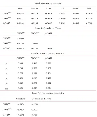
3.1.1. Descriptive Statistics

We report the descriptive statistics for three volatility series in Table 1. MVOL is monthly market volatility (MVOL). The MVOL for a given month m is the standard deviation of the daily value-weighted market returns for the past 22 trading days ending on the last trading day of month m. IVOLEW_{and IVOL}VW

are respectively the equal-weighted (EW) and value-weighted (VW) average idiosyncratic volatility across all firms, where IVOL is the standard deviation of residuals from (1). Table 1 shows that both IVOLEW_{and IVOL}VW_{are 0.0188 and}

0.0127 respectively, which is only about half compared to the IVOL in China, the biggest emerging stock market in the world [31]. The results support the view that stock markets in developed countries might be more stable than those in emerging stock markets. Moreover, the results also indicate that small firms seem to have higher idiosyncratic volatility than big firms as suggested by the higher mean of IVOLEW_{compared with IVOL}VW_{. This is consistent with results}

in other markets particularly the U.S. However, IVOLEW_{is less variable than}

IVOLVW_{as indicated by its lower coefficient of variation (CV). MVOL on the}

other hand is more variable than IVOLEW_{having a higher CV, but it has a}

simi-lar CV as IVOLVW_.

As expected, our volatility measures are highly correlated as shown in Panel B, with correlation coefficients ranging from 0.849 to 0.913.

Panel C displays the autocorrelation structure of the three volatility series. As serial correlation is fairly high in all three series, we test for the presence of unit roots using the augmented Dickey and Fuller [32] test. Panel D shows that we can reject the presence of unit roots for all three series, whether or not a trend is included. Hence our analysis of the volatility series will be in levels instead of first differences.

3.1.2. Does a Time Trend Exist?

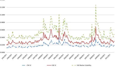
Figure 1 plots IVOLEW_{, IVOL}VW_{, and MVOL. As indicated in}_{Figure 1}_{, there}

(6)

[image:6.595.208.542.198.600.2]

Table 1. Descriptive statistics. IVOLEW_,_IVOLVW_{and MVOL, are respectively the equal-}

and value-weighted idiosyncratic volatility and market volatility. The sample period is 1991: 08-2012: 06. At the beginning of every month, we compute IVOL of each firm as the standard deviation of the residuals of the FF3-factor model by using daily return data from the previous 22 trading days. We use the standard deviation of daily value-weighted market returns for the past 22 trading days ending on the last trading day of month to represent the MVOL. The Augmented Dickey-Fuller test for unit roots in Panel D are based on regressions with a constant, and regressions with a constant and a trend. The 1% critical values for the unit root test are −3.47 with a constant, and −4.01 with constant and a trend respectively.

Panel A: Summary statistics

Mean Median Stdev CV MAX Min

IVOLEW _0.0188 _0.0174 _0.0048 _0.2553 _0.0397 _0.0120

IVOLVW _0.0127 _0.0113 _0.0043 _0.3386 _0.0322 _0.0074

MVOL 0.0184 0.0165 0.0067 0.3641 0.0582 0.0098

Panel B: Correlation Table

IVOLEW _IVOLVW _MVOL

IVOLEW _1.0000

IVOLVW _0.8528 _1.0000

MVOL 0.8489 0.9130 1.0000

Panel C: Autocorrelation structure

ρ1 0.843 0.815 0.775

ρ2 0.748 0.727 0.607

ρ3 0.702 0.681 0.504

ρ4 0.621 0.615 0.422

ρ6 0.545 0.552 0.371

ρ12 0.451 0.373 0.224

Panel D: Unit root test t-statistics Constant Constant and Trend

IVOLEW _−4.6134 _−4.6588

IVOLVW _−3.9604 _−3.9728

MVOL −5.5268 −5.5271

Instead, the plots suggest episodic behavior in these series. There was an upward trend in all three volatility series from 1991 to 2001, a downward trend until 2006, a spike in 2009 followed by a decreasing trend thereafter. The pattern of our volatility measures in Figure 1 are very similar to the volatility figures for the French stock market reported by Duncan and Kabundi [33].

(7)

[image:7.595.64.531.77.350.2]

Figure 1. Volatility Series for French Stock Market. This figure plots the monthly equal-and value-weighted idiosyncratic volatility

and the value-weighted market volatility. The sample period is 1991: 08 to 2012: 05.

0 1 2 1

t t t

VOL b b t b VOL= + + ₋ +ε ₍₃₎

where VOL represents IVOLEW_{, IVOL}VW_{, and MVOL, and}_t_{is time. The}

esti-mated time trend b1 parameter and its t-statistic are reported in Table 2. Over

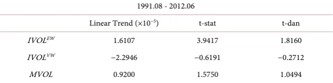
the full sample period from 1991: 08 to 2012: 06, the standard t-test shows a sta-tistically significant positive trend in IVOLEW_{but no trend for both IVOL}VW_and

MVOL. However, Vogelsang [34] points out that when errors in the trend re-gression are persistent, the student t-value often rejects the null hypothesis of no trend. As a consequence Bunzel and Vogelsang [25] developed the t-dan test which we employ in this study.3_{This test is valid whether or not a unit root}

ex-ists in the error terms. The t-dan test also has better power than the standard t-test while retaining its good size properties. The t-dan test statistics reported in

Table 2 confirm the absence of a trend in either IVOLVW_{or MVOL but a}

posi-tive trend in IVOLEW_{which indicates that the IVOL of small stocks have been}

trending upwards. However, this apparent trend in IVOLEW_{could be simply due}

to the spike in volatility towards the end of 2008. Nonetheless, the fact that MVOL and IVOLVW_{are relatively flat over the study period, implies that there is}

also no trend in correlations among stocks and that the benefits from diversifi-cation would have likely remained the same on average over the study period, which also means that the number of stocks needed to attain a certain level of diversification would also have remained the same.

(8)

[image:8.595.208.539.156.239.2]

Table 2. Time trend of volatility series. We run the following model by regressing the

vo-latility measure on its first lag and a time trend: VOL b b t b VOLt= +0 1 + 2 t−1+εt where VOL represents IVOLEW_,_I_VOLVW_{, and MVOL, and}_t_{is time. The estimated time trend}_b

1

parameter and its t-statistic and the Bunzel and Vogelsang [25] t-dan test statistic for the full sample period are reported in Table 2. The 5% critical value (two-sided) for t-dan is 1.726.

1991.08 - 2012.06

Linear Trend (×10−5₎ _t-stat _t-dan

IVOLEW _1.6107 _3.9417 _1.8160

IVOLVW _−2.2946 _−0.6191 _−0.2712

MVOL 0.9200 1.5750 1.0494

3.1.3. Regime Switching Behavior in Idiosyncratic Volatility

In this section, we test for regime-switching behavior in idiosyncratic volatility. We follow Bekaert et al.’s [22] method to further test whether or not our volatil-ity series in the French stock market is characterized by a stationary process that occasionally switches between high- and low-volatility regimes. Bekaert et al.

[22] argue that the upward trends of idiosyncratic volatility in the U.S. and 22 other developed markets were driven by the chosen starting- and ending time points. For example, if the starting point is in a low volatility period, while the end point is in a high volatility period, then the trend test would easily show a positive trend. Bekaert et al.[22] thus suggest that idiosyncratic volatility in the U.S. and 22 other developed markets are best characterized by a stationary process that occasionally switches between high- and low-volatility regimes. A regime-switching behavior in idiosyncratic volatility also appears evident in emerging markets with Nartea, et al. [35] documenting evidence of such beha-vior in the Chinese stock market, the world’s largest emerging market.

To test for regime switching behavior in idiosyncratic volatility in the French stock market, we let volatility, yt, follow an AR(1) model where all parameters

can take on one of two values depending on the realization of a discrete regime variable, st. The regime variable follows a Markov chain with constant transition

probabilities. Indexing the current regime by i the model is

(

)

1

{ }

1 , 0,1

t i i i t i t

y = −b µ +b y₋ +σe i∈ ₍₄₎

with et ~ N (0,1). In the model, we force regime 0 (regime 1) to be the low (high)

volatility regime and the mean levels (μi) of the volatility series of both regimes

to be nonnegative (i.e.μ1 > μ0 > 0).

The transition probability matrix, Φ, is 2 × 2, where each probability represents P st i st =_ − = 1 j__{, with} i j, ∈

{ }

1,2 _:

11 1 11

1 pp22 p22p

−

 

Φ =  ₋ 

 

The model has only 8 parameters,

{

µ µ0, , , , , , 11, 221 b b0 1 σ σ0 1 p p

}

.

(9)

[image:9.595.207.539.168.415.2]

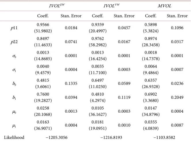
Table 3. Regime switching model estimation results. We report the regime-switching

model results for the three volatility series. The model is:

(

1

)

1 ,

{ }

0, 1

t i i i t i t

y = −b µ +b y− +σe i∈ The transition probability matrix is:

11 1 11

1 pp22 p22p

−

 

Φ = _ ₋ _ The transition probability parameters, p11 and p22, are con-strained to be in (0,1) over the study period. We also reparameterize to ensure μ2 > μ1 > 0.

The estimation period is over 1991.08 to 2012.06. T-statistics are reported in parenthesis.

Coeff. Stan. Error Coeff. Stan. Error Coeff. Stan. Error

p11 _(51.9802)0.9566 0.0184 _(20.4997)0.9359 0.0457 _(5.3824)0.5898 0.1096

p22 _(11.4633)0.8497 0.0741 _(58.2982)0.9762 0.0167 _(28.3458)0.8974 0.0317

σ0 _(14.8685)0.0013 0.0001 _(16.4254)0.0013 0.0001 _(14.7378)0.0018 0.0001

σ1 _(9.4579)0.0040 0.0004 _(11.7100)0.0035 0.0003 _(9.4864)0.0064 0.0007

b0 _(3.6061)0.4815 0.1335 _(11.0250)0.6497 0.0589 _(26.9328)0.6357 0.0236

b1 _(19.2827)0.7600 0.0394 _(4.2974)0.4810 0.1119 _(3.3680)0.6902 0.2049

μ0 _(20.1068)0.0258 0.0013 _(36.1627)0.0105 0.0003 _(34.8796)0.0147 0.0004

μ1 _(36.9071)0.0163 0.0004 _(19.0951)0.0181 0.0010 _(4.0839)0.0355 0.0087

Likelihood −1205.3056 −1216.8193 −1103.8582

to compute the standard errors. Table 3 shows that levels for both EW and VW IVOL in the low volatility regime (μ0) at 0.0258 (IVOLEW) and 0.0105 (IVOLVW)

respectively, which are both statistically significant. The corresponding levels in the high volatility regime (μ1) at 0.0163 and 0.0181 are also both statistically

sig-nificant. The differences between the levels of the two regimes for both volatility series are also statistically significant as indicated by the results of the Wald test. Our results also show higher volatility in regime 1(σ1) compared with regime 0

(σ0) for both EW and VW IVOL. The EW (VW) volatility in regime 1 is 0.0040

(0.0035) compared with 0.0013 (0.0013) for regime 0. Thus we find that idiosyn-cratic volatility in the French stock market conforms with a stationary autogressive process that occasionally switches between high and low-variance re-gimes. This is consistent with the behavior of idiosyncratic volatility in devel-oped stock markets [22] and in the world’s largest emerging market [35].

(10)

(a)

(11)

[image:11.595.211.536.104.367.2]

(c)

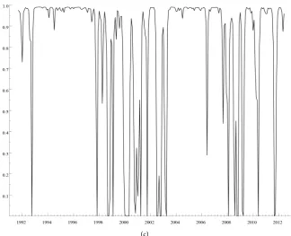
Figure 2. Smoothed probabilities of being in the low volatility regime (regime 0). The

figure shows the smoothed probability of being in regime 0 for French, using a re-gime-switching model reported in Equation (4). The model is estimated over sample pe-riod 1991 to 2012.

volatility regime from 1992 to mid-2000, consistent with Morel’s [36] findings in the French stock market. And then, it shifts to a low volatility regime until the early of 2006. Furthermore, the IVOLEW_{remained in a high volatility regime}

during the 2008 financial crisis, until the beginning of 2009 when it switched again to a low volatility regime. Panel b of Figure 2 shows that IVOLVW_switched

between high- and low volatility regimes more frequently than IVOLEW_{. IVOL}VW

stayed in the low volatility regime for most of the 20 year testing period, for ex-ample from 1992 to March 1998, January 2003 to January 2008, and September 2009 to the end of the study period. If we define yt to be in regime 0 if the

proba-bility of being in regime 0 is higher than 0.5, and vice versa for regime 1, then there are 4 regime switches in IVOLVW_{and 3 regime switches in IVOL}EW_over

(12)

the regime of IVOLVW_{reported in the panel b.}

Figure 2 confirms an insignificant time series trend in IVOL in the French stock market consistent with results reported in Table 2. For example, the ab-sence of a trend in both IVOLVW_{and MVOL reported in}_{Table 2}_{is consistent}

with both panels b and c in Figure 2, where both series start and end in the low volatility regimes over our study period. Panel a of Figure 2 shows that our test-ing period starts from a high-level of IVOL and ends in a low-level of IVOL, which indicates that the significant positive trend in IVOLEW_{reported in}_{Table 2}

is not due to the choice of sample period. However, results reported in Table 3

still suggest a significant regime-switching behavior for IVOLEW_.

We also find it interesting that IVOLVW_{and IVOL}EW_{exhibit a divergence in}

the period from 1992 to 1999, with IVOLEW_{being on a high-volatility regime}

while IVOLVW_{was on a low-volatility regime. We suggest that this could be due}

to the boom in high-tech stocks over this period. As high-tech stocks are nor-mally smaller in size and more volatile than traditional listed firms, we expect IVOLEW_{to be more volatile than IVOL}VW_{before the high-tech bubble burst}

around year 2000. We also find that both IVOLVW_{and IVOL}EW_{were on a high}

volatility regime during the recent 2008 financial crisis. This is consistent with previous findings in the literature wherein stock markets are more volatile dur-ing the financial crisis period than other periods [35]. Finally, we find that both IVOLVW_{and IVOL}EW_{show a convergent behavior after 2002 in the French stock}

market.

In sum, the results from Table 3 and Figure 2 indicate evidence of episodic behavior in all three volatility series, consistent with occasional regime shifts throughout the study period.

3.2. Can Idiosyncratic Volatility Predict Cross-Sectional Expected

Stock Returns?

3.2.1. Portfolio-Level Analysis

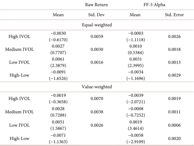
In this section we examine the presence of an IVOL effect in the French stock market. Table 4 shows the average monthly returns and FF-3 alpha of EW and VW portfolios sorted according to idiosyncratic volatility. Though both the EW and VW return spreads between high and low IVOL portfolios are consistently negative at −0.91% and −0.71% per month respectively, they are not statistically significant. We only report the FF-3 alpha of each portfolio in the third column. Stotz et al. [36] report that there are not big differences between Fama and French’s alpha and Jensen’s alpha. The EW alpha spread is likewise negative at −0.34% per month but also statistically insignificant. The exception is the statis-tically significant VW alpha spread at −0.58% per month. This appears to be consistent with the anomalous and puzzling evidence documented by Ang et al.

[1] [4] and Brockman and Yan [37] for the U.S. market. However it is not as high as the −1.31% per month reported by Ang et al. [1] for the U.S.

(13)

[image:13.595.207.539.177.426.2]

Table 4. Returns of portfolios sorted by idiosyncratic volatility. Stock portfolios have

been sorted by IVOL at the beginning of every month, i.e., high IVOL (HIV), medium IVOL (MIV) and low IVOL (LIV). The table thus reports each portfolio’s equal- and val-ue-weighted raw returns for the current month. Each portfolio’s alpha (α coefficient) is also included in the table, which is from the FF3-factor model estimated using the full sample of monthly value- or equal-weighted returns for each portfolio. The last row presents the difference in monthly raw returns and differences in alpha between the high and low IVOL portfolios. T-statistics are reported in parenthesis.

Raw Return FF-3 Alpha

Mean Std. Dev Mean Std. Error

Equal-weighted

High IVOL _(−0.6170)−0.0030 0.0059 _(−1.1118)−0.0003 0.0026

Medium IVOL _(0.7707)0.0027 0.0030 _(0.5384)0.0010 0.0018

Low IVOL _(2.3879)0.0061 0.0016 _(2.3995)0.0031 0.0013

High-Low _(−1.6526)−0.0091 _(−1.1696)−0.0034 0.0029

Value-weighted

High IVOL _(−0.3658)−0.0019 0.0070 _(−2.0721)−0.0039 0.0019

Medium IVOL _(0.7288)0.0028 0.0038 _(−0.7252)−0.0008 0.0011

Low IVOL _(1.5867)0.0051 0.0026 _(3.4614)0.0019 0.0006

High-Low _(−1.1363)−0.0071 _(−2.9109)−0.0058 0.0020

characteristics of the IVOL-sorted portfolios in Table 5. We report values for IVOL, size (SIZE), BM (Value), momentum (MOM), and short-term reversal (REV). These variables are as defined previously. The high IVOL portfolio has three times as much IVOL as the low IVOL portfolio and the difference is highly statistically significant as expected. High (low) IVOL stocks also tend to be small (big) stocks. These results are consistent with Drew et al.’s [38] findings in the German and UK stock markets, where they find that small firms have higher IVOLs than big firms. High (low) IVOL stocks also tend to be previous losers (winners) in the past 11 months. However, there is no significant difference in the value and short-term reversal variables between high and low IVOL portfo-lios. We formally control these variables using firm-level cross-sectional regres-sions in the next section.

3.2.2. Firm-Level Cross-Sectional Regressions

(14)

[image:14.595.206.538.492.638.2]

Table 5. Characteristics of portfolios sorted by idiosyncratic volatility. The table shows

that average firm’s characteristics of each IVOL sorted portfolio over the full sample pe-riod, i.e., high IVOL (HIV), medium IVOL (MIV) and low IVOL (LIV). IVOL is the standard deviation of the residuals of the FF3-factor model computed using the past 22 trading daily returns data. SIZE is the firms’ capitalization at the end of month t; Value is the firm’s book-to-market ratio six months prior, i.e. at the end of t-6. Momentum represents the stock’s 11-month past return lagged one month by following Jegadeesh and Titman [28], i.e. return from month t-12 to month t-2. REV in month t is short-term re-versal defined as the return on the stock in month t-1, following Jegadeesh [29] and Leh-mann [30]. T-statistics are reported in parenthesis.

IVOL SIZE Value Momentum REV

High IVOL _(55.7154)0.0303 _(23.9111)575.82 _(37.8627)0.8218 _(−1.5912)−0.0394 _(0.7793)0.0044

Medium IVOL _(61.3300)0.0166 _(32.4654)1810.59 _(48.2870)0.7864 _(4.1401)0.0638 _(0.6770)0.0022

Low IVOL _(69.2589)0.0095 _(33.1339)3717.68 _(76.4216)0.8385 _(8.9538)0.0924 _(0.2133)0.0004

High-Low _(37.1756)0.0208 _(−27.3784)−3141.86 _(−0.8192)−0.0200 _(−4.9116)−0.1318 _(0.6716)0.0040

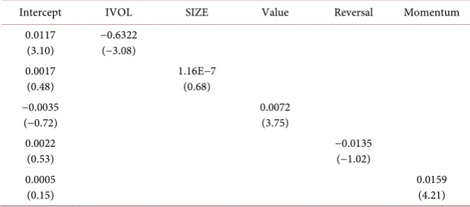
Table 6. Univariate Fama-Macbeth regression results. We perform firm-level

Fa-ma-MacBeth cross-sectional regressions on the return on that month with values of the control variables in the previous month for the full sample period. The time-series aver-ages of the slope coefficients and their associated t-statistics are reported in the table. IVOL is the standard deviation of the residuals of the FF3-factor model computed using the past 22 trading daily returns data. SIZE is the firms’ capitalization at the end of month

t; Value is the firm’s book-to-market ratio six months prior, i.e. at the end of t-6. Mo-mentum represents the stock’s 11-month past return lagged one month by following Je-gadeesh and Titman [28], i.e. return from month t-12 to month t-2. REV in month t is short-term reversal defined as the return on the stock in month t-1, following Jegadeesh

[29] and Lehmann [30]. Newey-West T-statistics are reported in parenthesis. , 1 0, 1, , 2, , 3,Value, 4,Reversal, 5,Momentum,

i t t t i t t i t t i t t i t t i t

R + =β +β IV +β MV +β +β +β .

Intercept IVOL SIZE Value Reversal Momentum

0.0117

(3.10) −0.6322 (−3.08) 0.0017

(0.48) 1.16E−7 (0.68)

−0.0035

(−0.72) 0.0072 (3.75)

0.0022

(0.53) −0.0135 (−1.02)

0.0005

(0.15) 0.0159 (4.21)

show significant momentum and BM effects with previous winners and stocks with high BM exhibiting higher returns. However we find no size and short-term reversal effects. The absence of a size effect is consistent with Morel

(15)

[image:15.595.206.539.229.361.2]

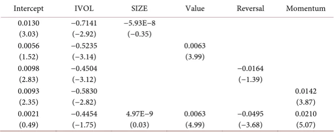
Table 7. Bivariate and multivariate Fama-Macbeth regression results. We perform a

firm-level Fama-MacBeth cross-sectional regression of the return on that month with values of the control variables in previous month for the full sample period. The time-series averages of the slope coefficients and their associated t-statistics are reported in the table. IVOL is the standard deviation of the residuals of the FF3-factor model computed using the past 22 trading daily returns data. SIZE is the firms’ capitalization at the end of month t; Value is the firm’s book-to-market ratio six months prior, i.e. at the end of t-6. Momentum represents the stock’s 11-month past return lagged one month by following Jegadeesh and Titman [28], i.e. return from month t-12 to month t-2. REV in month t is short-term reversal defined as the return on the stock in month t-1, following Jegadeesh [29] and Lehmann [30]. Newey-West T-statistics are reported in parenthesis.

, 1 0, 1, , 2, , 3,Value, 4,Reversal, 5,Momentum,

i t t t i t t i t t i t t i t t i t

R ₊ =β +β IV +β MV +β +β +β .

Intercept IVOL SIZE Value Reversal Momentum

0.0130

(3.03) −0.7141 (−2.92) −5.93E−8 (−0.35) 0.0056

(1.52) −0.5235 (−3.14) 0.0063 (3.99) 0.0098

(2.83) −0.4504 (−3.12) −0.0164 (−1.39)

0.0093

(2.35) −0.5830 (−2.82) 0.0142 (3.87)

0.0021

(0.49) −0.4454 (−1.75) 4.97E−9 (0.03) 0.0063 (4.99) −0.0495 (−3.68) 0.0210 (5.07)

Next we control the size, BM, reversal, and momentum effects individually with bi-variate Fama-MacBeth cross-sectional regressions and then simulta-neously in a multivariate regression. We report the results in Table 7. The biva-riate regressions show that none of our control variables can individually explain the negative IVOL effect. However if we control for all four variables simulta-neously, the IVOL coefficient becomes insignificant! Therefore, firm-level cross-sectional regression results indicate that the apparent negative IVOL effect in the French stock market is not robust and can be explained by our control va-riables.

4. Concluding Remarks

(16)

We find that both idiosyncratic and market volatility do not exhibit long-term trends. Instead their patterns are consistent with regime switching behavior sim-ilar to that in the U.S. and other developed countries. Though we initially find a negative IVOL effect in the French stock market which is robust in bi-variate Fama-MacBeth regressions, the negative IVOL effect promptly disappears when we control for these well-known effects simultaneously.

We add new evidence to the mounting results questioning the ubiquity of the IVOL effect which highlights the importance of country verification of so-called anomalies in the US, even in developed markets.

Acknowledgements

We thank two anonymous reviewers for their constructive comments. We also wish to thank the participants of the World Business, Finance, and Management Conference in December, 2014, Auckland, New Zealand for their comments and suggestions on earlier versions of this paper.

References

[1] Ang, A., Hodrick, R.J., Xing, Y. and Zhang, X. (2006) The Cross-Section of Volatil-ity and Expected Returns. Journal of Finance, 61, 259-299.

https://doi.org/10.1111/j.1540-6261.2006.00836.x

[2] Levy, H. (1978) Equilibrium in an Imperfect Market: A Constraint on the Number of Securities in a Portfolio. American Economic Review, 68, 643-658.

[3] Merton, R. (1987) A Simple Model of Capital Market Equilibrium with Incomplete Information. Journal of Finance, 42, 483-510.

https://doi.org/10.1111/j.1540-6261.1987.tb04565.x

[4] Ang, A., Hodrick, R.J., Xing, Y. and Zhang, X. (2009) High Idiosyncratic Volatility and Low Returns: International and Further U.S. Evidence. Journal of Financial Economics, 91, 1-23. https://doi.org/10.1016/j.jfineco.2007.12.005

[5] Bali, T.G. and Cakici, N. (2008) Idiosyncratic Volatility and the Cross-Section of Expected Returns. Journal of Financial and Quantitative Analysis, 43, 29-58.

https://doi.org/10.1017/S002210900000274X

[6] Bali, T.G., Cakici, N. and Levy, H. (2008) A Model-Independent Measure of Aggre-gate Idiosyncratic Risk. Journal of Empirical Finance, 15, 878-896.

https://doi.org/10.1016/j.jempfin.2008.02.002

[7] Huang, W., Liu, Q., Rhee, S.G. and Zhang, L. (2010) Return Reversal, Idiosyncratic Risk, and Expected Returns. Review of Financial Studies, 23, 147-168.

https://doi.org/10.1093/rfs/hhp015

[8] Malkiel, B. and Xu, Y. (2004) Idiosyncratic Risk and Security Returns. Paper Pre-sented in AFA 2001 New Orleans Meetings.

[9] Spiegel, M. and Wang, X. (2006) Cross-Sectional Variation in Stock Returns: Li-quidity and Idiosyncratic Risk. Working Paper, Yale University.

[10] Divatopolous, D., Doran, J. and Peterson, P. (2008) The Information Content in Implied Idiosyncratic Volatility and the Cross-Section of Stock Returns: Evidence from the Options Markets. Journal of Futures Markets, 28, 1013-1116.

https://doi.org/10.1002/fut.20327

(17)

of Financial Economics, 91, 24-37.https://doi.org/10.1016/j.jfineco.2008.02.003

[12] Chua, C.T., Goh, J. and Zhang, Z. (2010) Expected Volatility, Unexpected Volatility, and the Cross-Section of Stock Returns. Journal of Financial Research, 33, 103-123.

https://doi.org/10.1111/j.1475-6803.2010.01264.x

[13] Wei, S.X. and Zhang, C. (2006) Idiosyncratic Risk Does Not Matter: A Re-Examination of the Relationship between Average Returns and Average Volatil-ities. Journal of Banking and Finance, 29, 603-621.

https://doi.org/10.1016/S0378-4266(04)00050-0

[14] Fink, J., Fink, K.W., Grullon, G. and Weston, J.P. (2010) What Drove the Increase in Idiosyncratic Volatility during the Internet Boom? Journal of Financial and Quantitative Analysis, 45, 1273-1279.https://doi.org/10.1017/S0022109010000487

[15] Pukthuanthong-Le, K. and Visaltanachoti, N. (2009) Idiosyncratic Volatility and Stock Returns: A Cross Country Analysis. Applied Financial Economics, 19,

1269-1281.https://doi.org/10.1080/09603100802534297

[16] Suss, S. (2012) The Pricing of Idiosyncratic Risk: Evidence from the Implied Vola-tility Distribution. Financial Markets and Portfolio Management, 24, 247-267.

https://doi.org/10.1007/s11408-012-0183-4

[17] Liu, B., Di Iorio, A. and De Silva, A. (2016) Equity Fund Performance: Can Mo-mentum Be Explained by the Pricing of Idiosyncratic Volatility? Studies in Eco-nomics and Finance, 33, 359-376. https://doi.org/10.1108/SEF-04-2016-0081

[18] Aboulamer, A. and Kryzanowski, L. (2016) Are Idiosyncratic Volatility and MAX Priced in the Canadian Market? Journal of Empirical Finance, 37, 20-36.

https://doi.org/10.1016/j.jempfin.2016.02.005

[19] Gu, M., Kang, W. and Xu, B. (2018) Limits of Arbitrage and Idiosyncratic Volatility: Evidence from China Stock Market. Journal of Banking and Finance, 86, 240-258. [20] Campbell, J.Y., Lettau, M., Malkiel, B.G. and Xu, Y. (2001) Have Individual Stocks

Become More Volatile? An Empirical Exploration of Idiosyncratic Risk. Journal of Finance, 56, 1-43.https://doi.org/10.1111/0022-1082.00318

[21] Brandt, M.W., Brav, A., Graham, J. and Kumar, A. (2010) The Idiosyncratic Vola-tility Puzzle: Time Trend or Speculative Episodes? Review of Financial Studies, 23, 863-899.https://doi.org/10.1093/rfs/hhp087

[22] Bekaert, G., Hodrick, R. and Zhang, X. (2012) Aggregate Idiosyncratic Volatility.

Journal of Financial and Quantitative Analysis, 47, 1155-1185.

https://doi.org/10.1017/S0022109012000543

[23] Wikipedia (2017) Euronext. https://en.wikipedia.org/wiki/Euronext [24] Euronext (2017) We Are Euronext. https://www.euronext.com/event

[25] Bunzel, H. and Vogelsang, T. (2005) Powerful Trend Function Tests That Are Ro-bust to Strong Serial Correlation, with an Application to the Prebisch-Singer Hy-pothesis. Journal of Business and Economic Statistics, 24, 381-394.

https://doi.org/10.1198/073500104000000631

[26] Fama, E. and French, K. (1993) Common Risk Factors in the Returns on Stocks and Bonds. Journal of Financial Economics, 33, 3-53.

https://doi.org/10.1016/0304-405X(93)90023-5

[27] Fama, E. and French, K. (1996) Multifactor Explanations of Asset-Pricing Anoma-lies. Journal of Finance, 51, 55-84.

https://doi.org/10.1111/j.1540-6261.1996.tb05202.x

(18)

DOI: 10.4236/tel.2018.81005 96 Theoretical Economics Letters https://doi.org/10.1111/j.1540-6261.1993.tb04702.x

[29] Jegadeesh, N. (1990) Evidence of Predictable Behaviour of Security Returns. Journal of Finance, 45, 881-898.https://doi.org/10.1111/j.1540-6261.1990.tb05110.x

[30] Lehmann, B. (1990) Fads, Martingales, and Market Efficiency. Quarterly Journal of Economics, 105, 1-28.https://doi.org/10.2307/2937816

[31] Kong, G.W. and Kong, D.M. (2015) Institutional Investors’ Trading in Speculation: Evidence from China. South African Journal of Economics, 83, 617-631.

https://doi.org/10.1111/saje.12073

[32] Dickey, D. and Fuller, W. (1979) Distribution of the Estimator for Autoregressive Time Series with a Unit Root. Journal of the American Statistical Association, 74, 427-431.

[33] Duncan, A. and Kabundi, A. (2014) Global Financial Crisis and Time-Varying Volatility Movement in World Equity Markets.South African Journal of Economics,

82, 531-550.https://doi.org/10.1111/saje.12033

[34] Vogelsang, T. (1998) Trend Function Hypothesis Testing in the Presence of Serial Correlation. Econometrica, 66, 603-621.https://doi.org/10.2307/2998543

[35] Nartea, G.V., Wu, J. and Liu, Z.T. (2013) Does Idiosyncratic Volatility Matter in Emerging Markets? Evidence from China. Journal of International Financial Mar-kets, Institutions and Money, 27, 137-160.

https://doi.org/10.1016/j.intfin.2013.09.002

[36] Stotz, O., Wanzenried, G. and Dohnert, K. (2010) Do Fundamental Indexes Pro-duce Higher Risk-Adjusted Returns than Market Cap Indexes? Evidence for Euro-pean Stock Markets. Financial Markets and Portfolio Management, 24, 219-243.

https://doi.org/10.1007/s11408-010-0135-9

[37] Brockman, P. and Yan, X. (2006) The Time-Series Behavior and Pricing of Idiosyn-cratic Volatility: Evidence from 1926-1962. Working Paper, University of Missouri. [38] Drew, M., Malin, M., Naughton, T. and Veeraraghavan, M. (2006) Idiosyncratic

Volatility and Security Returns: Evidence from Germany and United Kingdom.

Studies in Economics and Finance, 23, 80-93.

https://doi.org/10.1016/j.intfin.2013.09.002

[39] Newey, W.K. and West, K.D. (1987) A Simple, Positive Semi-Definite, Heterosce-dasticity and Autocorrelation Consistent Covariance Matrix. Econometrica, 55, 703-708.https://doi.org/10.2307/1913610

[40] Morel, C. (2001) Stock Selection Using a Multi-Factor Model—Empirical Evidence from the French Stock Market. European Journal of Finance, 7, 312-334.

https://doi.org/10.1080/13518470110071137

(19)