ON THE NUMERICAL SOLUTION OF A
FUNCTIONAL DIFFERENTIAL EQUATION
PERTAINING TO A WAVE EQUATION
by
David J.N. Wall
Department of Mathematics, University of Canterbury, Christchurch, New Zealand.
No. 57 October, 1990.
Abstract
The numerical solution of the invariant imbedding equation, describing time domain, one dimensional direct scattering from a slab in which the material properties are spatially varying, is considered. It is proven that the equation discretised by the Trapezoidal rule has an asymptotic expansion for the global error involving only even powers of h. This expansion is utilised to generate a high order integration method by use of polynomial extrapolation. The method is suitable for adaptation to parallel computation, and by virtue of this together with its higher order integration, it constitutes a fast algorithm when compared with the current methods of solution of this equation.
AMS(MOS) classifications: 78A45, 65L05, 65R20.
David J. N. Wall
Dedicated to the memory of Bob Krttegcr
Abstract. The numerical solution of the invnrinnt imbedding equation, describing time domain, one dimensional direct scattering from a slab in which the material properties are spatially varying, is considered. It is proven that the equation discretised by the Trapezoidal rule hns an asymptotic expansion for the global error involving only even powers of h. This expansion is utilised to generate a high order integration method by use of polynomial extrapolation. The method is suil.nble for ndaptntion l.o parallel comput.nt.ion, nnd by virtue of this toget.her with its higher order integrntion, it. constitutes a fll.'lt nlgorithm when compared with the current methods of solution of this equation.
1. Introduction. The use of a reflection kernel to characterise the scattering of waves in an inhomogeneous medium in the time domain, has been well developed over the last ten years (see for example [4] - [11] and the references cited therein). In [4] it is shown that the use of a reflection kernel combined with invariant imbed-ding provides a useful and convenient method for the computational solution of a. varict.y of inverse problems. In particular this technique leads to explieit functional equations for the mapping between the reflection kernel, measured at the interface of the inhomogeneous region, and the material functions to be identified. In all previous papers utilising this technique the numerical algorithm used has been the implicit Trapezoidal rule. While this method has provided excellent results it suffers from two major defects in its implementation.
(i) A low order of approximation of the operator equation. (ii) No error est.imat.ion.
Our algorithm while still being based on the Trapezoidal rule overcomes both of these problems. In this paper we shall examine an efficient computational method
2
David J .N. Wall : Solution of a Functional Differential Equationfor solution of the direct problem of determination of the reflection kernel, at the interface, when the properties of the inhomogeneous medium are known. Once this kernel is known the reflected wave can be calculated by a convolution.
The method used to solve the problem converts the problem to a functional differential equation which is then solved by the Trapezoidal rule and a global extrapolation technique based on the asymptotic expansion of the global error. This method has several computational advantages not the least of which is that the algorithm is readily adapted to parallel computation. However we should point out the extent to which the algorithm can be parallelised cannot exceed the depth of the extrapolation table (see §3). For a recent review on extrapolation methods see (13]. We shall require several of our results proven in (17] in the sequel.
In the §2 the relevant equations are discussed and it is shown that the prob-lem for determination of the reflection kernel can be reduced to the solution of a functional differential equation. The appropriate properties of the solution of this equation are then displayed. In §4 it is shown that the asymptotic expansion of the solution, obtained via the numerical method described in §3, has even powers of the step size parameter. This enables high order polynomial extrapolation methods to be utilised in the integration of the differential equation. The reflection kernel can be efficiently found when the extrapolation integrator is combined with an adaptive cubic spline interpolation procedure. §5 provides some numerical evaluation of our algorithm.
2. Preliminaries. The one-dimensional spatial wave equation modelling wave motion in the z-direction within a slab, to be investigated in this paper, is
Uzz- c(z)-2Urr
+
a(z)Ur+
((z)Uz = 0, (2.1)where c(z) is the wave speed of the medium, a(z) is the damping (attenuation) parameter, and ( is given parameter, again ( = ((z). The dependent variable U
is dependent upon z and the temporal variable r and is independent of x, y. The
region of interest is a
<
z< b
and as our concern is with the impulse response of the medium we assume a, (are zero outside the interval (a, b] and c(z) = c(a) forz
<
a andc(
z)=
c(
b) for z>
b. It is convenient to make the change of coordinatesx(z)
=
lz
c(s)-1 ds/C,t
=r/C,
C
=
1b
c-1(s) ds,u(x,
t)
=U(z, r ),where the independent variable x is a travel time coordinate. Equation (2.1) now becomes
where
Uxx- Utt
+
A(x )ux+
B(x )ut=
0,A(x)
= _
d ln c(z)+
d(,dx
B(x) = -c2£a.
(2.2)
permittivity, the magnetic field equation is of the form (2.1) and then travel time conversion takes it to (2.2) with exactly the same form as the equation obtained via the derivation through the electric field equation (as is done for example in (4]).
Equation (2.1) is sufficiently general to model a variety of electromagnetic and elastic wave scattering phenomena and we shall only consider its normalised version (2.2) in the sequel. The coefficients A and B are thus related to the material parameters and as such B ~ 0, with B related to dissipation (energy loss) within the slab. The results presented in this paper however do not require the coefficients to have one sign. The coefficients are to have support on the interval x E [0, 1), and are assumed to be continuous. For simplicity in the sequel, as previously stated, we shall assume the slab is matched to the homogeneous exterior region; this will mean
A(x)
=
0, B(x)=
0,A(x) = 0, B(x) = 0,
X<
0,x>l.
This requires that in the physical problem the wave speed is continuous in ( -oo, oo ). Means of overcoming this restriction are considered in [10).
In [6) Corones and Krueger utilise the technique of invariant imbedding to derive from (2.2) the integra-partial differential equation
Rt(x, 1; t)- 2Rt(x, 1; t)
=
_!(A(x)+
B(x))t
R+(x, 1; s)R+(x, 1; t- s) ds2
Jo
- B(x)R+(x,1;t), 0 ~ x ~ 1, 0 ~
t
~ 2(1- x). (2.3) This is the imbedding equation describing the reflection kernel at the left-hand interface at location x with the right-hand interface held at x = 1. The superscript+
is used to signify that this kernel transforms an incident wave moving in the positive x-direction from the left-hand-side of the medium into a reflected wave moving in the negative x-direction. A similar equation holds for the reflection kernel at the right-hand interface, namely R-(O, x, t), describing the reflection, at location x, of an incident wave from the right-hand medium with the left-hand interface held at x = 0. The equation satisfied by R- can be obtained from (2.3) if the functional dependence on x is replaced by 1- x,Ri;
is then replaced by-R;,
and the A term is multiplied by -1 since A involves a derivative with respect to x(see [9) for further details).
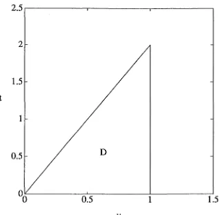
We define the triangular region in the independent variables (
t,
x) for which (2.3) is applicable as D = {(x,t)
E ffi2: 0 ~ X ~ 1, 0 ~
t
~ 2(1 -X)}. When theproblem is one of direct scattering the material functions A(x), B(x), x E [0, 1), are known and hence
1
R+(x, 1; 0) =
-4
(A(x)- B(x)), 0 ~ x ~ 1,(2.4)
on the side of D where
t
= 0, and it is required to calculate the reflection kernelR+(o, 1; t),
o
~t
~ 2,(2.5)
4 David J .N. Wall : Solution of a Functional Differential Equation
2 . 5 . - - - . . . - - - . - - - ,
2
1.5 t
1
0.5 D
0.5 1 1.5
[image:5.597.126.445.99.410.2]y
Figure 1. Illustrating the domain of definition of (2.6); the domain for a single return trip is D.
is of interest, and we shall consider this more general setting in a later paper. It should also be noted that the directional derivative on the left-hand side of (2.3) will complicate the direct numerical solution of this equation.
We shall now consider the computational method applied to the solution of the direct scattering problem associated with (2.2) and (2.3). It is essential for the computational scheme by which we solve the problem to convert (2.3) to a functional differential equation. To this end we. shall consider the change of independent variable y = x
+
t/2 in order to convert the partial derivatives on the left-hand side of (2.3) into a directional derivative. This will transform the region D into 0 :::; y :::; 1, 0 :::; t :::; 2y, see Figure 1.On redefining the dependent variable as u(t; y)
=
-2R(y- t/2, t)=
-2R(x, t) we finddu 1 {'
dt
=
-B(A(y-t/2)+
B(y- t/2))Jo
u(s;. y)u(t- s; y) ds1
+
2B(y- t/2)u(t;y), 0:::; t:::; 2y, 0:::; y:::; 1,(2.6)
with initial conditions 1
The direct scattering problem can now be stated as: given u(O;
y),
for 0 :::;y :::;
1, find u(t;t/2), for 0:::; t:::; 2, (or equivalently u(2y;y), for 0:::; y:::; 1) from the solution of the Volterra functional differential equation (2.6).In order to consider the theoretical aspects of the solution of (2.6) we find it convenient to consider equations (2.6), (2. 7) through B-space ordinary differential equation theory. Y.,Te theref~re rewrite (2.6) in the standard form
du
dt(t; y)- f(t, u(t))(y)
=
0, 0:::; t :::; 2, (2.8)with initial conditions
u(O) - uo
=
0, and where uo=
u(O; y), 0 :::; y :::; 1, (2.9)where u0 , u E Y and Y is the B-space of continuous functions C([O, 1]) with norm
llullv
=
sup { u(t; y)},YE[0,1)
for fixed t E [0, 2]. This will mean for fixed t the function u(t)
=
u(t; y)=
-2R(x,
t)will form points of the B-space Y. The mapping function on the right-hand side of (2.8)
f :
[0, 2] x Y ~--+ Y is described by-k(A(y- t/2)
+
B(y- t/2))J;
u(s; y)u(t- s; y) ds+tB(y- t/2)u(t; y), 0:::; t:::; 2y;
f(t,u)(y)=
-k
(A(O)+
B(O)) fot u(s; y)u(t- s; y) ds+tB(O)u(t; y), 2y:::;
t:::;
2.(2.10)
Noticef
is defined to be continuous att
= 2y. We set U to be the space of continuous functions u : [0 :::; t :::; 2] H Y, that is U = C([O :::; t :::; 2], Y) and thenorm for U is
llullu
=
sup llu!!v, (2.11)o::;t:=;t
then (U,
II·
llu) is a B-space. We shall also assume that A, B belong to the parameter subspace P, P = C([O, 1]) which is a B-space with the appropriate supremum norm. Thus (2.8) describes a system with memory in the t variable, but not in the yvariable. This later property will mean (2.8) is particularly efficient for computation. Equation (2.8) is a functional differential equation for u but it cannot be put into the standard form for a Volterra integra-differential equation because of this memory; it is in fact a Volterra functional differential equation.
We define Ua to be the space of continuous functions Ua = C([O:::;
t:::;
a],
Y),0 :::; a :::; 2, with an appropriate norm modelled on (2.11). To proceed further we need the regularity properties of
f.
LEMMA 2.1. With
f
defined a.'J in (2.10) and with A, B E P then the mappingf
ha.'J the following propertie.'J.6 David J .N. Wall : Solution of a Functional Differential Equation
{ii) For each u E Y, f(t, u) is continuous with respect tot.
{iii) For each t E [0, 2] andy E [0, 1], f is Frechet partial differentiable with respect to u and with f u
=
~(
t, u) : T H T this derivative is defined by the differential(fu(t,u)v)(y) =
~B(y- t/2)v(t; y)- HA(y- t/2) +B(y- t/2))
J;
u(t- s; y)v(s; y) ds,~B(O)v(t; y)
0 :::;
t :::;
2yj-t(A(O)
+
B(O))
J;
u(t-s; y)v(s;
y) ds, 2y:::;t:::;
2. (2.12) (iv) For each t E [0, a], 0<
a :::; 2 and y E [0, 1], f is Lipschitz continuous with respect to u in the ball BM = {u E Ua: llullu" :::; M}, with Lipschitz constant equal to ~IIBIIP+
HIIAIIP
+
IIBIIP
)M.(v) For each t
E [0, 2]
andyE [0, 1],
f is continuous with respect to A and B. {vi) For each tE [0, 2]
andyE [0, 1],
f is Frechet partial differentiable with respectto A or B.
(vii) if(x, u)l:::; ~IIBIIPIIuiiY(t)
+
k(IIA +Blip)
J;
llully(s)llully(t-
s) ds, where the notationlluiiY(s)
is used to explicitly illustrate that the scalar quantity llully is a function of the time like variable s.(viii) For each t E [0, 2) and y E [0, 1], f is infinitely Frechet partial differentiable with respect to u, with
i(A(y- t/2
+
B(y- t/2))-(fuu(x,u)vw)(y) = x
J;
v(t- s; y)w(s; y) ds,0:::;
t:::; 2y; (2.13)t{A(O)
+
B(O)),
2y:::;t:::;
2,and with all derivatives after this one being the zero operator.
(ix) For each t E [0, a], 0
< a :::;
2 andy E [0, 1], fu and fuu are Lipschitz continu-ous, the former with respect to u in the ball B M, as given in item {iv ), and the latter for all Ua. Note that the second derivative off is a scaled convolution operator. Proof. Items (i) - (vii) are proven in [17] and (viii), and (ix) follow by straight forward analysis, see [17].With this result it then follows that (2.8) has only one solution [17].
THEOREM 2.1. With uo E Y, A,B E P, and f possessing the properties of Lemma 2.1 the direct scattering problem (2.8) has exactly one continuously differ-entiable solution u E U for all t E [0, 2]. The solution depends continuously on the initial data
(2. 7)
and the parameters A and B.COROLLARY 2.1. With PC C(m)([O, 1]) and the conditions of Theorem 2.1
holding, (2.8) has exactly one (m
+
1)th continuously differentiable solution u E U for all t E [0, 2). The solution depends continuously on the initial data (2. 7) and the parameters A and B.Proof. This follows from Lemma 2.1(vi).
numerical scheme we use to solve (2.8) is the implicit Trapezoidal method with the numerical quadrature required in (2.10) also being performed by this method. A uniform step size, h, is chosen with global extrapolation being used to obtain a high order method. This uniform step size and the discretisation method chosen has the important computational advantage that u(t) for past values oft, 0
S
tS
2, is available for use in the quadrature rule, for the lag termit
u(s; y)u(t- s; y) ds,without the necessity of using polynomial interpolation.
The implicitness of the Trapezoidal rule poses no difficulty for (2.8) as by the nature of the non-linearity of u in the integral in (2.10) the resultant algebraic equation for u(
t
+ h)
can be solved explicitly. The implicit Trapezoidal method is A-stable, and global extrapolation of this method does not affect this result. However note that if local extrapolation were to be used the higher order methods obtained in the extrapolation table would only be A( a) stable; see for example [16, chapter 6].We now discuss the numerical difficulties which might be encountered in inte-grating (2.8). The measure of stiffness of (2.8) is
lful
<a+
2(3C,where
a= tiiBIIp,
(3=
~(IIA+Blip),
andC = exp(2a)~I1(4~),
with
h
the modified Bessel function of the first kind andwo
=
lluoi!Y S
!(IIAIIvl
+
IIBIIv)·
This follows from Lemma 2.1(iii), (vii) and the comparison equation utilised in the proof of Theorem 2.1 [17]. Typical values of A and B for a particular ap-plication are difficult to predict. The possibility of (2.8) being stiff exists for the normal range of parameters is highly problem dependent, for exampleIBI
can be of the order of 106 • One of the major problems associated with the Trapezoidal rule is that although the method is A-stable, and therefore numerical instability is not a problem, it is not L-stable [14, Chapter 8]. This will mean the method will not provide an accurate solution unless the initial transient response is integrated accu-rately, that is with small h values. However as the initial transient is all important in inverse problems one presumes that this transient will be calculated accurately. Then the error in this rapidly decaying term will be small and the Trapezoidal method will yield an accurate answer with moderate values of h for the rest of the integration.The integral term in (2.10) is of convolutional form and straight-forward eval-uation of this integral at
t,
where h = tjn, will have a computational cost of O(n2 )8 David J .N. Wall : Solution of a Functional Differential Equation
equation the kernel in the integral is known for all values of the independent vari-able, whereas this is not the case in (2.8). A moment's reflection shows that this FFT 'trick' is not possible for a convolution Riccati equation such as (2.8). However the symmetry of the quadratic integrand in the integral operator in (2.10) and in its Trapezoidal summation, namely
t
nJo u(t- s)u(s)ds
=
h L:"ujUn-j,0 j=O
h
=
tjn,
(3.1)indicates that the computational cost can be halved to 0( n2 /2). In (3.1) the double
prime on the summation signifies that the first and last term are to be halved. 3.1 Global Error Estimation of the solution. Consider the discrete method just discussed and denote its numerical solution by u(t, h)
=
Un, to ex-plicitly show its dependence on step-size. Then it is shown in Theorem 4.1 that the global error has an asymptotic expansion of the formwith the { ej H~
1
being independent of h. If the numerical solution at t when computed for the different step sizes h, h/2, h/4, ... is denoted by Ti,o=
u(t, h/2i), then the extrapolation tableauTo,o
T1,0 T1,1 T2,o T2,1 T2,2
can be calculated according to the Neville-Aitken algorithm
'D .
=
'D . Ti,k-1 - Ti-1,k-1a,k a,k-1
+
4k _ 1 i~k~l.
This algorithm cancels the leading term in the asymptotic expansion of Ti,k-1 so that the global error of Ti,k is O(h2k+ 2), that is
Thus by building up the tableau, if we are prepared to solve the problem for i
+
1 step sizes we can generate an estimate for u(t) that is at least asymptotically O(h2i+2 )accurate.
We now discuss the convergence test. Define the row difference dr(i, k)
=
T(i, k)- T(i, k- 1),then for a prescribed tolerance tol the extrapolation tableau is calculated until row convergence in two successive rows is obtained; that is
and
ldr(i, k)j
:S
tol X jT(i, k)j.By these considerations the dr estimate the relative error of Ti,k! and then the more
accurate value Ti,k is to be accepted as a numerical approximation to u(t).
If a column difference ·
dc(i, k) = T(i, k)- T(i- 1, k),
is defined we observe from (3.2)
(i k- 1) = dc(i- 1' k- 1) 4k J{
>
1, as i t'ncreases.r ' dc(i,k-1) --+ ' (3.3)
Consequently this ratio can be checked numerically. However this number will lose significance rapidly on a finite precision machine.
We again note this algorithm lends itself readily to parallel computation in that (2.8) can be simultaneously integrated out to 2y for different step sizes and then global extrapolation carried out.
3.2 Adaptive Interpolation. It remains to describe how the remainder of the problem is solved. The differential equation must be integrated to 0 :::;
t :::;
2y, for all 0:::; y:::; 1, to obtain u(2y, y). This is achieved with minimum cost by use of an adaptive interpolation algorithm which will minimise the number of points y at which (2.8) will have to be integrated. We will interpolate u(2y, y) for 0 :::; y :::; 1 by a cubic spline. In order to provide a foundation for the adaptive algorithm it is necessary to estimate the error bound between the cubic interpolatory spline andu(2y, y). This will ensure that a suitable sub-division of y E [0, 1] is made which is dependent upon the magnitude of the fourth derivative of u(2y, y). A decision as to which interpolatory cubic spline is to be used must be made with possible candidates being from the 'derivative free' class. Therefore possible candidates would be the
not-a-knot or the clamped spline obtained by forcing the end derivatives of the spline to agree with that of a local cubic interpolant. The error for these cubic 'derivative free' interpolating splines on the mesh [0
=
Yo, Yl, · · · , Yn=
1] is given by [1]les(Y)I
=
IS(y)- u(y)l:::; u<4)(2e,e)h'!naxCs, e E (0, 1), (3.4)10 David J .N. Wall : Solution of a Functional Differential Equation
fitted to the first four nodes formed when the interval size is now h/2. The accuracy test is then repeated and the process continued until the accuracy test is achieved. The algorithm thereby marches towards the node y
=
1 so ensuring each local cubic interpolation polynomial on each successive four nodes of the resultant mesh has an error less than e L. Recall that tpe error between the local cubic interpolationpolynomial and u, with a uniform spacing h, is given by
where Ca
=
1/16. The error when using the cubic spline on this interval is given by (3.4), but with hmax = h. Then if we require the global error for the interpolatory spline to be less than tol, a prescribed tolerance, that islesl
<
tol, it is seen that when using the local cubic strategy we must ensure that the error incurred by this polynomial isThe error tolerance for the spline fit will then be satisfied. Observe that although this is only a local result the global error is also bounded by tol.
It should be noted that other adaptive approximation algorithms for cubic spline interpolation have been suggested [15, §21.3], [8, Chapters XII and XI]. How-ever these references solve this fully non-linear problem by iterative techniques and do not use the local cubic approximation ideas incorporated here.
4. Asymptotic Error Expansion of the Discretisation Method. Prior to proving the main theorem in this section we shall define our terminology. By following the notation of [16] it is convenient to define the Banach spaces,
with norm in Eo
E = C(1
)([0
S
t
s
2], Y),Eo
=
Y x C([OS
t
S
2], Y),11
w(:lr~)
t.
=llwollv
+
llw(t)llu.
Observe that the superscript 1 on C(l) denotes that it is the space of continuously differentiable functions with respect to
t.
For this section we define the operator Fto stand for (2.8) and (2.9), so that
Fu- [ (u(O)-uo)(y)
l
EEo, E- u(l)(t;
y)-
f(t, u(t))(y) u E 'with the notation that u(l) denotes the derivative du/dt. The discretisation ofF is
associated with the finite dimensional Banach spaces En, Eg for the discretisation parameter n. Note these spaces are different for each value of n. We assume n is chosen from a set JN' C lN, lN denoting the natural numbers. The discretised operator is denoted by Fn with Fn :En H Eg, and appropriate restriction operators
to simply quote Stetter's [16, Theorem 1.3.1] and then to show that our problem satisfies all the conditions required to complete this. However his theorem requires several technical definitions and for our problem it is simpler, and more transparent, to prove the result directly. First recall the definition of the consistency error map. DEFINITION 4.1. The sequence of mappings, dependent upon n, An : E H
Eo, n E JN', such that
Fnrnw = rg[F
+
An]w, for all w in the domain ofF, is called the consistency error map.Remark 4.1. The consistency error Cn
=
Fnrnw- r?tFw is generally defined for n -+ oo, whereas Definition 4.1 is taken to apply for all n E JN'.The commutativity diagram illustrates the relationship between the various spaces and definitions.
With En, Un, and u denoting the global error, the exact solution of the
dis-cretised problem and the exact solution of the continuous problem respectively, the definition of the global error implies that these terms are related through
( 4.1) So applying the operator Fn to ( 4.1) it follows
(4.2)
To find a general expression for the global error observe from ( 4.1)
as FnUn
=
0 and furtherwhere Cn is the consistency error of the discretised problem to the continuous one. Therefore if
F;;
1 satisfies a Lipschitz condition uniformly in n then(4.3)
12 David J.N. Wall: Solution of a Functional Differential Equation
If
J J
F(w
+I:
hiej)+
An(w+
L
hiej) = O(hJ+I ), ash - t 0, (4.4)j=l j=l
where the ej are to be defined, then Definition 4.1 shows
J
Fn(rn(w
+
L hiej))=
O(hJ+l ). j=lEquations ( 4.2) and ( 4.4) then imply we have an asymptotic expansion of the global error
J
€n
=
rn[Lhiej]+
O(hJ+l) ash - t 0, (4.5)j=l
where ej are now the elements of the asymptotic global discretisation error. In ( 4.5) if the discretisation scheme is convergent of order p then the ej
=
O, 1S
jS
p- 1, and also if the global discretisation contains only even powers of h, then e(2j-l)=
0, 1S
jS [
J /2]. We may now state the central result of this section.THEOREM 4.1. The discretisation of (2.8) by the Trapezoidal rule implies that the :wlution of the discretised equation will possess a unique asymptotic expan-sion to order 21 of the form
J
€n = rn(L h2ie2j)
+
O(h2J+2)j=l
provided the conditions of Theorem 2.1 and Corollary 2.1, with m
=
2J+
1, are satisfied.Proof. It is obvious from the definition ofF, and its discretisation, that the first component of An is zero. The second component of the consistency error mapping is given by
w(t + h/2)
~
w(t- h/2) -~[f(t
+ h/2, w(t + h/2)) + f(t- h/2, w(t- h/2))] - w'(t)- f(t, w(t)), w E E,(4.6) for notational simplicity we have not explicitly written the Trapezoidal quadrature rule within the square brackets, but the understanding is that each integral term within this bracket is to be replaced by its Trapezoidal approximation, see (3.1). Use of Taylor's formula and the Euler- MacLaurin formula in ( 4.6) then verifies for each positive integer J, the An, n E 1N', possesses an asymptotic expansion to order 2J and its second component is
J
" ' [ 1 (2i+l) ( ) 1 (2j) ( ( ))
~ (2j+ 1)!Dt wt -(2j)!Dt jt,wt
J -21 ( )
B2j " ' h 21 (21) d 21-1
I ]
h 2. + (2j)!(£-i'(2) Dt {g(t)ds(21-l)(w(t-s)w(s))} s=t (2) J,where g(t) = -~(A(y- t/2)
+
B(y- t/2)) and the B2j denote the even Bernoullinumbers. The smoothness assumption on w to achieve ( 4. 7) is that w E C2J+3(0
s:;
t
s:;
2). We note if u E C2'+
3(0s:;
ts:;
2) equation (4.7) is the consistency error ofthe problem. It should be observed that in general unless the solution is smooth enough, the actual consiste1,1cy error obtained, and the consistency error mapping need not be the same. Equation (
4. 7)
can also be writtenJ
llrg[Anw-
L
h2i-\2jwJiiE~ = O(h2J+2), ash --t 0, (4.8)j=1
where the operators A2j (which are independent of h) are given by the coefficient of h2i in ( 4. 7). Notice that the first component of this mapping which is associated with the initial condition is just the zero operator. The asymptotic expansion for the global error is expected to contain only even powers of h because of ( 4. 7).
Throughout the remainder of the proof the superscript ( k) appended to operators will denote the Frechet derivatives of the operators with respect to the variable w. It is important for the sequel to note that the implicit 'frapezoidal method introduced in §3 is stable, that is
F;;
1 satisfies a Lipschitz condition, compare with ( 4.3), and also (F<l)( w ))-1 exists.The proof can now proceed by showing that (4.4) holds when w
=
u, and u is the solution of Fu=
0. To do this the mappings F and An are expanded by Taylor series. First observe that:(i) The -\2j are non-linear operators because of the second term in ( 4. 7) and
-XW
is given by A2j, but the second term involving f is replaced by fw, also(2) [ 0 ]
-\2. 1 = -1 (2j) 2 '
(2j)!Dt fww(t,w(t))e (t)
d dm)
an A2j = 0, m
>
2.(ii) The Frechet derivatives of F are
F(1)( ) _ [ e(O) ]
w e - e'(t)- fw(t, w(t))e(t) '
F(2)(w)e2
=
[fww(t,~(t))e2(t)]'
with the linear operators fw and fww given by Lemma 2.1, and with e1 denoting dejdt.
Now F( w
+
L:,f=l
h2ie2j) +An( w+
L:,f=1
h2ie2j) expands to(
J ) J J
(J-j
)
F(w)
+
p(l)(w)t;
h2ie2j+
t;
h2i-\2jw+
t;
h
2i-\~Y(w)
t;
h2ke2k]+
~!
[F<2)( w)
+
,\~~)(
w )]((t
h2ie2j )2)+
R2J( w; e2, e4, · • ·, e2J ),)=1
14
1.5
1
0.5
0 0
David J .N. Wall : Solution of a Functional Differential Equation
(a)
1.5 xJ0-3 (b)
1
[image:15.595.93.498.93.248.2]0.5
...
0
0.5 1 0.4
lA
.J\J
0.6 0.8
X X
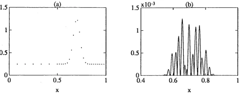
Figure 2. An example illustrating the distribution of nodes (a) and the pointwise absolute error (b) obtained from the adaptive in-terpolation algorithm when fitting a 'bell-shaped' function 0.25
+
exp[ -400( x-. 7)2]; the dots indicate the interpolation nodes necessary to attempt to achieve a global error tol
<
10-2.1
and when w
=
u the first term disappears and our previous assumptions ensureif the e2j, 1 ~ j ~ J are defined from
with
e2j(O)
=
0,e~j(t)- fu(t, u(t))e2j(t) = b2j, t E
[0, 2],
b2 = --\2u(t)
b4 = --\4u(t)- A2e2(t)-
~fuu(t, u)e~
b6
=
-A6u(t)- A4e4(t)- fuu(t, u)e2e4 etc.(4.10)
Observe the bj are the coefficients of h2i on the in ( 4.9). Note that with u E
0(21+ 3)([0 ~ t ~ 2], Y) and fu, fuu satisfying Lipschitz conditions (Lemma 2.1(viii)) it follows that the recursive definition of the e2j is well defined from ( 4.10). We observe that (4.10) have been obtained by equating like powers of h of the second and third of the terms in (4.9) to those of the fourth term. This ensures (4.10) reduces to 0( h2 1+2) and our result follows from ( 4.4) and ( 4.5 ).
Remark
4.
2. The result of Theorem 4.1 is only true if the implicit trapezoidal rule is solved exactly at each step; this will mean the implicitness is removed either analytically or by solving the equation by a recursive method to convergence. That this is possible for (2.8) is shown in §3.(a)
1.5 . - - - ' T ' - - - . , 1.5 xl0-3
0.5
0 0
1
0
-1 -2 -3 0
5
0
-5
-10 0
[image:16.605.95.495.112.270.2] [image:16.605.97.521.383.707.2]0.5
...
.,·...
0
0.5 1 0.4 0.6 0.8
X X
Figure 3. An example illustrating the distribution of nodes (a) and the pointwise absolute error (b) obtained from the adaptive in-terpolation algorithm when fitting a 'bell-shaped' function 0.25
+
exp[-lOOO(x- .7)2 ]; the dots indicate the interpolation nodes nee-essary to attempt to achieve a global error tol<
10-3 •0.2 0.4 0.6 0.8 1 1.2 1.4 1.6 1.8
A=30 B=-10
0.2 0.4 0.6 0.8 1 1.2 1.4 1.6 1.8
Figure 4. An example illustrating the distribution of nodes obtained from the adaptive integration algorithm when tol
=
10-4 and (a)A= 10, B = 0, (b) A= 30, B = -10.
1
2
16 David J .N. Wall : Solution of a Functional Differential Equation
T(i, 0) T(i, 1) T(i,2) T(i, 3) T(i, 4) 0 1.12209789152
1 1.02824308029 0.996958143217
2 1.00284087142 0' 994373468466 0.994201156816
3 0.996360203086 0.994199980307 0.994188414430 0.994188212170
4 0.994 731758755 0.994188943979 0.994188208223 0.994188204950 0.994188204922
r(i,O) r(i, 1) r(i,2)
1 3.7 2 3.9 3 4.0
14.9
15.7 61.8
Table 1. Extrapolation table for R(O, 0.5), when A = 10 and B = 0, and ratios of extrapolation columns. The exact solution for this case is R(O, .25)
=
0.99418820492855.( See exact solution in [17, equation 4.8]. Note there is a typographical error in this equation, the left-hand side should be divided by (2,8)).T(i, 0) T(i, 1) T(i, 2) T(i, 3) T(i,4)
0 0.461940032555
1 0.310108818451 0.259498413750
2 0.247628259314 0.22680140626 0.224621605770
3 0.231254187457 0.225796163504 0.225729147320 0.225746727344
4 0.227133359773 0.225759750545 0.225757323014 0.225757770247 0.225757813553
i
1 2 3
r{ i, 0) r{i, 1) 1'(i,2)
2.4
3.8 32.5
4.0 27.6 39.3
Table 2. Extrapolation table for R(O, 0.35), when A = 30 and B = -10, and ratios of extrapolation columns. The exact solution for this case R(O, 0.35) = 0.22575780953328. If the extrapolation is continued further it is found that T(6, 4) has converged to at least 12 significant decimal digits; these extra columns have not been shown for reasons of space.
[image:17.597.71.507.85.256.2] [image:17.597.63.513.95.460.2]accuracy than is actually rquired. Figures 4( a) and 4(b) show the result of using the full algorithm to solve (3.1) for the accuracies and with parameters specified in the figure caption. The nodes and function values to be utilised in the spline are illustrated by circles showing the coarser mesh which suffices when the fourth derivative of the reflection kernel is small. Note that when the spline is fitted through these values a smo~th 02 function shown by the full line is obtained.
Tables 1 and 2 show the extrapolation tableaux for the integration algorithm and they illustrate convergence, to seven significant decimal places, in the inte-gration rule with consistency errors O(hB) and O(h10 ), respectively. Listed below the T1s are the ratios for the respective tableaux. Observe for Table 1 the basic
Trapezoidal rule T( 4, 0) achieves 3 significant decimal digits of accuracy whereas the rules T(2, 2) and T( 4, 4) have 4 and 11 significant decimal digits of accuracy re-spectively. The Trapezoidal rule would require very many more intervals to achieve the accuracy of T( 4, 4). In Table 2 similar high accuracy results are obtained by the extrapolation integrator.
It should be observed that the numerical values in the ratio tables in many cases have not achieved the asymptotic value predicted by (3.3); this is because the ratios shown are only for low values of i.
6. Conclusions. Theorem 4.1 has provided a theoretical basis for a high order extrapolation algorithm that still provides all the advantages of the simple Trape-zoidal rule, namely convenient integration of the lag term coupled with stability properties. The transformation employed in §2 enables application of an efficient adaptive interpolation algorithm. Together these two algorithms provide efficient solution of the functional differential equation of §2. Although the transformation is not possible in problems involving multiple wave speeds it is possible to produce adaptive high-order integration algorithms for such problems, and this is being cur-rently investigated.
Acknowledgement.
I wish to thank my colleague Bob Broughton for discussions on the numerical solution of ordinary differential equations.
REFERENCES
[1 J R.K. Beatson, On convergence of cubic spline interpolation schemes, SIAM J. Numer. Anal., 23, (1986), pp. 903-912.
[2]
R.K. Beatson and E. Chacko, Which cubic spline should one use?, Depart-ment of Mathematics Preprint, University of Canterbury, Christchurch, New Zealand, 1990.[3] H.
Brunner and P.J. van der Houwen, The Numerical Solution of Volterra Equations, Elsevier Science, Amsterdam, 1986.[4] J.P. Corones, M.E. Davison and R.J. Krueger, Wave splittings, invariant imbed-ding and inverse scattering, in Inverse Optics, Proc. SPIE 413, (A.J. De-vaney, Ed.), pp. 102-106 SPIE, Bellingham, Wash., 1983.
18 David J .N. Wall : Solution of a Functional Differential Equation
Bellingham, Wash., 1983.
[6] J.P. Corones and R.J. Krueger, Obtaining scattering kernels using invariant imbedding, J. Math. Anal. Appl., 95, (1983), pp. 393-415.
[7] J.P. Corones, R.J. Krueger, and C.R. Vogel, The effects of noise and band-limiting on a one dimensional time dependent inverse scattering technique,
in Review of Progress in Quantitative Nondestructive Evaluation Vol
4 ,
(D.O. Thompson and D.E. Chimenti, Ed.) pp. 551-558 Plenum New York, 1985.
[8] C. de Boor, A Practical Guide to Splines, Springer-Verlag, New York, 1978.
[9] G.
Kristensson and R.J. Krueger, Direct and inverse scattering in the timedomain for a dissipative wave equation. I. Scattering operators, J. Math. Phys., 27, (1986), pp. 1667-1682.
[10] , Direct and inverse scattering in the time domain for a dissipative wave equation. III. Scattering operators in the presence of a phase velocity mismatch, J. Math. Phys., 28, (1987), pp. 360-370.
[11] , Direct and inverse scattering in the time domain for a dissipative wave equation. IV. Use of phase velocity mismatches to simplify inversions,
Inverse Problems, 5, (1989), pp. 375-388.
[12] E. Hairer, CH. Lubich, & M. Schlicte, Fast numerical solution of non-linear Volterra convolution equations, SIAM J. Sci. Stat. Comput., 6, (1985), pp. 532-541.
(13] P. Deuflhard, Recent progress in extrapolation methods for ordinary differential equations, SIAM Review, 27, (1985), pp. 505-535.
[14] J.D. Lambert, Computation Methods in Ordinary Differential Equations, John Wiley, New York, 1973.
[15] M.J.D. Powell, Approximation Theory and Methods, Cambridge University Press, Cambridge, 1981.
[16] H.J. Stetter, Analysis of Discretisation Methods for Ordinary Differential Equa-tions, Springer-Verlag, New York, 1973.
![Figure .7)2essary to and the pointwise absolute error (b) obtained from the adaptive in-exp[-lOOO(x-to achieve a global error 3 10-< tol ]; the dots indicate the interpolation nodes nee-attempt example illustrating the distribution of nodes (a) + terpola](https://thumb-us.123doks.com/thumbv2/123dok_us/27321.502653/16.605.97.521.383.707/pointwise-absolute-obtained-adaptive-indicate-interpolation-illustrating-distribution.webp)
![Table 1. is 4.8]. Note there and Extrapolation table for R(O, 0.5), when A = 10 and B = 0, ratios of extrapolation columns](https://thumb-us.123doks.com/thumbv2/123dok_us/27321.502653/17.597.71.507.85.256/table-note-extrapolation-table-r-ratios-extrapolation-columns.webp)
