Analyzing Fixed event Forecast Revisions

DEPARTMENT OF ECONOMICS AND FINANCE

COLLEGE OF BUSINESS AND ECONOMICS

UNIVERSITY OF CANTERBURY

CHRISTCHURCH, NEW ZEALAND

Analyzing Fixed-event Forecast Revisions

Philip Hans Franses, Chia-Lin Chang, and Michael McAleer

WORKING PAPER

No. 25/2011

Department of Economics and Finance

College of Business and Economics

University of Canterbury

Private Bag 4800, Christchurch

Analyzing Fixed-event Forecast Revisions

Philip Hans Franses

Econometric Institute Erasmus School of Economics Erasmus University Rotterdam

Chia-Lin Chang

Department of Applied Economics Department of Finance National Chung Hsing University

Taichung, Taiwan

Michael McAleer

Econometric Institute Erasmus School of Economics Erasmus University Rotterdam

and

Tinbergen Institute The Netherlands

and

Institute of Economic Research Kyoto University

and

Department of Quantitative Economics Complutense University of Madrid

June 2011

Abstract

It is common practice to evaluate fixed-event forecast revisions in macroeconomics by regressing current revisions on one-period lagged revisions. Under weak-form efficiency, the correlation between the current and one-period lagged revisions should be zero. The empirical findings in the literature suggest that the null hypothesis of zero correlation between the current and one-period lagged revisions is rejected quite frequently, where the correlation can be either positive or negative. In this paper we propose a methodology to be able to interpret such non-zero correlations in a straightforward manner. Our approach is based on the assumption that forecasts can be decomposed into both an econometric model and expert intuition. The interpretation of the sign of the correlation between the current and one-period lagged revisions depends on the process governing intuition, and the correlation between intuition and news.

Keywords: Evaluating forecasts, Macroeconomic forecasting, Rationality, Intuition, Weak-form efficiency, Fixed-event forecasts.

1. Introduction

There is a substantial recent literature on the evaluation of macroeconomic forecasts and, in particular, on forecast revisions. Such revisions involve potential changes in the forecasts for the same fixed event. For example, Consensus Forecasters quote forecasts for the value of an economic variable (such as the inflation rate, unemployment rate, real GDP growth rate) in year T, where the forecast origin starts in January of year T-1. When these forecasts continue through to December in year T, there are 24 forecasts for the same fixed event, and hence there are 23 forecast revisions (or updates).

The literature on forecast revisions deals with the merits of these revisions (see, for example, Lawrence and O’Connor (2000) and Cho (2002)) but, for a larger part, it seems to deal with the properties of the updates themselves (see, for example, the recent study of Dovern and Weisser (2011)). The latter seems to be inspired by the recent availability of databases with detailed information of forecasts quoted by a range of professional forecasters.

In this paper we aim to contribute to this second stream of literature, that is, an evaluation of the properties of the forecast revisions themselves. We denote a forecast given at origin t-h, for fixed-event forecast horizon t, as

h t t F|_

where h can run from 1 through to H. Then a (first-order) forecast revision is defined by

) 1 ( | |th  tth

t F

F





t t h t

t F F F

F|  |( 1)  |( 1)  |( 2)  , (1)

Nordhaus (1987) introduced the concept of weak-form efficiency (or rationality), which entails that, under such efficiency, the correlation between subsequent forecast revisions is equal to zero. In other words, under weak-form efficiency, it should be the case that

0



 in equation (1). As Nordhaus (1987) was concerned with models rather than intuition, it is appropriate to refer to this concept as “weak-form model forecast efficiency”.

Interestingly, in various recent studies that have analyzed a range of forecast revisions, it has frequently been found that such a null hypothesis that  0 is rejected. When it is found that  0 , the situation is sometimes termed “forecast smoothing” (see, for example, Isengildina et al. (2006)). On the other hand, when it is found that  0, it is believed to be a sign of efficient behaviour in the event that there is no news (see, for example, Clements (1997)).

In this paper we propose a methodology to provide an interpretation of the potential sign outcomes associated with equation (1). The approach is based on our conjecture that available forecasts are typically the concerted outcome of an econometric model-based forecast,Mt|th, and of the intuition of an expert (such as a professional forecaster), vt|th.

There are various reasons why forecasters may deviate from a pure econometric model-based forecast. Examples are that forecasters aim to attract attention (see Laster, Bennett and Geoum (1999)), or may have alternative loss functions (see, for example, Capistran and Timmermann (2009)).

In what follows, we use the decomposition of an available forecast as

h t t h t t h t

t M v

It will become apparent that changing Mt|thinto Mt|th, with 0 1, whereby the

model forecast may be down-weighted by the expert, does not change the discussion appreciably. The next step is to propose a model for the intuition, vt|th, and to allow for

correlation between intuition and the error term, _t,h, in the model. The interpretation of the sign of the correlation between the current and one-period lagged revisions depends on the process governing intuition, and the correlation between intuition and news. We illustrate our methodology using empirical results that are available in the literature, several of which are presented in Section 2. In Section 3 we discuss the methodological approach, and in Section 4 relate it to the empirical findings in the literature. Section 5 concludes with several further research issues.

2. Empirical Findings in the Literature

In this section we review a selection of the empirical results in the forecasting literature, based on the regression given in equation (1). There are various studies that provide novel estimation tools for variants of (1) in the event there are various forecasters who quote forecasts at the same time, or when there is correlation between the errors of (1) for forecast horizon t and the errors in the equation for forecast horizon t+j. For ease of discussion, these issues are ignored here, and we focus only on the estimates of  in equation (1). A summary of the empirical findings is given in Table 1.

Clements (1997) analyzes the forecasts for GDP and CPI made by the National Institute of Economics and Social Research in the UK. Using 5 different versions of equation (1), Clements (1997) documents an average value of  of -0.414 for GDP forecast revisions and of -0.232 for inflation forecast revisions (see Clements (1997, Table 1)). In 5 of the 10 cases considered, the negative parameter estimate is also significantly different from 0.

for corn and 0.212 for soybeans, and also show that 8 of the 10 estimates of  are significantly positive.

Dovern and Weisser (2011) analyze the forecasts obtained from the surveys conducted by Consensus Economics. They focus on individual panelist’s forecasts for GDP, inflation, industrial production and private consumption for the G7 countries. They conclude that in only a few cases are the estimated values of  significantly different from 0 but, when they are significant, they are predominantly negative. These authors interpret their finding as an indication that forecasters overreact to incoming news.

Ager et al. (2009) also analyze the Consensus Economics forecasts, but they consider the pooled forecasts rather than the individual forecasts. They analyze the forecast revisions for GDP and inflation for twelve industrial countries for the years 1996 through to 2006. For GDP they report that in all cases the null hypothesis  0 is rejected, with a mean estimate of 0.309 across 24 cases (namely, 12 countries and 2 methods - see their Table 5). In their Table 6, they report a mean estimate of 0.163 across 24 cases for inflation.

Isiklar et al. (2006) adopt the view that a positive correlation between forecast revisions can occur, and they seek to analyze how long it takes for those correlations to die out. The authors propose using VAR models and impulse response functions, and also use the Consensus Economics forecasts data set, for which they examine 18 industrialized countries and the corresponding GDP growth forecasts. When the authors pool the estimates of  in equation (1), they obtain an estimate of 0.330.

In summary, we observe from the literature that the estimates of  in equation (1) tend to range from -0.5 to 0.5 and, in a significant number of cases the null hypothesis that  = 0 is rejected. Given the results in Franses et al. (2009) and Chang et al. (2011) regarding the use of biased OLS standard errors in many empirical analyses of forecasts and forecast updates, the frequency of rejecting the null hypothesis is likely to be biased upward.

3. Interpreting the Empirical Findings

Despite a wealth of empirical evidence on patterns in forecast revisions, to date there would seem to be no studies that have formally analyzed the meaning of positive or negative estimates of  in equation (1). If  > 0, there must be some kind of smoothing process that exists, but what type of process might this be? It is the purpose of this section to propose a formal methodology to derive how specific estimates could arise. We first introduce some notation, and then we derive the first-order autocorrelation of

) 1 ( | |th  tth

t F

F , which is associated with  in equation (1). Finally, we consider several special cases that are related to the observed estimates given in Table 1.

3.1 Preliminaries

The basic assumption for our methodology is that

h t t h t t h t

t M v

F_|  _|  _| , (2)

which states that a forecast is the sum of a model forecast, M_t|th, and of intuition, v_t|th. For illustrative purposes, we focus on

1 | 1 | 1

|t  tt  tt

t M v

F

2 | 2 | 2

|t  tt  tt

t M v

F

3 | 3 | 3

|t  tt  tt

t M v

F

We use the familiar Wold decomposition of a time series of interest (like GDP, inflation),yt, that is:

... 3 3 2 2 1

1   



 _{t t t t}

t

y       (3)

where _t ~(0,2) is an uncorrelated error process. This error process can be called a news process (as will be seen below). The parameters, _i, are such that the time series is stationary and invertible.

Given (3), the econometric time series model forecasts can be written as

.. 3 3 2 2 1 1 1

|t  t  t  t  t

M     

.. 4 4 3 3 2 2 2

|t  t  t  t  t

M      

.. 5 5 4 4 3 3 3

|t  t  t  t  t

M      

The two subsequent forecast updates are given as

2 | 1 | 1 1 2 | 1 | 2 | 1 | 2 | 1 |                  t t t t t t t t t t t t t t t t t v v v v M M F F   (4) and 3 | 2 | 2 2 3 | 2 | 3 | 2 | 3 | 2 |                  t t t t t t t t t t t t t t t t t v v v v M M F F   (5)

h t t h t t h t

t M v

F|_  |_  |_

with 0 1, which is the case where the model outcome is only partially taken into account, then similar results will appear as above, as the  parameters will then be scaled by .

3.2 Correlation

In this subsection we assume thath1, and that we have data for various forecast horizons t. In order to derive the correlation between (4), that is, the left-hand side variable in (1), and (5), the variable on the right-hand side, we define the following variances and covariances:

0

 variance of v_t|ti

1

 covariance between v_t|ti and v_{t|t(i1)}

2

 covariance between v_t|ti and v_{t|t(i2)}

0

 covariance between _ti and v_t|ti

1

 covariance between _t(i1) and v_t|ti

The first three terms deal with the time series properties of the intuition. The last two terms deal with the potential non-zero correlation between current news and current intuition, and with such correlation between one-period lagged news and current intuition. Note that the premise behind forecast smoothing, as it is presented in the literature, is that current news is discarded to some extent, which means that ₀ 0.

Given the above terms, we can show that the variance of F_t|t2 F_t|t3 is equal to

1 0 0 2 2 2 2 3 | 2 | 2 2 3 | 2 | 2 2 2 2 2 )] )( [(                   _{    }

 tt tt t tt tt

t v v v v

The covariance between Ft|t1 Ft|t2 and Ft|t2 Ft|t3 is equal to 2 1 0 0 2 1 2 3 | 2 | 2 2 2 | 1 | 1 1 2 )] )( [(                     _{    }

 tt tt t tt tt

t v v v v

E

Hence, the parameter arising from equation (1) for h1 is given by

1 0 0 2 2 2 2 2 1 0 0 2 1 2 2 2 2 2                       (6)

3.3 Special cases

There are several special cases that are worth highlighting, as follows:

(i) Ft|th Mt|th

In this case, where the final forecast is just the model forecast with no intuition, it is clear that

0 )] )(

[( 1 t1 2 t2 

E    ,

so that  0 in (1). This is the classic case of weak-form forecast rationality.

(ii) F_t|th v_t|th

1 0 2 1 0 2 2 2           

which, in turn, can be written as

1 2 1 2 2 2 1        

 (7)

where the  parameters are the usual autocorrelations. We consider two alternative processes for intuition, namely an autoregressive (AR) process and a moving average (MA) process:

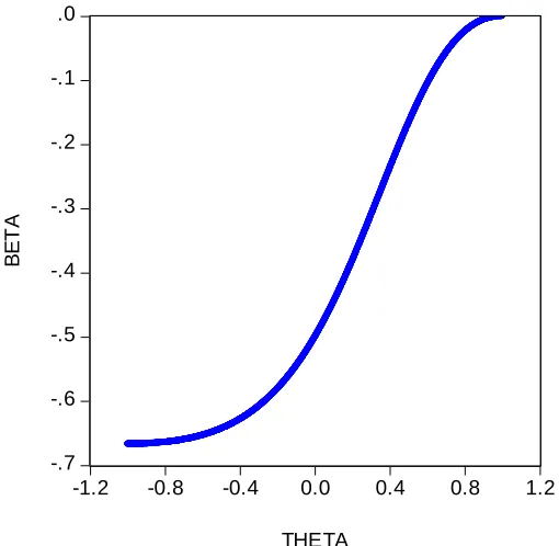
(a) When intuition follows an AR(1) process, with parameter , then ₁  and

2 2 

  . Substituting these two terms into equation (7) gives

2 1

  

 (8)

Clearly, when intuition is a stationary AR(1) process, that is, when ||1, then .

0 1 

 

(b) When intuition follows an MA(1) process, with parameter  , then 1 _{1 }2







0

2 

 . Substituting these terms into equation (7) gives

) 1 ( 2 ) 1 ( 2 2         

(iii) Ft|th Mt|th vt|th, with 0= 0 and 1 = 0.

In this case, where there is no correlation between current and past news and intuition, the expression for  is

1 0 2 2 2 2 1 0 2 2 2              

When a time series process is postulated for intuition, it is again most likely that the value of  is negative.

(iv) F_t|th M_t|th v_t|th, with ₀ 0 and ₁ = 0

In this case, where current intuition is correlated with current news, the parameter in (1) becomes 1 0 0 2 2 2 2 2 1 0 0 2 2 2 2 2                    

A typical macroeconomic variable would show positive autocorrelation, certainly for the first few of these so that, in practice, it is likely that ₂ 0. In this case for to become positive, ₀ should be large and negative.

In this most general case, for  > 0, it should hold that 2(10) is large and positive. With ₁ 0 and ₀ 0, the chances are high indeed that  0.

In summary, when there is no correlation between news and intuition, it is most likely that  0 . When there is a negative correlation between current news and current intuition, and when there is a positive correlation between past news and current intuition, it becomes more likely that  0. In the event that  0, this can be associated with the situation where the forecaster relies fully on an econometric model, and also where the forecaster relies fully on intuition, and where the time series properties of intuition are a random walk (that is,  1 in equation (8)). In contrast, when only intuition is used and intuition is a white noise process (that is,  0 in equation (8)), then  0.5.

4. Interpreting Table 1

With the results in the previous section, we can now evaluate the empirical results given in Table 1. It seems that theoretically the values of  can range from around -1 to , where the values in the range -0.5 to slightly positive seem to be most likely.

A value for  of -0.5 would mean that it is quite likely that the forecaster has discarded the outcome of the model, and has used intuition, with the peculiar property that there is zero correlation between v_t|th and v_{t|t(h1)}. This absence of correlation seems quite unusual, as the intuition-based forecasts are concerned with the same fixed event.

A large and positive value of  must mean that forecasters take current and one-period lagged news into account when forming their intuition. A negative correlation between current news and intuition (₀ 0) means that a forecaster downplays the relevance of current news, that is, there is under-reaction. This could be associated with a forecaster’s uncertainty with the most recent releases of data. A positive correlation between one-period lagged news and intuition (₁ 0) suggests that the forecaster amplifies a recent trend, which might not be there, and hence over-adjusts the model forecast. In the literature, these situations are all presented under the label of “forecast smoothing”.

The results in the previous section suggest that, based only on estimates of  , these separate cases cannot be disentangled. Various parameter configurations of

1 0 2 1

0, , , ,

 can lead to various values of .

By far, the optimal value of  is 0. This could mean either that the forecaster has relied fully on an econometric model, or that the forecast is given as

h t t h t

t v

F|_  |_

with

t h t t h t

t v

v|_  |_( _1) 

where _t ~(0,2) is a white noise process.

4. Conclusion

This paper has shown that the interpretation of  in a regression of forecast updates on past updates is not entirely straightforward. Currently, the literature unequivocally assigns meanings such as smoothing, and over-reaction or under-reaction, to certain values of , but we have shown in this paper that these are not one-to-one relationships.

In order to derive from the observed data on F_t|th what forecasters actually do, it is necessary to obtain estimates of the news process and of intuition. This requires fitting an econometric time series model for y_t to acquire estimates of _t. Next, this model can be used to create estimates of the model-based forecasts, M_t|th and, with these, one can estimate a time series with observations on intuition, v_t|th. These two estimated series can then be used to compute the correlations between intuition and current and past news. As such, one acquires estimates of the key parameters, ₀,₁,₂,₀,₁, and then one may sensibly interpret the value of the estimated  . As the variables are generated regressors, Franses, McAleer and Legerstee (2009) recommend using Newey-West HAC standard errors.

Table 1: Estimation Results for Variants of Equation (1)

Source Estimates of , with averaging or pooling

Clements (1997) -0.414 (average across 5 cases, GDP) Table 1, p. 233 -0.232 (average across 5 cases, inflation)

Isengildina et al. (2006) 0.396 (average across 5 cases, Corn) Table 2, p. 1097 0.212 (average across 5 cases, Soybeans)

Dovern and Weisser (2011) 0.089 (average across G7, GDP) Table 4, p. 463 -0.040 (average across G7, inflation)

0.001 (average across G7, industrial production) -0.021 (average across G7, private consumption)

Ager et al. (2009) 0.309 (average across 12 countries, GDP) Tables 5 and 6, 0.163 (average across 12 countries, inflation) pp. 178-179

-.7 -.6 -.5 -.4 -.3 -.2 -.1 .0

-1.2 -0.8 -0.4 0.0 0.4 0.8 1.2

THETA

B

E

T

A

References

Ager, P., M. Kappler, and S. Osterloh (2009), The accuracy and efficiency of the Consensus forecasts: A further application and extension of the pooled approach, International Journal of Forecasting, 25, 167-181.

Amir, E. and Y. Ganzach (1998), Overreaction and underreaction in analysts’ forecasts, Journal of Economic Behavior & Organization, 37, 333-347.

Ashiya, M. (2003), Testing the rationality of Japanese GDP forecasts: The sign of forecast revision matters, Journal of Economic Behavior & Organization, 50, 263-269.

Ashiya, M. (2006), Testing the rationality of forecast revisions made by the IMF and the OECD, Journal of Forecasting, 25, 25-36.

Batchelor, R. and P. Dua (1992), Conservatism and consensus-seeking among economic forecasters, Journal of Forecasting, 11, 169-181.

Berger, A.N. and S.D. Krane (1985), The informational efficiency of econometric model forecasts, Review of Economics and Statistics, 67, 667-674.

Capistran, C. and A. Timmermann (2009), Disagreement and biases in inflation expectations, Journal of Money, Credit and Banking, 41, 365-396.

Chang, C.-L., P.H. Franses and M. McAleer (2011), How accurate are government forecasts of economic fundamentals? The case of Taiwan, to appear in International Journal of Forecasting. Available at SSRN: http://ssrn.com/abstract=1431007.

Clements, M.P. (1997), Evaluating the rationality of fixed-event forecasts, Journal of Forecasting, 16, 225-239.

DellaVigna, S. (2009), Psychology and economics: Evidence from the field, Journal of Economic Literature, 47, 315-272.

Dovern, J. and J. Weisser (2011), Accuracy, unbiasedness and efficiency of professional macroeconomic forecasts: An empirical comparison for the G7, International Journal of Forecasting, 27, 452-465.

Franses, P.H. and R. Legerstee (2010), Do experts adjustments on model-based SKU-level forecasts improve forecast quality?, Journal of Forecasting, 29, 331-340.

Franses, P.H., M. McAleer and R. Legerstee (2009), Expert opinion versus expertise in forecasting, Statistica Neerlandica, 63, 334-346.

Gallo, G.M., C.W.J. Granger and Y. Jeon (2002), Copycats and common swings: the impact of the use of forecasts in information sets, IMF Staff Papers, 49, 4-21.

Isengildina, O., S.H. Irwin, and D.L. Good (2006), Are revisions to USDA crop production forecasts smoothed?, American Journal of Agricultural Economics, 88, 1091-1104.

Isiklar, G., K. Lahiri and P. Loungani (2006), How quickly do forecasters incorporate news? Evidence from cross-country surveys, Journal of Applied Econometrics, 21, 703-725.

Lawrence, M. and M. O’Connor (2000), Sales forecasting updates: How good are they in practice?, International Journal of Forecasting, 16, 369-382.

Loungani, P. (2001), How accurate are private sector forecasts? Cross-country evidence from consensus forecasts of output growth, International Journal of Forecasting, 17, 419-432.