Benchmarking of three dimensional multicomponent lattice Boltzmann equation

Benchmarking of three-dimensional multicomponent lattice Boltzmann equation

X. Xu,1,2,*K. Burgin,1M. A. Ellis,3and I. Halliday1

1_{Materials & Engineering Research Institute, Sheffield Hallam University, Howard Street, S1 1WB, UK}

2_{Department of Engineering and Mathematics, Sheffield Hallam University, Howard Street, S1 1WB, UK}

3_{Oriel College, University of Oxford, OX1 4EW, UK}

(Received 17 August 2017; revised manuscript received 25 October 2017; published 15 November 2017) We present a challenging validation of phase field multicomponent lattice Boltzmann equation (MCLBE) simulation against the Re=0 Stokes flow regime Taylor-Einstein theory of dilute suspension viscosity. By applying a number of recent advances in the understanding and the elimination of the interfacial microcurrent artefact, extending to a three-dimensional class of stability-enhancing multiple relaxation time collision models (which require no explicit collision matrix, note) and developing new interfacial interpolation schemes, we are able to obtain data that show that MCLBE may be applied in new flow regimes. Our data represent one of the most stringent tests yet attempted on LBE—one which received wisdom would preclude on grounds of overwhelming artefact flow.

DOI:10.1103/PhysRevE.96.053308

I. INTRODUCTION

The past two decades have seen steady growth in interest in multirelaxation time (MRT) lattice Boltzmann (LB) schemes, which offer enhanced simulation stability [1–8], etc. We extend to D3Q19 a recent D2Q9 variant [9], in which the usual collision matrix is only implicit, being represented by a carefully chosen, modal eigenbasis, which is subject to forced, scalar relaxation. As well as the usual advantages, the new method has transparent analytic properties: its orthogonal modes are defined as polynomials in the lattice basis, as are the elements of the transformation matrix between the distribution function and the mode space. This uniquely allows for the direct reconstruction of a post-collision distribution function, which is effectively parameterized by the eigenvalue spectrum. Our purpose in developing a new model is to stabilize multicomponent LBE (MCLBE) so as to attempt the challenge of recovering the Taylor-Einstein theory of suspension viscosity [10,11].

The structure of this paper is as follows. In Sec. II, we provide background material of the proposed 3D MRT scheme. In Sec.III, we present relevant methodological advances, in particular, the discovery of 19 polynomial expressions for the inverse transformation matrix, and the analysis of different viscosity interpolation methods. In Sec.IV, we illustrate and discuss the theoretical and simulation results achieved and finally, in Sec.V, we conclude on the significant findings of this work.

II. BACKGROUND

First, consider the base model. Our three-dimensional (3D) MRT LBE with body force,F, may be written

fi(x+ciδt,t+δt)

=fi(x,t)+

j Aij

f_j(0)(x,t)−fj(x,t)

+δt Fi, (1)

*_{Author to whom all correspondence should be addressed:}

xu.xu@shu.ac.uk

where

Fi =ti

3F·ci+9 2

1−λ3

2

(Fαuβ+Fβuα)

, (2)

and

f_j(0) =ρtj 1+3uαcj α+₂9uαuβcj αcjβ−3₂uγuγ

. (3) To recover hydrodynamics, Fi, collision matrix A, and its eigenvaluesλi, must preserve the following properties:

i

Fi=0,

i

ciFi =nF,

i

ciciFi = 1 2[C+C

T ],

i

1iAij =0,

i

ciαAij =0,

i

giAij =λ10gj,

i

ciαciβAij =λ4cj αcjβ,

i

giciαAij =λ11gjcj α,

i

c2_iαciβAij =λ14c2j αcjβ,

i

gic2iαAij =λ17gjc2j α, (4)

whereαandβ represent thex,y, orzdirections,λp denotes thepth eigenvalue ofAij, andCαβ≡1₂(uαFβ+uβFα) [9]. For eigenvalues, their corresponding left-row eigenvectors, h(p), p∈[0,18], and the modes they project, see TableI(a).Ais defined by its eigenspectrum (h(p)_,λ

p), which project modes with scalar relaxation.

III. METHODOLOGY A. Explicit algebraic 3D MRT scheme

For D3Q19, we extend the set developed for D2Q9 [9], using Gram-Schmidt orthogonalization to which in TableI(a). Four degenerate eigenvectors necessarily project hydrody-namic modes ρ≡_ifi andρu≡

ifici [9] withλi =0, six project components of stress Pαβ, four “ghosts” are chosen to projectN,J (following Refs. [2–4]) and five new eigenvectors are denoted E1,E2,E3,Xx, andXy. Left-row eigenvectorsh(p)_{sdefine projection matrix}

h(6) _h(6)

i =c

2

iz λ4 Pzz 1₂(Czz+Czz) (0)zz 6 −1 1 0

h(7) _h(7)

i =cixciy λ4 Pxy 1₂(Cxy+Cyx) (0)xy 7 0 1 0

h(8) _h(8)

i =cixciz λ4 Pxz 1₂(Cxz+Czx) (0)xz 8 1 1 0

h(9) _h(9)

i =ciyciz λ4 Pyz 1₂(Cyz+Czy) (0)yz 9 0 0 1

h(10) _h(10)

i =gi λ10 N 0 0 10 1 0 1

h(11) _h(11)

i =gicix λ11 Jx 0 0 11 0 1 1

h(12) _h(12)

i =giciy λ11 Jy 0 0 12 −1 0 1

h(13) _h(13)

i =giciz λ11 Jz 0 0 13 −1 0 1

h(14) _h(14)

i =c

2

ixciy λ14 E1 1₃Fy E1(0)=

1

3ρuy 14 0 0 −1

h(15) _h(15)

i =c2ixciz λ14 E2 13Fz E

(0)

2 =

1

3ρuz 15 1 0 −1

h(16) _h(16)

i =cixc2iy λ14 E3 1₃Fx E3(0)=

1

3ρux 16 0 1 −1

h(17) _h(17)

i =gic2ix λ17 Xx 1− λ₂4

(Fyuy+Fzuz) Xx(0)= ρ

2 u 2

y+u2z

17 −1 0 −1

h(18) _h(18)

i =gic2iy λ17 Xy 1− λ₂4

(Fxux+Fzuz) Xy(0)= ρ

2 u 2

x+u

2

z

18 0 −1 −1

such that

M f=(ρ,ρux,ρuy,ρuz,Pxx,Pyy,Pzz,Pxy,Pxz,Pyz, N,Jx,Jy,Jz,E1,E2,E3,Xx,Xy)T, (6) where f≡(f0,f1,f2, . . . ,f18)T. Using M, Eq. (1) may be

transformed to

M f+=M f+M A M−1(M f(0)−M f)+MF˜, (7) where ˜Fdenotes a column vector with elementsFi andf,f+ andf(0) _{are now column vectors. Since the h}(p) _{are left row}

eigenvectors ofA, it follows

M A= M ⇔ =M A M−1, (8) where =diag(λ₀, λ₁, . . . ,λ₁₈). Therefore, Eq. (1) may be written in mode space as

h(p)+=h(p)+λp(s(p)−h(p))+S(p), (9) whereS(p) ≡M·F˜ ands(p)≡M·f(0). The inverse transfor-mation matrix,

M−1≡(k(0),k(1),k(2), . . . ,k(18)), (10) may be constructed from column vectorsk(p), exactly defined as polynomials of the lattice basis, such that

6k_i(0)=ti

12giciθ2 −15ciθ2 −21c2iz+23−8gi

, (11)

k(1)_i =ti[6cixciy(2cix−ciy)+cix(5+gi)−2ciy(2−gi)], (12)

k_i(2,3)=ticiγ

5+gi−6c2ix

, (13)

2k(4_i ,5)=ti

−2gi c2iζ+2ciξ2

+11c2_iζ+c2_iξ +3c2_iz−5+2gi

,

(14)

2k_i(6)=ti

−6gic2iθ+3c

2

iθ+15c

2

iz−7+4gi

,

k_i(7,...,9)=3ticiαciβ, (15)

2k_i(10)=ti

6c_iθ2 −12gic2iθ+12c2iz−8+11gi

, (16)

k(11)_i =ti[3cixciy(2cix−ciy)+cix(1+2gi)−ciy(2+gi)], (17)

k_i(12,13)=2tigiciγ

2+4gi−6cix2

, (18)

k_i(14,15)=3ticiγ

6c2_ix−2−gi

, (19)

k_i(16)=3ti[6cixciy(ciy −2cix)− (2+gi)(cix−2ciy)], (20)

k_i(17)=ti

−gi 4c2ix+c

2

iy

−c2_ix−2c2_iy−3c2_iz+2−2gi

,

FIG. 1. Viscous stress fieldσxy in the equatorial plane of a spherical red drop, radiusR=20, suspended in a blue fluid which is sheared,

at Re=0 for two viscosity ratios, , withηB = 1₃ (continuous component) and R_L = 1₆. Case 1, = ₁₆1: (a) Taylor’s theory, (b) interfacial

interpolation based upon a density-weighted harmonic mean of separated fluids’ parameterτ= 1

λ4 [see Eq. (27)], (c) interfacial interpolation

based upon a density-weighted harmonic mean of shear viscosity [see Eq. (28)], and (d) interfacial interpolation based upon a density-weighted arithmetic mean of shear viscosity [see Eq. (29)]. Case 2, =12: (e) Taylor’s theory, (f) interfacial interpolation based upon a density-weighted harmonic mean of separated fluids’ parameterτ= _λ41 [see Eq. (27)], (g) interfacial interpolation based upon a density-weighted harmonic mean of shear viscosity [see Eq. (28)], and (h) interfacial interpolation based upon a density-weighted arithmetic mean of shear viscosity [see Eq. (29)].

k_i(18)=ti

2gi c2ix+2c2iy

−2c2_ix−c_iy2 −3c2_iz+2−2gi

,

(22) wherec2

iθ =cix2 +c2iy,γ ∈[y,z] and is taken in alphabetical order, (ζ,ξ) are taken in order as (x,y) and (y,x), and α,β∈[x,y,z] are denoted in the pair order of (x,y), (x,z), and (y,z). Using the methodology developed for the D2Q9 case [9], we invertMto construct a post-collision distribution function vectorf+, describing flow in the presence of force distribution,F:

f+=M−1(ρ+,ρu+_x,ρu+_y,ρu_z+,P_xx+,P_yy+,P_zz+,P_xy+,P_xz+, P_yz+,N+,J_x+,J_y+,J_z+,E₁+,E₂+,E₃+,X_x+,X+_y)T, (23) which may be written in explicit form after Ref. [9]. MRT LBE is more computationally expensive than LBGK [12] but is more stable [1–3]. The scheme we extend here from Ref. [9] includes the existence of polynomial expressions k(p)_{, which allow (i) algebraic inversion from the mode space}

[Eq. (10)], (ii) an exact expression for f+, (iii) removal of explicit collision and inversion matrices, and hence some computational overhead.

B. Interfacial viscosity interpolation

Here we are motivated by a need to extend the viscosity con-trast available in simulations of multicomponent flow using a phase-field MCLBE [9,13,14], to facilitate a validation against

the stress field Taylor predicted in 1932, for steady, shear flow past a spherical drop at Re=0 [10] and the consequent prediction of effective viscosity in a dilute suspension of small drops, after Einstein [11]. Accordingly,

F= σ κ 2 ∇ρ

N

(24)

is an immersed boundary force, where according to Ref. [15], the phase field is

ρN≡ ρR−ρB ρR+ρB

, (25)

and the local interfacial curvature is

κ≡∇s

∇ρN

|∇ρN_|. (26)

Here, ρR and ρB are densities of two immiscible fluid components, which are segregated, post collision, using the methodology of d’Ortona [16] (see Refs. [9,13,14]) and∇sis a surface gradient operator.

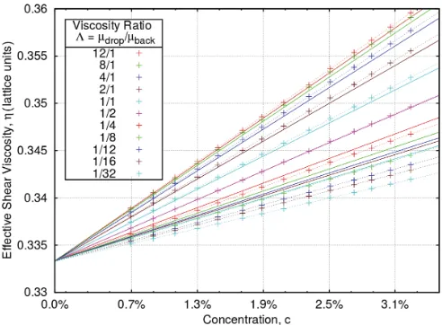
FIG. 2. Effective suspension viscosity, ηeff, as a function of

concentration, c (discrete crosses linearly interpolated by dotted lines), for the indicated range of drop/background fluid viscosity ratio,

= ηR

ηB, together with the variation predicted by the Taylor-Einstein

result,η_eff(T)=ηB[1+( 5 2ηR+ηB

ηR+ηB )c] (continuous line of corresponding

color). These data were obtained using the interpolation defined in Eq. (27).

dynamic conditions. In the present context, we are concerned with the no-traction condition [17].

Take a steady, planar, red-blue interfacex=x₀, constant, sheared inydirection, after Liuet al.[18]. Phase field MCLBE is described by a weakly compressible Navier-Stokes equation with F, for what is a single, effective fluid (the role of F is to insert Laplace law physics). For a flat interface,F=0 and the lattice fluid is described by _dxd σ_xy =0,∀x. Applying system symmetries, we obtainσ_xy =K, a constant∀x. This prefigures the continuum no-traction (continuity of viscous flux) condition. Apparently, LBE’s dynamics automatically ensure shear stress is continuous through the interface region. Clearly, choice exists in the interpolation of viscosity or, equivalently, λ4. Liu and coworkers impose a requirement

on the velocity gradient, which it varies like ρN [18], in this situation and in applications to contact angle hysteresis [19]. This assumption yields an interpolation of λ4 derived

from the harmonic mean of viscosity with weights ρR

ρ and ρB

ρ. Liu et al. [18] state their approach is equivalent to Ginzburg’s, when projecting the sharp interface limit [20] (see Fig. 3 of Ref. [20]). Zuet al.[21] assume the interfacial velocity gradient follows an order parameter and argue for an interpolation based on a weighted arithmetic average of reciprocal viscosity. There are more involved approaches, including that of Grunauet al.[22]. For the data presented in the next section, optimum agreement with Taylor-Einstein theory is obtained using an alternative method.

In our MCLBE, interfacial effects are carried by a force with weight|∇ρN_{|, which may be approximated by} 4ρRρB

ρ2 =

(1−ρN2_{) [23]. Self-consistency argues for an interpolation of}

λ₄, between bulk valuesλR

4 andλ

B

4, such that source term,Fi, has a consistent variation. Hence, we choose (1−λ4

2)∼ρ

N_or (1−λ¯4

2)=

ρR

ρ(1− λR

4

2)+

ρB

ρ(1− λB

4

2), and noting

ρR

ρ + ρB

ρ =

and also an interpolation based on the arithmetic mean of shear viscosityη= ρR

ρηR+ ρB

ρηB, which may be expressed as

1 ¯ λ₄ =

ρR ρ

1 λR

4

+ρB ρ

1 λB

4

. (29)

IV. RESULTS AND DISCUSSION

Experimental studies of suspension viscosity emphasize concentration values outside the Re=0 theory but do identify certain emulsions that behave in agreement with the Taylor-Einstein result, certainly for concentrationsc <5% (see, e.g., Nawab et al. [24], Hur et al. [25], and Masonet al. [26]). Notably, a comparison of MCLBE with Re=0 theory is not obstructed by MCLBE’s notorious interfacial microcurrent (see Ref. [27] and references therein). For phase-field MCLBE variants, this artefact has recently been argued to arise from superposable solutions to the field equations, attributable, in increasing significance, to the stencil used for force weight

∇ρN_{, discrete lattice effects, and (most significantly) the} calculation ofκ[27]. At Re=0, hydrodynamic signals cannot be assumed to overwhelm artefacts, but this regime may still be addressed by subtracting independent microcurrent fields, to expose a hydrodynamic response. (Micro-current fields are easily determined for a red drop in stationary blue fluid.)

Figure1compares stresses between theory and microcur-rent adjusted simulation. We show viscous stressσ_xy measured in the projected equatorial plane,z=0, of a three-dimensional red drop, initial radiusR=20 lattice units, contained within a cubic box, sideLlattice units, with the continuous component (blue) fluid subject to a Lees-Edwards shear [28]. This boundary condition eliminates finite-size effects but allows periodic drop replicas to interact [9]. The resulting suspension concentration is controlled byL, i.e.,

c= 4π R

3

3L3 . (30)

The applied shear corresponds to approximately constant boundary flow parallel to ˆey in box faces x =x0, constant.

Taylor calculated σ_αβ(T), α,β∈[x,y,z] due to an inclined, applied shear, superposed with a constant body rotation around ˆez [10]. Accordingly, to compare with our simu-lation, it is necessary to rotate coordinates and Fig. 1(a)

shows a combination of Taylor’s stresses (σ(T)

FIG. 3. Data equivalent to that shown in Fig.2using different interfacial interpolation methods. Effective suspension viscosity,ηeff,

as a function of concentration,c(discrete crosses linearly interpolated by dotted lines), for the indicated range of drop/background fluid viscosity ratio, = ηR

ηB, together with the variation predicted by the

Taylor-Einstein result,η(_effT)=ηB[1+( 5 2ηR+ηB

ηR+ηB )c] (continuous line of

corresponding color). These data were obtained using an interpolation based upon (a) the harmonic mean of the separated fluids’ shear viscosity defined in Eq. (28) and (b) the arithmetic mean of shear viscosity defined in Eq. (29).

L=128, viscosity contrast:

≡ ηR ηB

, (31)

whereηCis the shear viscosity of theCfluid. In Fig.1we show the significant difference between stress fields measured using existing and alternative interfacial interpolations of viscosity, or equivalently,λ4. These are given in Eqs. (27), (28), and (29).

Furthermore, the viscous stress field,σ_xy , is shown in Fig.1

for two . For this data,ηB= 1₃ (the continuous component) is fixed andR_L = 1₆. For the images in the upper row, =₁₆1. Figure 1(a) shows Taylor-Einstein theory; Fig. 1(b) shows

FIG. 4. Relative error of interfacial interpolation method,, for a range of , expressed in percentage. For all data in Fig. 2, ≡ η

(T) eff−ηeff

η_eff(T) ×100% was computed for each of the three interfacial

interpolation methods considered, as identified in the key.

the stress field obtained using the interfacial interpolation based upon a density-weighted harmonic mean of separated fluids’ parameter τ =_λ1

4 [see Eq. (27)]; Fig. 1(c) shows

stress obtained with the interfacial interpolation based upon a density-weighted harmonic mean of shear viscosity [see Eq. (28); and Fig. 1(d) shows results from our method of interfacial interpolation shear viscosity, based upon a density-weighted arithmetic mean of shear viscosity [see Eq. (29)]. In the top row, it is clear that Figs. 1(b) and1(d) are most representative of Fig.1(a). The bottom row in Fig.1 shows equivalent data for =12 and it clearly shows that Figs.1(f)

and1(g)are most representative of Fig.1(e).

We next consider a range of crystalline suspension concen-trations, each of fixed viscosity ratio, , inferring effective suspension viscosity,η_eff, from plots of system-averagedσxy against c, fitted using unconstrained regression (see, e.g., Fig.2). For microcurrent flow alone,σxy ≈0 (though viscous dissipation is affected—see Ref. [9]) but it is still necessary to correct systemσxy for the presence of immersed boundary force,F[9]. Agreement with Taylor-Einstein theory is affected by the method used to interpolateλ4, or alternatively viscosity,

η, in the interfacial region, as we now discuss. All data in Figs.2,3, and4correspond to

Re≡ γ R˙

2_ρ

η =0.0198, (32)

Ca≡ηγ R˙

σ =0.0110, (33) which are held constant throughout.

Figure2shows 11 sets of measuredηeff for a wide range

of such that ₃₂1 12 (crosses interpolated by dotted lines), and the appropriate Taylor-Einstein predictions (solid lines of same color):

η(_effT) =ηB

1+ ₅

2 +1

+1

c

. (34)

Eq. (27) represents an optimum over the whole range of . This point is further summarized in Sec.V.

V. CONCLUSIONS

Taken together, Figs.1–4 underscore the significance of the interfacial interpolation. The fit produced by Eq. (27) represents an optimum over the range of studied and is best when the exterior fluid is more viscous. For <1, the fit is improved by using an interpolation based upon an arithmetic mean of viscosities however the fit at >1 then degrades. Over the range of , the scheme in Eq. (27) produced most consistent agreement.

Comparison with the Taylor-Einstein represents a stringent test of phase field MCLBE (and thereby the approximations

a solution of the Stokes equation) therefore superpose with flow induced by the applied shear. Once identified, they may be subtracted. Furthermore, this work points to the importance of the method of interpolation of viscosity eigenvalue, λ₄, across the interfacial region, with our data producing a optimum for the interpolation in Eq. (27).

ACKNOWLEDGMENTS

M.A.E. gratefully acknowledges financial support from the Engineering and Physical Sciences Research Council, Swindon, UK via a summer bursary from Collaborative Computational Project 5, Grant Reference EP/M022617/1 and Oriel College, University of Oxford.

[1] P. Lallemand and L.-S. Luo,Phys. Rev. E61,6546(2000). [2] R. Benzi, S. Succi, and M. Vergassola,Europhys. Lett.13,727

(1990).

[3] R. Benzi, S. Succi, and M. Vergassola, Phys. Rep.222, 145 (1992).

[4] P. J. Dellar,Phys. Rev. E65,036309(2002).

[5] M. E. McCracken and J. Abraham,Phys. Rev. E71,036701 (2005).

[6] K. N. Premnath and J. Abraham, J. Comput. Phys.224,539 (2007).

[7] R. Du, B. Shi, and X. Chen,Phys. Lett. A359,564(2006). [8] A. Fakhari and T. Lee,Phys. Rev. E87,023304(2013). [9] I. Halliday, X. Xu, and K. Burgin, Phys. Rev. E95, 023301

(2017).

[10] G. I. Taylor,Proc. Roy. Soc.138,41(1932). [11] E. Einstein,Ann. Physik.19,371(1906).

[12] Y. H. Qian, D. d’Humières, and P. Lallemand,Europhys. Lett. 17,479(1992).

[13] H. Liu, A. J. Valocchi, and Q. Kang,Phys. Rev. E85,046309 (2012).

[14] Y. Ba, H. Liu, J. Sun, and R. Zheng,Phys. Rev. E88,043306 (2013).

[15] S. V. Lishchuk, C. M. Care, and I. Halliday,Phys. Rev. E67, 036701(2003).

[16] U. D’Ortona, D. Salin, M. Cieplak, R. B. Rybka, and J. R. Banavar,Phys. Rev. E51,3718(1995).

[17] L. Landau and E. M. Lifshitz, Fluid Mechanics, 2nd ed. (Pergamon Press, Oxford, UK, 1966)

[18] H. Liu, A. J. Valocchi, C. Werth, Q. Kang, and M. Oostrom, Adv. Water Resour.73,144(2014).

[19] H. Liu, Y. Ju, N. Wang, G. Xi, and Y. Zhang,Phys. Rev. E92, 033306(2015).

[20] I. Ginzburg,J. Stat. Phys.126,157(2007).

[21] Y. Q. Zu and S. He,Phys. Rev. E87,043301(2013).

[22] D. Grunau, S. Chen, and K. Eggert, Phys. Fluids A5, 2557 (1993).

[23] T. J. Spencer, I. Halliday, and C. M. Care,Phys. Rev. E82, 066701(2010).

[24] M. A. Nawab and S. G. Mason,Trans. Faraday Soc.54,1712 (1958).

[25] B. K. Hur, C. B. Kim, and C. G. Lee, J. Ind. Eng. Chem.6, 318 (2000).

[26] T. G. Mason, J. Bibette, and D. A. Weitz,J. Colloid Interface Sci.179,439(1996).

[27] I. Halliday, S. V. Lishchuk, T. J. Spencer, K. Burgin, and T. Schenkel,Comput. Phys. Commun.219,286(2017).