Origin of terminal voltage variations due to self mixing in terahertz frequency quantum cascade lasers

GRIER, Andrew, DEAN, Paul, VALAVANIS, Alexander, KEELEY, James,

KUNDU, Iman, COOPER, Jonathan D, AGNEW, Gary, TAIMRE, Thomas, LIM,

Yah Leng, BERTLING, Karl, RAKIC, Aleksander D, LI, Lianhe H, HARRISON,

Paul <http://orcid.org/0000-0001-6117-0896>, LINFIELD, Edmund H, IKONIC,

Zoran, DAVIES, A. Giles and INDJIN, Dragan

Available from Sheffield Hallam University Research Archive (SHURA) at:

http://shura.shu.ac.uk/13265/

This document is the author deposited version. You are advised to consult the

publisher's version if you wish to cite from it.

Published version

GRIER, Andrew, DEAN, Paul, VALAVANIS, Alexander, KEELEY, James, KUNDU,

Iman, COOPER, Jonathan D, AGNEW, Gary, TAIMRE, Thomas, LIM, Yah Leng,

BERTLING, Karl, RAKIC, Aleksander D, LI, Lianhe H, HARRISON, Paul, LINFIELD,

Edmund H, IKONIC, Zoran, DAVIES, A. Giles and INDJIN, Dragan (2016). Origin of

terminal voltage variations due to self-mixing in terahertz frequency quantum

cascade lasers. Optics Express, 24 (19), 21948-21956.

Copyright and re-use policy

See

http://shura.shu.ac.uk/information.html

Sheffield Hallam University Research Archive

Origin of terminal voltage variations due to

self-mixing in terahertz frequency quantum

cascade lasers

A

G

,

P

D

,

A

V

,

J

K

,

I

K

,

J

D. C

,

G

A

,

T

T

,

Y

L

L

,

K

B

,

A

D. R

,

L

H. L

,

P

H

,

E

H. L

,

Z

I

,

A. G

D

,

D

I

1_{School of Electronic and Electrical Engineering, University of Leeds, Leeds LS2 9JT, UK}

2_{School of Information Technology and Electrical Engineering, University of Queensland, Brisbane 4072,} Australia

3_{School of Mathematics and Physics, The University of Queensland, Brisbane QLD 4072, Australia} 4_{Materials and Engineering Research Institute, Sheffield Hallam University, Sheffield S1 1WB, UK} 5_{atgrier4@gmail.com}

6_{p.dean@leeds.ac.uk} 7_{d.indjin@leeds.ac.uk}

Abstract: We explain the origin of voltage variations due to self-mixing in a terahertz (THz)

frequency quantum cascade laser (QCL) using an extended density matrix (DM) approach. Our DM model allows calculation of both the current–voltage (I–V) and optical power characteristics of the QCL under optical feedback by changing the cavity loss, to which the gain of the active region is clamped. The variation of intra-cavity field strength necessary to achieve gain clamping, and the corresponding change in bias required to maintain a constant current density through the heterostructure is then calculated. Strong enhancement of the self-mixing voltage signal due to non-linearity of the (I–V) characteristics is predicted and confirmed experimentally in an exemplar 2.6 THz bound-to-continuum QCL.

Published by The Optical Society under the terms of theCreative Commons Attribution 4.0 License. Further distribution of this work must maintain attribution to the author(s) and the published article’s title, journal citation, and DOI.

OCIS codes:(170.6795) Terahertz imaging; (120.3180) Interferometry; (140.5965) Semiconductor lasers, quantum

cascade.

Referencesand Links

1. L. Li, L. Chen, J. Zhu, J. Freeman, P. Dean, A. Valavanis, A. G. Davies, and E. H. Linfield, “Terahertz quantum cascade lasers with >1 W output powers,” Electron. Lett50(2), 309–311 (2014).

2. S. Fathololoumi, E. Dupont, C. Chan, Z. Wasilewski, S. Laframboise, D. Ban, A. Mátyás, C. Jirauschek, Q. Hu, and H. C. Liu, “Terahertz quantum cascade lasers operating up to∼200 K with optimized oscillator strength and

improved injection tunneling,” Opt. Express20(4), 3866–3876 (2012).

3. M. Tonouchi, “Cutting-edge terahertz technology,” Nat. photonics1, 97–105 (2007).

4. Y. Lee,Principles of terahertz science and technology(Springer Science & Business Media, 2009).

5. P. Dean, A. Valavanis, J. Keeley, K. Bertling, Y. L. Lim, R. Alhathlool, A. D. Burnett, L. H. Li, S. P. Khanna, D. Indjin, T. Taimre, A. D. Rakić, E. H. Linfield, and A. G. Davies, “Terahertz imaging using quantum cascade lasers–a review of systems and applications,” J. Phys. D: Appl. Phys.47(37), 374008 (2014).

6. D. Kane and K. A. Shore,Unlocking Dynamical Diversity: Optical Feedback Effects on Semiconductor Lasers(John

Wiley & Sons, 2005).

7. E. Lacot, O. Jacquin, G. Roussely, O. Hugon, and H. G. De Chatellus, “Comparative study of autodyne and heterodyne laser interferometry for imaging,” J. Opt. Soc. Am. A27(11), 2450–2458 (2010).

8. R. Lang and K. Kobayashi, “External optical feedback effects on semiconductor injection laser properties,” IEEE J. Quant. Electron.16(3), 347–355 (1980).

#269929 http://dx.doi.org/10.1364/OE.24.021948

9. J. A. Roumy, J. Perchoux, Y. L. Lim, T. Taimre, A. D. Rakić, and T. Bosch, “Effect of injection current and temperature on signal strength in a laser diode optical feedback interferometer,” Appl. Opt.54(2), 312–318 (2015).

10. T. Taimre, M. Nikolić, K. Bertling, Y. L. Lim, T. Bosch, and A. D. Rakić, “Laser feedback interferometry: a tutorial on the self-mixing effect for coherent sensing,” Adv. Opt. Photon.7(3), 570–631 (2015).

11. K. Bertling, Y. L. Lim, T. Taimre, D. Indjin, P. Dean, R. Weih, S. Hofling, M. Kamp, M. von Edlinger, J. Koeth, and A. D. Rakić, “Demonstration of the self-mixing effect in interband cascade lasers,” Appl. Phys. Lett.103, 231107

(2013).

12. R. Juškaitis, N. Rea, and T. Wilson, “Semiconductor laser confocal microscopy,” Appl. Opt33, 578–584 (1994).

13. A. Valavanis, P. Dean, Y. L. Lim, R. Alhathlool, M. Nikolic, R. Kliese, S. Khanna, D. Indjin, S. Wilson, A. Rakić, E. Linfield, and G. Davies, “Self-mixing interferometry with terahertz quantum cascade lasers,” IEEE Sensors J.

13(1), 37–43 (2013).

14. P. Dean, A. Valavanis, J. Keeley, K. Bertling, Y. Leng Lim, R. Alhathlool, S. Chowdhury, T. Taimre, L. H. Li, D. Indjin, S. J. Wilson, A. D. Rakić, E. H. Linfield, and A. Giles Davies, “Coherent three-dimensional terahertz imaging through self-mixing in a quantum cascade laser,” Appl. Phys. Lett.103, 181112 (2013).

15. P. Dean, Y. L. Lim, A. Valavanis, R. Kliese, M. Nikolić, S. P. Khanna, M. Lachab, D. Indjin, Z. Ikonić, P. Harrison, A. D. Rakić, E. H. Linfield, and A. G. Davies, “Terahertz imaging through self-mixing in a quantum cascade laser,” Opt. Lett.36(13), 2587–2589 (2011).

16. T. V. Dinh, A. Valavanis, L. J. M. Lever, Z. Ikonić, and R. W. Kelsall, “Extended density-matrix model applied to silicon-based terahertz quantum cascade lasers,” Phys. Rev. B85(23), 235427 (2012).

17. H. Callebaut and Q. Hu, “Importance of coherence for electron transport in terahertz quantum cascade lasers,” J. Appl. Phys.98, 104505 (2005).

18. M. Franckié, D. O. Winge, J. Wolf, V. Liverini, E. Dupont, V. Trinité, J. Faist, and A. Wacker, “Impact of interface roughness distributions on the operation of quantum cascade lasers,” Opt. Express23(4), 5201–5212 (2015).

19. A. Grier, “Data associated with Origin of terminal voltage variations due to self-mixing in terahertz frequency quantum cascade lasers,” University of Leeds data repository (2016) http://doi.org/10.5518/77.

20. A. D. Rakić, T. Taimre, K. Bertling, Y. L. Lim, P. Dean, D. Indjin, Z. Ikonić, P. Harrison, A. Valavanis, S. P. Khanna, M. Lachab, S. J. Wilson, E. H. Linfield, and A. G. Davies, “Swept-frequency feedback interferometry using terahertz frequency QCLs: a method for imaging and materials analysis,” Opt. Express21(19), 22194–22205 (2013).

1. Introduction

Quantum cascade lasers (QCLs) are compact semiconductor sources of terahertz (THz) frequency radiation that are capable of emission powers of up to 1 W [1] and maximum operating temperatures of 200 K [2]. Owing to the transparency of many materials to THz radiation, coupled with its unique interaction with inter- and intra-molecular bonds in both organic and inorganic materials, a number of potential applications of these sources have been proposed including security screening, medical imaging, atmospheric science, and pharmaceutical monitoring [3, 4]. In particular, the use of laser feedback interferometry (LFI) with QCL sources has received significant attention since it enables a wide range of coherent sensing applications without requiring a separate detector, and therefore simplifies experimental systems significantly [5].

LFI (based on the self-mixing (SM) effect) refers to the partial reinjection of the radiation emitted from a laser after reflection from a target; the injected radiation field interacts with the intra-cavity field causing a change in the operating parameters of the laser. These changes are required in order to maintain the field continuity across the laser facet-external cavity boundary, and in the case of semiconductor lasers, result in a measurable variation of the laser terminal voltage. This phenomenon has underpinned a wide range of sensing and imaging applications [6,7]. As such, an accurate physical understanding of the relationship between this SM voltage signal and the optical feedback from an external cavity is of great importance.

laser structure, and can vary from the microvolt level for diode lasers to the millivolt level for THz QCLs.

To address this problem we have developed a comprehensive model that accounts for the laser structure in order to obtain quantitative information about the expected magnitude of the self-mixing voltage signal in THz QCLs. Whilst the Lang–Kobayashi model enables the dynamic state populations and light interaction to be modelled, a linear relationship between the change in intracavity light power,∆P, and terminal voltage variationV_SMis commonly assumed [12–14], i.e.

V_SM∝∆P. (1)

However, this assumption is not strictly applicable to QCL structures since carrier transport is dominated by the mechanisms of electron subband alignment, intersubband scattering, and photon driven transport between subbands with energy separations that change with applied bias (terminal voltage). Indeed, previous experimental observations based on a bound-to-continuum (BTC) QCL structure (see Fig. 2(b) in Ref. [15]) have shown SM voltage signal to be greatest near threshold and to decrease with greater driving currents, which suggests a non–linear relationship betweenV_SM and optical power, P. Further evidence of the limitation of this conventional approach is shown in the present work, in which we demonstrate a QCL device that departs significantly from the assumed linear behavior. We observe, both theoretically and experimentally, strong enhancement of the self-mixing signal in regions where the local gradient of theI–V curve (differential resistance) increases.

Here we use an extended density matrix (DM) formalism to calculate the current–voltage characteristics of a BTC QCL emitting at 2.6 THz and predict the effect of feedback variation on the terminal voltage at a fixed drive current. The density matrix approach is capable of including coherent transport due to tunnelling as well as the effect of the cavity light field on current during lasing. This approach is shown to predict well the magnitude of the experimental self-mixing signal. The full details of the DM model are described in Ref. [16] although here we reiterate some relevant details for clarity of the present work.

2. Density matrix model

In our model, three consecutive periods of the QCL are considered. First, basis eigenstates are determined using a tight-binding Hamiltonian, in which each period of the QCL potential profile is “padded” within thick barriers such that the electrons are confined within a single period.

An extended Hamiltonian matrix is then generated to describe the interactions between each pair of states. The diagonal terms contain the state energies calculated using the tight-binding Hamiltonian, and the inter-period terms contain the Rabi oscillation strengths calculated as

~Ωi j ≈ hi|Hext−HTB|ji [17] wherei,j are state indices and the terms Hext and HTB refer

to the Hamiltonians (potentials) of the extended structure and of the “tight-binding” sections, respectively. Interaction with the light field present in the cavity is included in the Hamiltonian with off-diagonal intra-period terms given by [16]:

Hi,j =zi,jA0eiω0t, (2)

whereω₀is the frequency of the optical cavity field,tis time,zi,j is the dipole matrix element

for the transition, andA₀is the intensity of the cavity optical field.

assumed to have three harmonic terms such that

ρi,j =ρ+i,jexp(iω0t)+ρDCi,j +ρ −

i,jexp(−iω0t). (3)

A relaxation matrix is included in the Liouville equation, which describes the damping of the system. This contains both intra- and inter- subband lifetimes with scattering rate contributions from alloy disorder, acoustic phonons, longitudinal optical (LO) phonons and ionized impurities. Interface roughness scattering is also included with an r.m.s. roughness height∆=2.5 Å and

correlation lengthΛ=100 Å, similar to that estimated elsewhere [18].

The current density is extracted from the solved density matrix as j =Tr(ρJ)/2, with the

current matrix derived from the average drift velocity as

J=ei

~[

H,z] , (4)

whereHis the Hamiltonian matrix,zis a matrix containing dipole transition elements, andeis the electron charge. Gain is extracted fromJby calculating the complex permittivity as described

in Ref. [16].

For each value of applied bias (field) a fully self-consistent simulation is performed and the light field strength (A₀) iterated until gain is clamped to a defined loss. Variation of the cavity loss (and therefore the clamped optical field strength) affects current via the off-diagonal intra-period Hamiltonian terms in Eq. (2) which also affect the time-dependent coherences in Eq. (3). The intra-cavity optical power is calculated as

P= cnwh0

2 |A0|2, (5) where₀,n,w, andhare the vacuum permittivity, refractive index, width, and thickness of the active region respectively.

3. Free-running QCL characteristics

A BTC QCL emitting at 2.6 THz was driven using a dc current source. The device used here has the same active region design and semi-insulating surface plasmon waveguide as the structure described in Ref. [15], although was processed from a different wafer and with ridge dimensions 2.4 mm×150 µm×11 µm. The device was cooled using a continuous-flow helium cryostat and

maintained at a constant heat-sink temperature of 35 K. Radiation from the laser was collimated using an off-axis paraboloidal (OAP) reflector and modulated at a frequency of 210 Hz using a mechanical chopper. The free-running relationship between THz power and bias voltage (P–V) was measured by focusing the THz beam into a helium-cooled Ge:Ga photoconductive detector using a second OAP and recording the time-averaged signal via a lock-in amplifier synchronized to the modulation frequency. A THz photoacoustic power meter was used to calibrate measured values. The free-running current–voltage (I–V) characteristics were recorded simultaneously.

Good agreement was achieved between the experimentalP–I–V characteristics and our DM simulation by including a free-running loss of LFR = 16.1 cm−1, an Ohmic contact resistance

of 1.57Ωand photodetector collection efficiency of 48 %, as shown in Fig. 1 and included in

Dataset 1[19]. These simulations were carried out with a lattice temperature of 50 K to account

Current density (A/cm

2

)

190

200

210

220

230

240

250

260

270

Bias

(V)

2.6

2.8

3

3.2

3.4

3.6

3.8

4

Density matrix

Experimental

Power (mW)

0

1

2

3

4

5

6

7

Figure 1. Comparison of calculated and experimentalP–IandV–Icurves for a heat sink temperature of 35 K. A contact resistance of 1.57Ωis applied to the density matrixI–Vdata simulated for a lattice temperature of 50 K.

To account for this in the model (in which the structure is biased with an applied field) the output power is set to zero, and current is asserted to increase a negligible amount (fitted with experiment), in NDR regions. Other experimental effects include contact resistance, contact voltage drops, parasitic currents and device heating. Therefore it can be necessary to link the current–light response calculated by the DM model with the measuredI–V curve. Current/loss dependencies of this “hybrid” approach are discussed further in Section 5.

4. Self-mixing interferometry

An experimental LFI system was configured by reflecting the collimated THz beam back along the same optical path into the QCL cavity using a planar mirror, forming a nominal external cavity length of 40 cm. The resulting interference between the intra-cavity and reflected THz fields causes a small change in the emission frequency of the QCL such that the field is continuous across the facet-external cavity boundary. The feedback also gives rise to changes in the photon and electron density within the laser cavity, and this was observed as a perturbation to the terminal voltageV_SM, which was monitored via a lock-in amplifier synchronized to the chopper modulation frequency. In order to recover the maximum magnitude of voltage perturbation for each operating current, the phase of the reflected field was adjusted by varying the path length of the external cavity within one interference fringe.

3

2.5

Bias (V)

2

1.5

1

10

15

Loss (1/cm)

20

100

0

300

200

25

Current density (A/cm

2

)

2.6

2.4

Bias (V)

2.2

2

1.8

1.6

10

15

Loss (1/cm)

20

0

5

15

10

25

Optical power (mW)

b)

a)

insight into the effects of the feedback level on the electron transport in the device and the resulting variations in the laser voltage and current. Experimentally, the QCL was driven at a fixed current and the terminal voltage was measured. However, in our electron transport model the applied field and cavity loss are inputs to the model, while current is a calculated output. To account for this an inverse interpolation of the bias–loss–current-density characteristic was performed to determine the equivalent field applied across the device for each current and cavity loss value. For example, if the QCL is lasing and cavity loss is decreased, then the optical field will increase to balance gain and loss. This increases stimulated emission current; however since the total current is fixed, the active region bias simultaneously decreases to compensate with decreased injection alignment. To obtain the computed data necessary for interpolation inversion, optical output power and current density were calculated between fields of 0–2.5 kV/cm and cavity losses of 10–25 cm−1_{(i.e. a range around the free-running loss determined in Section 3)}

and the results are plotted in Fig. 2. The self-mixing signal,VSM, can then be obtained from

interpolation of these data, at each current, as:

VSM(I)=|V(I,LFR)−V(I,LFR+∆L)|, (6)

whereL_FR and∆Lare the free-running loss and change in loss due to SM respectively. The appropriate value of∆Lis dependent on the experimental setup and is affected by many factors such as the reinjection coupling efficiency, changing emission frequency, mode formation, and dynamic effects. Direct calculation of∆Lis beyond the scope of the present work, where the origin of terminal voltage is of interest. The value of ∆L is therefore chosen by fitting the magnitude ofV_SMwith experimental observations.

5. Results

Figure 3 shows experimental and theoreticalV_SM(I)characteristics of the SM response. A fitted

value of∆L=−1.4 cm−1is shown to provide excellent agreement for the signal amplitude over

a large range of operating currents. Nevertheless, we note that∆L=−0.3 cm−1corresponds to

a power modulation of approximately 5 %, which is consistent with that observed experimen-tally [13]. In both the simulated and experimental data, a strong enhancement of the SM signal occurs near where the QCL turns off due to the onset of the NDR region atI≈257 A/cm2.

We propose that the largeV_SMsignal observed here is due to the large QCL field perturbation required to achieve a subband alignment such that the total of the scattering/tunneling current and stimulated emission current remains equal to the drive current. It is noted that the theoretical model matches the experimental curve accurately up to the peak experimental value ofV_SM=0.16 V, which occurs around the switch-off current density (I≈257 A/cm2). The theoretical model

breaks down in the NDR region, with the theoretical value continuing to rise, and peaking at VSM≈0.64 V, whereas the experimental value decreases. This is attributed to the QCL becoming

unstable experimentally in the NDR region. The smaller signal measured experimentally for larger currents (I>257 A/cm2) is likely due to the QCL operating intermittently.

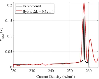
With the mechanism of the relationship betweenV_SMand differential resistance established, it is appropriate to consider a simplified approach to its calculation. The rate of change of current with respect to loss predicted by the DM model was found to vary slightly over the ranges of bias and loss investigated. Instead, a typical value of dI/dL=1.5×10−4kA/cm can be used in

conjunction with the experimentalI–V curve to calculateV_SMas

V_SM(I)= dVF R

dI (I)· dI dL

!

∆L, (7)

Current Density (A/cm

)

220

230

240

250

260

V

(V)

0

0.05

0.1

0.15

0.2

Experimental

Theory

∆

L= -0.3 cm

Theory

∆

L= -1.4 cm

Figure 3. Comparison of peak SM terminal voltage signal calculated with an inverse interpolation of the density matrix model output, and experimental SM measurement.

This hybrid approach requires a lower loss value (compared to the previous purely-theoretical approach) in order to achieve the same signal amplitude due to the effect of contact resistance. In the purely theoretical model, the contact resistance shifts the voltage to greater values. However this has no effect on the self-mixing signal since drive current is fixed, and the voltage change due to contact resistance is therefore constant. However, in Eq. (7) the differential resistance term contains this voltage shifting effect, and therefore predicts a larger self-mixing signal.

The value of dI/dLwill vary between different QCL devices depending mainly on the dipole matrix element of the upper-to-lower lasing level transition, doping density, and waveguide losses. This work suggests that QCLs that typically exhibit strong NDR regions, such as resonant LO phonon depopulated active regions may also exhibit sharpV_SMfeatures such as that observed in this work. For swept-frequency SM approaches [20] in which the QCL drive current is swept, the signal could in principle be improved over a wide range of biases by optimizing the differential resistance through modification of the QCL design.

6. Conclusion

Current Density (A/cm

)

220

230

240

250

260

V

(V)

0

0.05

0.1

0.15

0.2

Experimental

Hybrid

∆

L = 0.5 cm

Figure 4. Comparison of experimental and “hybrid”V_SMresults with a constant current–loss response of dI/dL=1.5 ×10−4kA/cm.

This model could be used to design and evaluate QCLs tailored to provide enhanced feedback effects at desired wavelengths.

Acknowledgements