Glacial geomorphological mapping: A review of
approaches and frameworks for best practice
CHANDLER, Benjamin M.P., LOVELL, Howard, BOSTON, Clare M., LUKAS,
Sven, BARR, Iestyn D., BENEDIKTSSON, Ivar O., BENN, Douglas I., CLARK,
ChrisD., DARVILL, Christopher M., EVANS, David J.A., EWERTOWSKI,
Marek W., LOIBL, David, MARGOLD, Martin, OTTO, Jan-Christoph,
ROBERTS, David H., STOKES, Chris R., STORRAR, Robert
<http://orcid.org/0000-0003-4738-0082> and STROEVEN, Arjen P.
Available from Sheffield Hallam University Research Archive (SHURA) at:
http://shura.shu.ac.uk/22264/
This document is the author deposited version. You are advised to consult the
publisher's version if you wish to cite from it.
Published version
CHANDLER, Benjamin M.P., LOVELL, Howard, BOSTON, Clare M., LUKAS, Sven,
BARR, Iestyn D., BENEDIKTSSON, Ivar O., BENN, Douglas I., CLARK, ChrisD.,
DARVILL, Christopher M., EVANS, David J.A., EWERTOWSKI, Marek W., LOIBL,
David, MARGOLD, Martin, OTTO, Jan-Christoph, ROBERTS, David H., STOKES,
Chris R., STORRAR, Robert and STROEVEN, Arjen P. (2018). Glacial
geomorphological mapping: A review of approaches and frameworks for best
practice. Earth-Science Reviews, 185, 806-846.
Copyright and re-use policy
See
http://shura.shu.ac.uk/information.html
Glacial geomorphological mapping:
1a review of approaches and frameworks for best practice
23
Benjamin M.P. Chandler1 *, Harold Lovell2, Clare M. Boston2, Sven Lukas3, Iestyn D. Barr4,
4
Ívar Örn Benediktsson5,Douglas I. Benn6, Chris D. Clark7, Christopher M. Darvill8,
5
David J.A. Evans9, Marek W. Ewertowski10, David Loibl11, Martin Margold12, Jan-Christoph Otto13,
6
David H. Roberts9, Chris R. Stokes9, Robert D. Storrar14, Arjen P. Stroeven15, 16
7 8
1 School of Geography, Queen Mary University of London, Mile End Road, London, E1 4NS, UK
9
2 Department of Geography, University of Portsmouth, Portsmouth, UK
10
3 Department of Geology, Lund University, Lund, Sweden
11
4 School of Science and the Environment, Manchester Metropolitan University, Manchester, UK
12
5 Institute of Earth Sciences, University of Iceland, Reykjavík, Iceland
13
6 Department of Geography and Sustainable Development, University of St Andrews, St Andrews, UK
14
7 Department of Geography, University of Sheffield, Sheffield, UK
15
8 Geography, School of Environment, Education and Development, University of Manchester, Manchester, UK
16
9 Department of Geography, Durham University, Durham, UK
17
10 Faculty of Geographical and Geological Sciences, Adam Mickiewicz University, Poznań, Poland
18
11 Department of Geography, Humboldt University of Berlin, Berlin, Germany
19
12 Department of Physical Geography and Geoecology, Charles University, Prague, Czech Republic
20
13 Department of Geography and Geology, University of Salzburg, Salzburg, Austria
21
14 Department of the Natural and Built Environment, Sheffield Hallam University, Sheffield, UK
22
15 Geomorphology & Glaciology,Department of Physical Geography, Stockholm University, Stockholm, Sweden
23
16 Bolin Centre for Climate Research, Stockholm University, Stockholm, Sweden
24 25
*Corresponding author. Email: [email protected] 26
27
Abstract
28 29
Geomorphological mapping is a well-established method for examining earth surface processes 30
and landscape evolution in a range of environmental contexts. In glacial research, it provides 31
crucial data for a wide range of process-oriented studies and palaeoglaciological 32
reconstructions; in the latter case providing an essential geomorphological framework for 33
establishing glacial chronologies. In recent decades, there have been significant developments 34
in remote sensing and Geographical Information Systems (GIS), with a plethora of high-quality 35
remotely-sensed datasets now (often freely) available. Most recently, the emergence of 36
unmanned aerial vehicle (UAV) technology has allowed sub-decimetre scale aerial images and 37
an important role in glacial geomorphology, particularly in cirque glacier, valley glacier and 39
icefield/ice-cap outlet settings. Field mapping is also used in ice sheet settings, but often takes 40
the form of necessarily highly-selective ground-truthing of remote mapping. Given the 41
increasing abundance of datasets and methods available for mapping, effective approaches are 42
necessary to enable assimilation of data and ensure robustness. This paper provides a review 43
and assessment of the various glacial geomorphological methods and datasets currently 44
available, with a focus on their applicability in particular glacial settings. We distinguish two 45
overarching ‘work streams’ that recognise the different approaches typically used in mapping 46
landforms produced by ice masses of different sizes: (i) mapping of ice sheet geomorphological 47
imprints using a combined remote sensing approach, with some field checking (where feasible); 48
and (ii) mapping of alpine and plateau-style ice mass (cirque glacier, valley glacier, icefield and 49
ice-cap) geomorphological imprints using remote sensing and considerable field mapping. Key 50
challenges to accurate and robust geomorphological mapping are highlighted, often 51
necessitating compromises and pragmatic solutions. The importance of combining multiple 52
datasets and/or mapping approaches is emphasised, akin to multi-proxy approaches used in 53
many Earth Science disciplines. Based on our review, we provide idealised frameworks and 54
general recommendations to ensure best practice in future studies and aid in accuracy 55
assessment, comparison, and integration of geomorphological data. These will be of particular 56
value where geomorphological data are incorporated in large compilations and subsequently 57
used for palaeoglaciological reconstructions. Finally, we stress that robust interpretations of 58
glacial landforms and landscapes invariably requires additional chronological and/or 59
sedimentological evidence, and that such data should ideally be collected as part of a holistic 60
assessment of the overall glacier system. 61
62
Keywords: glacial geomorphology; geomorphological mapping; GIS; remote sensing; field mapping 63
1. Introduction
76 77
1.1 Background and importance
78 79
Mapping the spatial distribution of landforms and features through remote sensing and/or field-based 80
approaches is a well-established method in Earth Sciences to examine earth surface processes and 81
landscape evolution (e.g. Kronberg, 1984; Hubbard and Glasser, 2005; Smith et al., 2011). Moreover, 82
geomorphological mapping is utilised in numerous applied settings, such as natural hazard 83
assessment, environmental planning, and civil engineering (e.g. Kienholz, 1977, Finke, 1980; Paron 84
and Claessens, 2011; Marc and Hovius, 2015; Griffiths and Martin, 2017). 85
86
Two overarching traditions exist in geomorphological mapping: Firstly, the classical approach 87
involves mapping all geomorphological features in multiple thematic layers (e.g. landforms, breaks of 88
slope, slope angles, and drainage), regardless of the range of different processes responsible for 89
forming the landscape. This approach to geomorphological mapping has been particularly widely used 90
in mainland Europe and has resulted in the creation of national legends to record holistic 91
geomorphological data that may be comparable across much larger areas or between studies (Demek, 92
1972; van Dorsser and Salomé, 1973; Leser and Stäblein, 1975; Klimaszewski, 1990; Schoeneich, 93
1993; Kneisel et al., 1998; Gustavsson et al., 2006; Rączkowska and Zwoliński, 2015). The second 94
approach involves more detailed, thematic geomorphological mapping commensurate with particular 95
research questions; for example, the map may have an emphasis on mass movements or glacial and 96
periglacial landforms and processes. Such a reductionist approach is helpful in ensuring a map is not 97
‘cluttered’ with less relevant data that may in turn make a multi-layered map unreadable (e.g. Kuhle, 98
1990; Robinson et al., 1995; Kraak and Ormeling, 2006). In recent years, the second approach has 99
become much more widespread due to increasing specialisation and thus forms the basis for this 100
review, which focuses on geomorphological mapping in glacial environments. 101
102
In glacial research, the production and analysis of geomorphological maps provide a wider context 103
and basis for various process-oriented and palaeoglaciological studies, including: 104
105
(1) analysing glacial sediments and producing process-form models (e.g. Price, 1970; Benn, 106
1994; Lukas, 2005; Benediktsson et al., 2016); 107
(2) quantitatively capturing the pattern and characteristics (‘metrics’) of landforms to understand 108
their formation and evolution (e.g. Spagnolo et al., 2014; Ojala et al., 2015; Ely et al., 2016a; 109
(3) devising glacial landsystem models that can be used to elucidate former glaciation styles or 111
inform engineering geology (e.g. Eyles, 1983; Evans et al., 1999; Evans, 2017; Bickerdike et 112
al., 2018); 113
(4) reconstructing the extent and dimensions of former or formerly more extensive ice masses 114
(e.g. Dyke and Prest, 1987a; Kleman et al., 1997; Houmark-Nielsen and Kjær, 2003; Benn 115
and Ballantyne, 2005; Glasser et al., 2008; Clark et al., 2012); 116
(5) elucidating glacier and ice sheet dynamics, including advance/retreat cycles, flow 117
patterns/velocities and thermal regime (e.g. Kjær et al., 2003; Kleman et al., 2008, 2010; 118
Evans, 2011; Boston, 2012a; Hughes et al., 2014; Darvill et al., 2017); 119
(6) identifying sampling locations for targeted numerical dating programmes and ensuring robust 120
chronological frameworks (e.g. Owen et al., 2005; Barrell et al., 2011, 2013; Garcia et al., 121
2012; Akçar et al., 2014; Kelley et al., 2014; Stroeven et al., 2014; Gribenski et al., 2016; 122
Blomdin et al., 2018); 123
(7) calculating palaeoclimatic variables for glaciated regions, namely palaeotemperature and 124
palaeoprecipitation (e.g. Kerschner et al., 2000; Bakke et al., 2005; Stansell et al., 2007; Mills 125
et al., 2012; Boston et al., 2015); and 126
(8) providing parameters to constrain and test numerical simulations of ice masses (e.g. Kleman 127
et al., 2002; Napieralski et al., 2007a; Golledge et al., 2008; Stokes and Tarasov, 2010; 128
Livingstone et al., 2015; Seguinot et al., 2016; Patton et al., 2017a). 129
130
Thus, accurate representation of glacial and associated landforms is crucial to producing 131
geomorphological maps of subsequent value in a wide range of glacial research. This is exemplified 132
in glacial geochronological investigations, where a targeted radiometric dating programme first 133
requires a clear geomorphological (and/or stratigraphic) framework and understanding of the 134
relationships and likely relative ages of different sediment-landform assemblages. In studies that 135
ignore this fundamental principle, it can be challenging to reconcile any scattered or anomalous 136
numerical ages with a realistic geomorphological interpretation, as the samples have been obtained 137
without a clear genetic understanding of the landforms being sampled (see Boston et al. (2015) and 138
Winkler (2018) for further discussion). 139
140
The analysis of geomorphological evidence has been employed in the study of glaciers and ice sheets 141
for over 150 years, with the techniques used in geomorphological mapping undergoing a number of 142
significant developments in that time. The earliest geomorphological investigations involved intensive 143
field surveys (e.g. Close, 1867; Penck and Brückner, 1901/1909; De Geer, 1910; Trotter, 1929; 144
Caldenius, 1932; Raistrick, 1933), before greater efficiency was achieved through the development of 145
aerial photograph interpretation from the late 1950s onwards (e.g. Lueder, 1959; Price, 1963; Welch, 146
Mollard and Janes, 1984). Satellite imagery and digital elevation models (DEMs) have been in 148
widespread usage since their development in the late 20th Century and have, in particular, helped
149
revolutionise our understanding of palaeo-ice sheets (e.g. Barents-Kara Ice Sheet: Winsborrow et al., 150
2010; British Ice Sheet: Hughes et al., 2014; Cordilleran Ice Sheet: Kleman et al., 2010; 151
Fennoscandian Ice Sheet: Stroeven et al., 2016; Laurentide Ice Sheet: Margold et al., 2018; 152
Patagonian Ice Sheet: Glasser et al., 2008). In recent times, increasingly higher-resolution DEMs have 153
become available due to the adoption of Light Detection and Ranging (LiDAR) technology (e.g. 154
Salcher et al., 2010; Jónsson et al., 2014; Miller et al., 2014; Dowling et al., 2015; Hardt et al., 2015; 155
Putniņš and Henriksen, 2017) and Unmanned Aerial Vehicles (UAVs) (e.g. Chandler et al., 2016a; 156
Evans et al., 2016a; Ewertowski et al., 2016; Tonkin et al., 2016; Ely et al., 2017). Aside from 157
improvements to remote sensing technologies, the last decade has seen a revolution in data 158
accessibility, with the proliferation of freely available imagery (e.g. Landsat data), freeware mapping 159
platforms (e.g. Google Earth) and open-source Geographical Information System (GIS) packages 160
(e.g. QGIS). As a result, tools for glacial geomorphological mapping are becoming increasingly 161
accessible, both practically and financially. 162
163
Field mapping remains a key component of the geomorphological mapping process, principally in the 164
context of manageable study areas relating to alpine- and plateau-style ice masses, i.e. cirque glaciers, 165
valley glaciers, icefields and ice-caps (e.g. Bendle and Glasser, 2012; Boston, 2012a, b; Jónsson et al., 166
2014; Gribenski et al., 2016; Lardeux et al., 2016; Brook and Kirkbride, 2018; Małecki et al., 2018). 167
This approach is also employed in ice sheet settings, but typically in the form of selective ground 168
checking of mapping from remotely-sensed data or focused mapping of regional sectors (e.g. Stokes 169
et al., 2013; Bendle et al., 2017a; Pearce et al., 2018). Frequently, field mapping is conducted in 170
tandem with sedimentological investigations (see Evans and Benn, 2004, for methods), providing a 171
means of testing preliminary interpretations and identifying problems for specific (and more detailed) 172
studies. This integrated approach is particularly powerful and enables robust interpretations of genetic 173
processes, glaciation styles and/or glacier dynamics (e.g. Benn and Lukas, 2006; Evans, 2010; 174
Benediktsson et al., 2010, 2016; Gribenski et al., 2016). In this context, it is worth highlighting the 175
frequent use of the term ‘sediment-landform assemblage’ (or ‘landform-sediment assemblage’) as 176
opposed to ‘landform’ in glacial geomorphology, underlining the importance of studying both surface 177
form and internal composition (e.g. Evans, 2003a, 2017; Benn and Evans, 2010; Lukas et al., 2017). 178
179
Geomorphological mapping using a combination of field mapping and remotely-sensed data 180
interpretation (hereafter ‘remote mapping’), or a number of remote sensing methods, permits a holistic 181
approach to mapping, wherein the advantages of each method/dataset can be combined to produce an 182
accurate map with robust genetic interpretations (e.g. Boston, 2012a, b; Darvill et al., 2014; Storrar 183
assimilation of data from these various sources, particularly where data are transferred from analogue 185
(e.g. hard-copy aerial photographs) to digital format. Apart from a few recent exceptions for specific 186
locations (e.g. the Scottish Highlands: Boston, 2012a, b; Pearce et al., 2014), there has been limited 187
explicit discussion of the approaches used to integrate geomorphological data in map production (i.e. 188
the relative contributions of different methods and/or datasets and their associated uncertainties), with 189
many contributions simply stating that the maps were produced through fieldwork and/or remote 190
sensing (e.g. Ballantyne, 1989; Lukas, 2007a; Evans et al., 2009a; McDougall, 2013). Given the 191
diversity of scales, data sources and research questions inherent in glacial geomorphological research, 192
and the increasing abundance of high-quality remotely-sensed datasets, finding the most cost- and 193
time- effective approach is difficult, especially for researchers new to the field. 194
195
1.2 Aims and scope
196 197
In this contribution, we review the wide range of approaches and datasets available to practitioners 198
and students for geomorphological mapping in glacial environments. The main aims of this review are 199
to (i) synthesise scale-appropriate mapping approaches that are relevant to particular glacial settings, 200
(ii) devise frameworks that will help ensure best practice when mapping, and (iii) encourage clear 201
communication of details on mapping methods used in glacial geomorphological studies. This will 202
ensure transparency and aid data transferability against a background of growing demand to collate 203
geomorphological (and chronological) data in regional compilations (e.g. the BRITICE project: Clark 204
et al., 2004, 2018a; the DATED-1 database: Hughes et al., 2016). A further aim of this contribution is 205
to emphasise the continued and future importance of field mapping in geomorphological research, 206
despite the advent of very high-resolution remotely-sensed datasets in recent years. 207
208
The following two sections of this review focus on field mapping (Section 2) and remote mapping 209
(Section 3), respectively. We consider these methods in a broadly chronological order to provide 210
historical context and illustrate the evolution of geomorphological mapping in glacial environments. 211
Section 4 discusses the errors associated with each mapping method, an important issue that often 212
receives limited attention within geomorphological studies. Within this discussion, we highlight 213
approaches that can help manage and minimise residual errors. Subsequently, we review the mapping 214
methods used in particular glacial environments (Section 5) and synthesise frameworks to help ensure 215
best practice when mapping (Section 6). 216
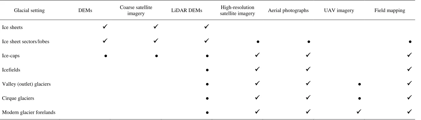
217
For the purposes of this review, we distinguish two overarching ‘work streams’: (i) mapping of 218
palaeo-ice sheet geomorphological imprints using a combined remote sensing approach, with some 219
field checking (where feasible); and (ii) mapping of alpine- and plateau-style ice mass 220
mapping/checking. The second workstream incorporates a spatial continuum of glacier morphologies, 222
namely cirque glaciers, valley glaciers, icefields and ice-caps (cf. Sugden and John, 1976; Benn and 223
Evans, 2010). The rationale for this subdivision is fourfold: Firstly, the approaches are governed by 224
the size of the (former) glacial systems and thus feasibility of using particular mapping methods in 225
certain settings (cf. Clark, 1997; Storrar et al., 2013). Secondly, there is a greater overlap of spatial 226
and temporal scales (i.e. more detailed records are preserved) in areas glaciated by smaller ice masses 227
that respond more rapidly to climate change (cf. Lukas, 2005, 2012; Bradwell et al., 2013; Boston et 228
al., 2015; Chandler et al., 2016b). Thirdly, the different mapping methodologies reflect the difficulties 229
in identifying vertical limits, thickness distribution and surface topography of palaeo-ice sheets (i.e. 230
emphasis often on mapping bed imprints) (cf. Stokes et al., 2015). Lastly, the overarching methods 231
employed to map glacial landforms in alpine and plateau settings do not differ fundamentally with ice 232
mass morphology, i.e. most studies in these environments employ a combination of field mapping and 233
remote sensing. In Section 5.3, we also specifically consider geomorphological mapping in modern 234
glacial environments to highlight important issues relating to the temporal resolution of remotely-235
sensed data and landform preservation potential. We emphasise the importance of utilising multiple 236
datasets and/or mapping approaches in an iterative process in all glacial settings (multiple remotely-237
sensed datasets in the case of ice-sheet-scale geomorphology) to increase accuracy and robustness, 238
akin to multi-proxy methodologies used in many Earth Science disciplines. 239
240
2. Field mapping methods
241 242
2.1 Background and applicability of field mapping
243 244
Traditionally, glacial geomorphological mapping has been undertaken through extensive field 245
surveys, an approach that dates back to the late 19th Century and early 20th Century (e.g. Close, 1867;
246
Goodchild, 1875; Partsch, 1894; Sollas, 1896; Penck and Brückner, 1901/1909; Kendall, 1902; 247
Wright, 1912; Hollingworth, 1931; Caldenius, 1932). Field mapping involves traversing the study 248
area and recording pertinent landforms onto (enlarged) topographic base maps (Figure 1). Typically, 249
field mapping is conducted at cartographic scales of ~1: 10,000 (e.g. Leser and Stäblein, 1975; Rupke 250
and De Jong, 1983; Thorp, 1986; Ballantyne, 1989; Evans, 1990; Benn et al., 1992; Mitchell and 251
Riley, 2006; Rose and Smith, 2008; Boston, 2012a, b) or 1: 25,000 (e.g. Leser, 1983; Ballantyne, 252
2002, 2007a, b; Benn and Ballantyne, 2005; Lukas and Lukas, 2006). Occasionally, it is conducted at 253
even larger scales, such as 1: 1,000 to 1: 5,000, but this is most appropriate for small areas or project-254
specific purposes (e.g. Kienholz, 1977; Leser, 1983; Lukas et al., 2005; Coray, 2007; Graf, 2007; 255
Reinardy et al., 2013). 256
With improvements in technology, the widespread availability of remotely-sensed datasets, and a 258
concomitant ease of access to high-quality printing facilities, alternative approaches to the traditional, 259
purely field mapping method have also been employed, including (i) documenting sediment-landform 260
assemblages during extensive field campaigns both prior to and after commencing remote mapping 261
(e.g. Dyke et al., 1992; Krüger 1994; Lukas and Lukas, 2006; Kjær et al. 2008; Boston, 2012a, b; 262
Jónsson et al., 2014; Schomacker et al. 2014; Everest et al., 2017), (ii) mapping directly onto or 263
annotating print-outs of imagery (e.g. aerial photographs) in the field (e.g. Lovell, 2014), (iii) 264
recording the locations of individual landforms using a (handheld) Global Navigation Satellite System 265
(GNSS) device (e.g. Bradwell et al., 2013; Brynjólfsson et al., 2014; Lovell, 2014; Małecki et al., 266
2018), or (iv) digitally mapping landforms in the field using a ruggedised tablet PC with built-in 267
GNSS and GIS software (e.g. Finlayson et al., 2011; Pearce et al., 2014). These approaches to field 268
mapping are particularly useful where large-scale topographic maps are unavailable or out of date. 269
270
Detailed field mapping is typically restricted to alpine- and plateau-style ice masses due to logistical 271
and financial constraints (Clark, 1997; Storrar et al., 2013). When conducted at the ice sheet scale, 272
field mapping is (or historically was) undertaken either as part of long-term campaigns by national 273
geological surveys in conjunction with surficial geology mapping programmes (e.g. Barrow et al., 274
1913; Flint et al., 1959; Krygowski, 1963; Campbell, 1967a, b; Hodgson et al., 1984; Klassen, 1993; 275
Priamonosov et al., 2000; Follestad and Bergstrøm, 2004) or necessarily highly-selective ground-276
truthing of remote mapping (e.g. Kleman et al., 1997, 2010; Golledge and Stoker, 2006; Stokes et al., 277
2013; Darvill et al., 2014; Stroeven et al., 2016; Pearce et al., 2018). 278
279
2.2 The field mapping process
280 281
Field mapping should ideally begin with systematic traverses of the study area – sometimes referred 282
to as a ‘walk-over’ (e.g. Demek, 1972; Otto and Smith, 2013) – to get a sense of the scale of the study 283
area and ensure that subtle features of importance, such as the location and orientation of ice-flow 284
directional indicators (e.g. flutes, striae, roches moutonnées and ice-moulded bedrock), are not 285
missed. In a palaeo-ice sheet context, mapping the location and orientation of striae in the field may 286
be of most interest as these can provide information on multiple (local) ice flow directions, of which 287
not all are recorded in the pattern of elongated bedforms (e.g. drumlins) mappable from remotely-288
sensed data (cf. Kleman, 1990; Hättestrand and Stroeven, 1996; Smith and Knight, 2011). Similarly, 289
in a contemporary outlet glacier context, flutes are an important indicator of ice flow direction – 290
sometimes of annual ice flow trajectories of glacier margins (cf. Chandler et al., 2016a; Evans et al., 291
2017) – but due to their subtlety they may only be identifiable in the field (e.g. Jónsson et al., 2014). 292
Traversing should ideally start from higher ground, where an overview can be gained, and proceed by 294
crossing a valley axis (or a cirque floor, for example) many times to enable the viewing and 295
assessment of landforms from as many perspectives, angles and directions as possible (cf. Demek, 296
1972). In addition to systematic traverses, landform assemblages in, for example, individual 297
valleys/basins should ideally be viewed from a high vantage point in low light (e.g. Benn, 1990). 298
Depending on the location and orientation of landforms, it may be beneficial to see the same area 299
either (i) early in the morning or late in the afternoon/evening due to longer shadows, or (ii) both in 300
the morning and afternoon/evening due to the changing position of longer shadows. These procedures 301
ensure that apparent dimensions and orientations, which are influenced by perception under different 302
viewing angles and daylight conditions, can be taken into account in descriptions and interpretations. 303
This approach circumvents potential complications relating to subtle features that may only be visible 304
from one direction or certain angles. 305
306
The location of features should be recorded on field maps or imagery (e.g. aerial photograph) extracts 307
with reference to ‘landmarks’ that are clearly identifiable both in the field and on the base 308
maps/imagery, such as distinct changes in contour-line inflection, lakes, river bends, confluences, 309
prominent bedrock exposures, and large ridges or mounds (Lukas and Lukas, 2006; Boston, 2012a, b). 310
Where geomorphological features are small, background relief is low and/or conspicuous reference 311
points are absent, a network of mapped reference points can be established by either taking a series of 312
cross-bearings on prominent features using a compass (e.g. Benn, 1990) or by verifying locations 313
using a handheld GNSS (e.g. Lukas and Lukas, 2006; Boston, 2012a, b; Brynjólfsson et al., 2014; 314
Jónsson et al. 2014; Lovell, 2014; Pearce et al., 2014; van der Bilt et al., 2016). The latter is useful for 315
recording the location of point-data such as striae, erratic or glacially-transported boulders, and 316
sediment exposures (cf. Lukas and Lukas, 2006; Boston, 2012a, b; Pearce et al., 2014). Additional 317
information between known reference points can then be interpolated and marked on the 318
geomorphological map. 319
320
Establishing the size of landforms and features and plotting them on the map as accurately as possible 321
is of crucial importance, and in addition to the inflections of contours (which may mark the location 322
and boundaries of prominent ridges, for example), the mapper may pace out and/or estimate lengths, 323
heights and widths. For larger landforms, or those masked by forest, walking around the perimeter of 324
landforms and establishing a GNSS-marked ‘waypoint-trail’ is a good first approximation. 325
326
The strategy outlined above offers a broad perspective on the overall landform pattern and ensures 327
accurate representation of landforms on field maps. To ensure accurate genetic interpretation of 328
individual landforms, and the landscape as a whole, this field mapping strategy should ideally form 329
331
2.3 Interpreting glacial landforms
332 333
In the preceding section, we focused on the technical aspects of field mapping and the means of 334
recording glacial landforms. However, geomorphological mapping typically forms the foundation of 335
process-oriented studies and palaeoglaciological reconstructions (see Section 1.1) and should, 336
therefore, be embedded within a process of observation and interpretation. Definitive interpretation of 337
glacial landforms, and glacial landscapes as a whole, can rarely be made on the basis of surface 338
morphology alone. Additional strands of field evidence may become highly relevant, if not essential, 339
depending on the objectives of the individual project: sedimentological data are crucial to interpreting 340
processes of landform formation and glacier dynamics (e.g. Lukas, 2005; Benn and Lukas, 2006; 341
Benediktsson et al., 2010, 2016; Chandler et al., 2016a; Gribenski et al., 2016), whilst chronological 342
data are fundamental to robust palaeoglaciological reconstructions and related palaeoclimatic studies 343
(e.g. Finlayson et al., 2011; Gribenski et al., 2016, 2018; Hughes et al., 2016; Stroeven et al., 2016; 344
Bendle et al., 2017b; Darvill et al., 2017). Moreover, time and resources are limited and pragmatism 345
necessary. Thus, observations must be targeted efficiently and effectively, in line with the research 346
aims. 347
348
Much field-based research adopts an inductive approach, in which observations are collected and used 349
to argue towards a particular conclusion. This is a valid approach at the exploratory stage of research, 350
but deeper understanding of a landscape requires a more iterative process, in which data collection is 351
conducted within a framework of hypothesis generation and testing. For this reason, it is useful to 352
adopt a number of alternative working hypotheses (Chamberlin, 1897) that can be tested and 353
gradually eliminated, following the principle of falsification (Popper, 1972). This process is best 354
conducted in the field when it is possible to make key observations to test an interpretation, especially 355
if the field site is remote and expensive to re-visit. 356
357
Following initial data collection, preliminary interpretations can be used to predict the outcome of 358
new observations, which can then be used to test and refine the interpretation. Well-framed 359
hypotheses allow an investigator to anticipate other characteristics of a glacial landscape and to test 360
those predictions by targeted investigation of key localities (see Benn, 2006). For example, the 361
presence of a certain group of landforms (e.g. moraines trending downslope into a side valley) can be 362
used to formulate hypotheses (e.g. blockage of the side-valley by glacier ice, and formation of a 363
glacial lake), which in turn can be used to predict the presence of other sediment-landform 364
associations in a particular locality (e.g. lacustrine sediments or shoreline terraces in the side-valley). 365
Further detailed geomorphological mapping (and sedimentological analyses) in that area would then 366
field mapping enable an increasingly detailed and robust understanding of the glacier system to be 368
constructed. This coupled inductive-deductive approach is much more powerful than a purely 369
inductive process: narratives that ‘explain’ a set of observations can appear very persuasive, even self-370
evident, but there may be other narratives that are also consistent with the same observations (cf. 371
Popper, 1972). 372
373
Process-form models are useful tools in this inductive-deductive approach to landscape interpretation. 374
In particular, landsystem or facies models make explicit links between landscape components and 375
genetic processes, providing structure and context for data collection and interpretation (e.g. Eyles, 376
1983; Brodzikowski and van Loon, 1991; Evans, 2003a; Benn and Evans, 2010). At best, process-377
form models are not rigid templates or preconceived categories into which observations are forced, 378
but a flexible set of possibilities that can guide, shape and enrich investigations (Benn and Lukas, 379
2006). For example, preliminary remote mapping may reveal features that suggest former glacier 380
lobes may have surged (e.g. Lovell et al., 2012). Systematic study of sediment-landform assemblages, 381
sediment exposures and other evidence, with reference to modern analogues (e.g. Evans and Rea, 382
2003), allows this idea to be rigorously evaluated in a holistic context (e.g. Darvill et al., 2017). This 383
can open up new avenues for research in a creative and open-ended process. 384
385
This inductive-deductive approach to interpreting glacial landscapes and events should be embedded 386
as part of the geomorphological mapping process (see Section 6). When dealing with palaeo-ice 387
sheets, such field-based investigations may be guided by (existing) remote mapping. In alpine and 388
plateau-style ice mass settings, sedimentological and chronological investigations should ideally form 389
an integral part of field surveys. 390
391
3. Remote mapping methods
392 393
In the following sections, we review the principal remote mapping approaches employed in glacial 394
geomorphological research, with analogue (or hard-copy) remote mapping (Section 3.1) and digital 395
remote mapping (Section 3.2) considered separately. We give an overview of a number of datasets 396
used for digital remote (i.e. GIS-based) mapping, namely satellite imagery (see Section 3.2.2.1), aerial 397
photographs (see Section 3.2.2.2), digital elevation models (see Section 3.2.2.3), freeware virtual 398
globes (see Section 3.2.2.4) and UAV-captured imagery (see Section 3.2.2.5). Each individual section 399
provides a brief outline of the historical background and development of the methods, and we discuss 400
the individual approaches in a broadly chronological order. Section 3.3 provides an overview of 401
image processing techniques, highlighting that pragmatic solutions are often required. 402
We focus principally on remotely-sensed datasets relevant to terrestrial (onshore) glacial settings in 404
the following sections because submarine (bathymetric) datasets and mapping of submarine glacial 405
landforms have been subject to recent reviews elsewhere (see Dowdeswell et al., 2016; Batchelor et 406
al., 2017). Nevertheless, we acknowledge that the emergence of geophysical techniques to investigate 407
submarine (offshore) glacial geomorphology is a major development over the last two decades. 408
Similarly, the emergence of geophysical datasets of sub-ice geomorphology in the last decade or so 409
has been revolutionary, particularly in relation to subglacial bedforms (see Stokes, 2018). Many of the 410
issues we discuss in relation to mapping from DEMs are transferable to those environments. 411
412
3.1 Analogue remote mapping
413 414
3.1.1 Background and applicability of analogue remote mapping
415
Geomorphological mapping from analogue (hard-copy) aerial photographs became a mainstream 416
approach in glacial geomorphology in the 1960s and 1970s, with early proponents including, for 417
example, the Geological Survey of Canada (e.g. Craig, 1961, 1964; Prest et al., 1968) and UK-based 418
researchers examining the Quaternary geomorphology of upland Britain (e.g. Price, 1961, 1963; 419
Sissons, 1967, 1977a, b, 1979a, b; Sugden, 1970) and contemporary glacial landsystems (e.g. Petrie 420
and Price, 1966; Price, 1966; Welch, 1966, 1967, 1968; Howarth, 1968; Howarth and Welch, 1969a, 421
b). The latter research on landsystems in Alaska and Iceland was particularly pioneering in that it 422
exploited a combination of aerial photograph interpretation, surveying techniques and early 423
photogrammetry (see Evans, 2009, for further details). 424
425
Despite continued development of remote sensing technologies and the availability of digital aerial 426
photographs (see Section 3.2.2.2), analogue stereoscopic aerial photographs are still used for glacial 427
geomorphological mapping (e.g. Hättestrand, 1998; Benn and Ballantyne, 2005; Lukas et al., 2005; 428
Hättestrand et al., 2007; Boston, 2012a, b; Evans and Orton, 2015). Additionally, the availability of 429
high-quality photogrammetric scanners means that archival, hard-copy aerial photographs can be 430
scanned at high resolutions, processed using digital photogrammetric methods and subsequently used 431
for on-screen vectorisation (Section 3.2; e.g. Bennett et al., 2010; Jónsson et al., 2014). 432
433
As with field mapping, the interpretation of analogue aerial photographs is primarily used for 434
mapping alpine- and plateau-style ice mass geomorphological imprints. Historically, analogue aerial 435
photograph interpretation was extensively used for mapping palaeo-ice sheet geomorphological 436
imprints, particularly by the Geological Survey of Canada, who combined aerial photograph 437
interpretation with detailed ground checking and helicopter-based surveys (e.g. Craig, 1961, 1964; 438
Hodgson et al., 1984; Aylsworth and Shilts, 1989; Dyke et al., 1992; Klassen, 1993; Dyke and 439
extensively to map glacial landforms relating to the Fennoscandian Ice Sheet (e.g. Sollid et al., 1973; 441
Kleman, 1992; Hättestrand, 1998; Hättestrand et al., 1999). Aerial photograph interpretation has 442
largely been superseded by satellite imagery and DEM interpretation in palaeo-ice sheet settings (see 443
Section 5.1) but is applied in palaeo-ice sheet contexts for more detailed mapping of selected and/or 444
complex areas (e.g. Dyke, 1990; Hättestrand and Clark, 2006; Kleman et al., 2010; Stokes et al., 445
2013; Storrar et al., 2013; Darvill et al., 2014; Evans et al., 2014). 446
447
3.1.2 Mapping from analogue datasets
448
For glacial geomorphological mapping purposes, vertical panchromatic aerial photographs have 449
traditionally been employed, with pairs of photographs (stereopairs) viewed in stereo using a 450
stereoscope (with magnification) (e.g. Karlén, 1973; Melander, 1975; Horsfield, 1983; Krüger, 1994; 451
Kleman et al., 1997; Hättestrand, 1998; Evans and Twigg, 2002; Jansson, 2003; Benn and Ballantyne, 452
2005; Lukas and Lukas, 2006; Boston, 2012a, b; Chandler and Lukas, 2017). During aerial surveys, 453
longitudinally-overlapping photographs along the flight path (endlap ≥ 60%) are captured in a series 454
of laterally-overlapping parallel strips (sidelap ≥ 30%), with the two different viewing angles of the 455
same area resulting in the stereoscopic effect (due to the principle of parallax; see Lillesand et al., 456
2015, for further details). This form of aerial photograph interpretation has been demonstrated to be a 457
particularly valuable tool for determining the exact location, shape and planform of small features in 458
glaciated terrain (e.g. Ballantyne, 1989, 2002, 2007a, b; Bickerton and Matthews, 1992, 1993; Lukas 459
and Lukas, 2006; Boston, 2012a, b), provided the photographs are of appropriate scale, quality and 460
tonal contrast (cf. Benn, 1990; Benn et al., 1992). 461
462
Mapping from hard-copy aerial photographs is undertaken by drawing onto acetate sheets 463
(transparency films) whilst viewing the aerial photographs through a stereoscope, with the acetate 464
overlain on one photograph of a stereopair (Figure 2). Ideally, mapping should be conducted using a 465
super-fine pigment liner with a nib size of 0.05 mm to enable small features to be mapped. Even so, it 466
may still be necessary to compromise on the level of detail mapped; for example, meltwater channels 467
between ice-marginal moraines have been left off maps in some studies due to map scale, with the 468
associated text describing chains of moraines interspersed with meltwater channels (e.g. Benn and 469
Ballantyne, 2005; Lukas, 2005). 470
471
Examining stereopairs from multiple sorties (‘flight missions’) in parallel or in combination with 472
digital aerial photographs may be beneficial and help alleviate issues such as localised cloud cover, 473
snow cover, poor tonal contrast, afforestation, and anthropogenic developments (e.g. Horsfield, 1983; 474
Bennett, 1991; McDougall, 2001). Additionally, it is advantageous to examine stereopairs multiple 475
times – preferably before and after field mapping – to increase feature identification and improve the 476
conducting mapping over a large area with multiple stereopairs, examining stereopairs from a sortie 478
‘out of sequence’ (i.e. not mapping from consecutive pairs of photographs) may provide a means of 479
internal corroboration and ensure objectivity and robustness (Bennett, 1991). 480
481
In order to reduce geometric distortion, which increases towards the edges of aerial photographs due 482
to the central perspective (Lillesand et al., 2015), it is advisable to keep the areas mapped onto the 483
acetate as close as possible to the centre of one aerial photograph of a stereopair (Kronberg, 1984; 484
Lukas, 2002, 2005a; Evans and Orton, 2015). These hand-drawn overlays can subsequently be 485
scanned at high resolutions and then georeferenced and vectorised using GIS software (see Section 486
3.3.1). 487
488
3.2 Digital remote mapping
489 490
3.2.1 Background and applicability of digital remote mapping
491
The development of GIS software packages (e.g. commercial: ArcGIS; open source: QGIS) and the 492
proliferation of digital imagery, particularly freely available satellite imagery, have undoubtedly been 493
the most significant developments in glacial geomorphological mapping in the last fifteen years or so. 494
GIS packages have provided platforms and tools for visualising, maintaining, manipulating and 495
analysing vast quantities of remotely-sensed and geomorphological data (cf. Gustavsson et al., 2006, 496
2008; Napieralski et al., 2007b). Their use in combination with digital imagery allows 497
geomorphological features to be mapped directly in GIS software (Figure 3), with individual vector 498
layers created for each geomorphological feature. Moreover, the availability of digital imagery 499
enables the mapper to alter the viewing scale instantaneously and switch between various 500
datasets/types, allowing for a flexible but systematic approach. 501
502
Digital mapping (on-screen vectorisation/tracing) also provides georeferenced geomorphological data, 503
which has two important benefits: Firstly, these data can easily be used to extract landform metrics 504
(e.g. Hättestrand et al., 2004; Clark et al., 2009; Spagnolo et al., 2010, 2014; Storrar et al., 2014; Ojala 505
et al., 2015; Dowling et al., 2016; Ely et al., 2016a, 2017a); and, secondly, these data can be 506
seamlessly incorporated into wider, regional-scale GIS compilations (e.g. Bickerdike et al., 2016; 507
Stroeven et al., 2016; Clark et al., 2018a). Additionally, digital remote mapping allows the user to 508
record attribute data (e.g. data source) tied to individual map (vector) layers, which can be useful for 509
large compilations of previously published mapping (e.g. Bickerdike et al., 2016; Clark et al., 2018a). 510
Such compendia help to circumvent issues relating to the often-fragmented nature of 511
geomorphological evidence (i.e. numerous spatially separate studies) and identify gaps in the mapping 512
record. Once assembled across large areas, they also enable evidence-based reconstructions of entire 513
access data revolution in academia and the increasing publication/availability of mapping output (in 515
the form of GIS files; e.g. Finlayson et al., 2011; Fu et al., 2012; Darvill et al., 2014; Bickerdike et al., 516
2016; Bendle et al., 2017a), means that geomorphological mapping can have wider impact beyond 517
individual local to regional studies. 518
519
3.2.2 Datasets for digital remote mapping
520
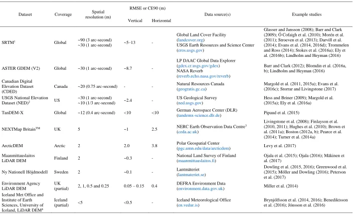
There is now a plethora of remotely-sensed datasets covering a wide range of horizontal resolutions 521
(10-2 to 102 m), enabling the application of digital mapping (in some form) to all glacial settings. We
522
provide an overview of the principal datasets used in digital mapping below, with mapping 523
approaches in specific glacial settings reviewed in Section 5. 524
525
3.2.2.1 Satellite imagery. The development of satellite-based remote sensing in the 1970s and 526
subsequent advances in technology have revolutionised understanding of glaciated terrain, particularly 527
with respect to palaeo-ice sheet geomorphology and dynamics (see Section 5.1; Clark, 1997; Stokes, 528
2002; Stokes et al., 2015). The potential of satellite imagery was first demonstrated by the pioneering 529
work of Sugden (1978), Andrews and Miller (1979) and Punkari (1980), with the availability of large-530
area view (185 km x 185 km) Landsat Multi-Spectral Scanner (MSS) images affording a new 531
perspective of glaciated regions. These allowed a single analyst to systematically map ice-sheet-scale 532
(1:45,000 to 1: 1,000,000) glacial geomorphology (e.g. Boulton and Clark, 1990a, b) in a way that 533
previously would have required the painstaking mosaicking of thousands of aerial photographs (e.g. 534
Prest et al., 1968). 535
536
Since the 1980s, there has been an explosion in the use of satellite imagery for glacial 537
geomorphological mapping and there is now a profusion of datasets available (Table 1). Importantly, 538
many of these sensors capture multispectral data, which can enhance landform detection through 539
image processing and the use of different band combinations (see Section 3.3.2). The uptake of 540
satellite imagery has coincided with improvements in the availability and spatial and spectral 541
resolution of satellite datasets globally, with Landsat (multispectral: 30 m; panchromatic: 15 m), 542
ASTER (15 m), Sentinel-2 (10 m) and SPOT (up to 1.5 m) images proving the most popular. More 543
recently, satellite sensor advancements have enabled the capture of satellite images with resolutions 544
comparable to aerial photographs (Figure 4; e.g. QuickBird, SPOT6-7, WorldView-2 and later). These 545
datasets are also suitable for mapping typically smaller and/or complex glacial landforms produced by 546
cirque glaciers, valley glaciers and icefield/ice-cap outlets (e.g. Chandler et al., 2016a; Evans et al., 547
2016b; Ewertowski et al., 2016; Gribenski et al., 2016; Małecki et al., 2018). 548
549
In general, as better-resolution imagery has become more widely available at low to no cost, older, 550
Landsat data (TM, ETM+, and OLI: 15 to 30 m) are still the standard data source for ice-sheet-scale 552
mapping, with the uptake of high-resolution commercial satellite imagery still relatively slow in such 553
studies. This is primarily driven by the cost of purchasing high-resolution commercial datasets, 554
making freely-available imagery such as Landsat a valuable resource. In addition, archival satellite 555
data afford time-series of multi-spectral images that may facilitate assessments of geomorphological 556
changes through time; for example, fluctuations in highly dynamic (surging or rapidly retreating) 557
glacial systems (e.g. Flink et al., 2015; Jamieson et al., 2015). Conversely, for smaller research areas 558
(e.g. for a single valley or foreland), high-resolution satellite imagery is becoming an increasingly 559
viable option, with prices for georeferenced and orthorectified products comparable to those for 560
digital aerial photographs (see Section 3.2.2.2). This also has the benefit of saving time on 561
photogrammetric processing, with many vendors providing consumers with various processing 562
options. Consequently, on-demand, high-resolution (commercial) satellite imagery will inevitably 563
come into widespread usage, where costs are not prohibitive. Alternatively, freeware virtual globes 564
and web mapping services (e.g. Bing Maps, Google Earth) offer valuable resources for free 565
visualisation of such high-resolution imagery (see Section 3.2.2.4). 566
567
3.2.2.2 Digital aerial photographs. With improvements in technology, high-resolution (ground 568
resolution <0.5 m per pixel) digital copies of aerial photographs have become widely available and 569
used for glacial geomorphological mapping (e.g. Brown et al., 2011a; Bradwell et al., 2013; 570
Brynjólfsson et al., 2014; Jónsson et al., 2014; Pearce et al., 2014; Schomacker et al., 2014; Chandler 571
et al., 2016a; Evans et al., 2016c; Lardeux et al., 2016; Lønne, 2016; Allaart et al., 2018). Indeed, 572
digital aerial photographs, along with scanned copies of archival aerial photographs, are now more 573
widely used than hard-copy stereoscopic aerial photographs, particularly in modern glacial settings. 574
Additionally, the introduction of UAV technology in recent years has allowed sub-decimetre 575
resolution aerial photographs to be captured on demand (see Section 3.2.2.5). A further key advantage 576
of aerial photographs in digital format is the ability to produce orthorectified aerial photograph 577
mosaics (or ‘orthophotographs’) and DEMs with low root mean square errors (RMSEs <1 m; see 578
Section 4.4), when combined with ground control points (GCPs) collected using surveying equipment 579
(e.g. Kjær et al. 2008; Bennett et al., 2010; Schomacker et al., 2014; Chandler et al., 2016b; Evans et 580
al., 2017). These photogrammetric products can then be used for on-screen vectorisation (tracing) and 581
the generation of georeferenced geomorphological mapping (Figure 5), as outlined above. 582
583
Digital aerial photographs are commonly captured by commercial surveying companies (e.g. 584
Loftmyndir ehf, Iceland; Getmapping, UK), meaning that they may be expensive to purchase and 585
costs may be prohibitive for large study areas. This is in contrast to hard-copy (archival) aerial 586
photographs that are often freely available for viewing in national collections. Additionally, digital 587
screen mapping in stereoscopic view is possible on workstations equipped with stereo display and 589
software such as BAE Systems SOCET SET (e.g. Kjær et al., 2008; Benediktsson et al., 2009). 590
However, this approach is not applicable to orthophotographs. An alternative approach is to visualise 591
orthophotographs in 3D by draping them over a DEM (see Section 3.2.2.3) in GIS software such as 592
ESRI ArcScene or similar (Figure 6; e.g. Benediktsson et al., 2010; Jónsson et al., 2014; Schomacker 593
et al., 2014; van der Bilt et al., 2016). Three-dimensional assessment in ArcScene,parallel to mapping 594
in ArcMap, may aid in landform detection, delineation and interpretation. 595
596
3.2.2.3 Digital Elevation Models (DEMs). Over the last ~15 years there has been increasing use of 597
DEMs in glacial geomorphology, particularly for mapping at the ice sheet scale (e.g. Glasser and 598
Jansson, 2008; Hughes et al., 2010; Ó Cofaigh et al., 2010; Evans et al., 2014, 2016d; Ojala, 2016; 599
Principato et al., 2016; Stokes et al., 2016a; Mäkinen et al., 2017; Norris et al., 2017). DEMs are 600
raster-based models of topography that record absolute elevation, with each grid cell in a DEM 601
representing the average height for the area it covers (Clark, 1997; Smith et al., 2006). Terrestrial 602
DEMs can be generated by a variety of means, including from surveyed contour data, directly from 603
stereo imagery (aerial photographs, satellite and UAV-captured imagery), or from air- and space-604
borne radar and LiDAR systems (Smith and Clark, 2005). An important recent development in this 605
regard has been the ‘Surface Extraction with TIN-based Search-space Minimization’ (SETSM) 606
algorithm for automated extraction of DEMs from stereo satellite imagery (Noh and Howat, 2015), 607
which has been used to generate the ArcticDEM dataset (https://www.pgc.umn.edu/data/arcticdem/). 608
However, SETSM DEMs may contain systematic vertical errors that require correction (e.g. Carrivick 609
et al., 2017; Storrar et al., 2017). 610
611
The majority of DEMs with national- to international-scale coverage (Table 2) typically have a 612
coarser spatial resolution than aerial photographs and satellite imagery and represent surface 613
elevations rather than surface reflectance. As a result, it may be difficult to identify glacial landforms 614
produced by relatively small ice masses (cirque glaciers, valley glaciers and icefield outlets), 615
precluding detailed mapping of their planforms (cf. Smith et al., 2006; Hughes et al., 2010; Brown et 616
al., 2011a; Boston, 2012a, b; Pearce et al., 2014). Conversely, these DEMs can be particularly 617
valuable for mapping glacial erosional features (e.g. glacial valleys, meltwater channels), as well as 618
major glacial depositional landforms produced by larger ice masses (e.g. Greenwood and Clark, 2008; 619
Heyman et al., 2008; Livingstone et al., 2008; Hughes et al., 2010; Morén et al., 2011; Barr and Clark, 620
2012; Stroeven et al., 2013; Turner et al., 2014a; Margold et al., 2015a; Blomdin et al., 2016a, b; 621
Lindholm and Heyman, 2016; Mäkinen et al., 2017; Storrar and Livingstone, 2017). However, the 622
recent development of UAV (see section 3.2.2.5) and LiDAR technologies have allowed the 623
generation of very high resolution DEMs (<0.1 m), enabling the application of DEMs to map small 624
national-scale LiDAR DEMs becoming widely-used in the future, with a number of nations recently 626
releasing or currently capturing/processing high horizontal resolution (≤2 m) LiDAR data (Table 2; 627
e.g. Dowling et al. 2013; Johnson et al. 2015). 628
629
Although the principal focus of this contribution is terrestrial/onshore glacial geomorphological 630
mapping, it is worth highlighting here that the availability of spatially-extensive bathymetric charts, 631
such as the General Bathymetric Chart of the Oceans (GEBCO) and International Bathymetric Chart 632
of the Arctic Ocean (IBCAO: Jakobsson et al., 2012), and high-resolution, regional (often industry-633
acquired) bathymetric data has been an important development in submarine/offshore glacial 634
geomorphological mapping. This has enabled the gridding of DEMs to map submarine glacial 635
geomorphological imprints (see Dowdeswell et al., 2016), markedly enhancing understanding of 636
palaeo-ice sheets in marine sectors (e.g. Ottesen et al., 2005, 2008a, 2016; Bradwell et al., 2008; 637
Winsborrow et al., 2010, 2012; Livingstone et al., 2012; Ó Cofaigh et al., 2013; Hodgson et al., 2014; 638
Stokes et al., 2014; Margold et al., 2015a, b; Greenwood et al., 2017) and modern tidewater (often 639
surging) glaciers (e.g. Ottesen and Dowdeswell, 2006; Ottesen et al., 2008b, 2017; Robinson and 640
Dowdeswell, 2011; Dowdeswell and Vazquez, 2013; Flink et al., 2015; Streuff et al., 2015; Allaart et 641
al., 2018). In addition, recent years have seen the production of DEMs of sub-ice topography from 642
geophysical datasets (radar and seismics) at spatial resolutions suitable for identifying and mapping 643
bedforms (see King et al., 2007, 2009, 2016a; Smith et al., 2007; Smith and Murray, 2009). This work 644
has advanced understanding of the evolution of bedforms beneath Antarctic ice streams, providing 645
important genetic links between the formation of landforms beneath modern ice sheets and those left-646
behind by palaeo-ice masses (Stokes, 2018). The interested reader is directed to recent reviews for 647
further discussion on the importance of geophysical evidence for understanding ice sheet extent and 648
dynamics (Livingstone et al., 2012; Ó Cofaigh, 2012; Stokes et al., 2015; Dowdeswell et al., 2016; 649
Batchelor and Dowdeswell, 2017; Stokes, 2018). 650
651
3.2.2.4 Freeware virtual globes. The advent of freeware virtual globes (e.g. Google Earth, NASA
652
Worldwind) and web mapping services (e.g. Bing Maps, Google Earth Engine, Google Maps) has 653
provided platforms for free visualisation of imagery from various sources and low-cost mapping 654
resources. A key benefit of virtual globes is the ability to visualise imagery and terrain in 3D and from 655
multiple viewing angles, which may aid landform detection when used in conjunction with other 656
datasets and software (e.g. Heyman et al., 2008; Bendle et al., 2017a). Moreover, a number of virtual 657
globes and web mapping services have the ability to link with other freeware and open-source 658
programmes; for example, free plugins are available to import Google Earth and Bing Maps imagery 659
into the open-source GIS software package QGIS. Thus, a mapper can combine freely available, often 660
GIS technology without the expense associated with commercial imagery and software (see Sections 662
3.2.2.1 and 3.2.2.2). 663
664
The most widely-used virtual globe is Google Earth, with a ‘professional’ version (Google Earth Pro) 665
freely available since 2015 (see Mather et al., 2015, for a review). An increasing number of glacial 666
geomorphological studies are noting the use of Google Earth (but not necessarily the imagery type) as 667
a mapping tool (see Table 1), principally to cross-check mapping conducted from other imagery. 668
However, some studies have also utilised the built-in vectorising tools for mapping (e.g. Margold and 669
Jansson, 2011; Margold et al., 2011; Fu et al., 2012). There is a compromise on the functionality of 670
freeware virtual globes and vectorisation tools are often not as flexible and/or user-friendly, but these 671
can be overcome by importing imagery into GIS software. In the case of Google Earth, it is also 672
possible to export Keyhole Markup Language (KML) files that can be used for subsequent analyses 673
and map production in GIS software (following file conversion). Open access remotely-sensed 674
datasets are also available through commercial GIS software, with high resolution satellite imagery 675
(e.g. GeoEye-1, SPOT-5, WorldView) available for mapping through the in-built ‘World Imagery’ 676
service in ESRI ArcGIS (e.g. Bendle et al., 2017a). 677
678
Despite the benefits, some caution is necessary when using freeware virtual globes as there may be 679
substantial errors in georeferencing of imagery, which users cannot account for and/or correct. 680
Moreover, dating of imagery is not necessarily clear or accurate (Mather et al., 2015; Wyshnytzky, 681
2017). The latter may not be a concern if mapping in a palaeoglaciological setting, whilst any 682
georeferencing errors may not be as significant if mapping broad patterns at the ice sheet scale. 683
Conversely, errors associated with freeware mapping may be significant when comparing imagery 684
from different times and/or when mapping in highly dynamic, contemporary glacial environments. 685
Aside from these potential issues, limitations are imposed by pre-processing of imagery, with no 686
option to, for example, modify band combinations to enhance landform detection (see Section 3.3.2). 687
688
3.2.2.5 UAV-captured imagery. The recent emergence of UAV technology provides an alternative 689
method for the acquisition of very high-resolution (<0.1 m per pixel) geospatial data that circumvents 690
some of the issues associated with more established approaches, particularly in relation to temporal 691
resolution and the high-cost of acquiring commercial remotely-sensed data (see also Smith et al., 692
2016a). Following the initial acquisition of the UAV and associated software, this method provides a 693
rapid, flexible and relatively inexpensive means of acquiring up-to-date imagery at an unprecedented 694
spatial resolution and it is becoming increasingly employed in glacial research (Figure 7; Rippin et al., 695
2015; Ryan et al., 2015; Chandler et al., 2016b; Ewertowski et al., 2016; Tonkin et al., 2016; Westoby 696
et al., 2016; Ely et al., 2017; Allaart et al., 2018). UAV-captured images are processed using 697
common software in use at present (e.g. Chandler et al., 2016b; Evans et al., 2016a; Ely et al., 2017; 699
Allaart et al., 2018). This methodology has enabled the production of sub-decimetre resolution 700
orthophotographs and DEMs with centimetre-scale error values (RMSEs <0.1 m; see Section 4.4) for 701
glacial geomorphological mapping (e.g. Evans et al., 2016a; Ely et al., 2017). Although surveying of 702
GCPs is still preferable for processing UAV-captured imagery, a direct georeferencing workflow (see 703
Turner et al., 2014b, for further details) is capable of producing reliable geospatial datasets from 704
imagery captured using consumer-grade UAVs and cameras, without the need for expensive survey 705
equipment (see Carbonneau and Dietrich, 2017). 706
707
The use of UAVs will be valuable in future glacial geomorphological research due to their flexibility 708
and low-cost. In particular, UAVs open up the exciting possibility of undertaking repeat surveys at 709
high temporal (sub-annual to annual) resolutions in modern glacial settings (Immerzeel et al., 2014; 710
Chandler et al., 2016b; Ely et al., 2017). Multi-temporal UAV imagery will enable innovative 711
geomorphological studies on issues such as (i) the modification and preservation potential of 712
landforms over short timescales (Ely et al., 2017), (ii) the frequency of ice-marginal landform 713
formation, particularly debates on sub-annual to annual landform formation (Chandler et al., 2016b), 714
and (iii) changes in process-form regimes at contemporary ice-margins (Evans et al., 2016a). 715
716
Using UAVs to capture aerial imagery is not without challenges, particularly in relation to the 717
challenge of intersecting suitable weather conditions in modern glacial environments: many UAVs are 718
unable to fly in high windspeeds, whilst rain can infiltrate electrical components and create hazy 719
imagery (Ely et al., 2017). Flight times and areal coverage are also limited by battery life, with some 720
battery packs permitting as little as 10 minutes per flight. There are also legal considerations, with the 721
use of UAVs prohibited in some localities/countries or requiring licenses/permits. Moreover, there 722
may be restrictions on flying heights and UAVs may need to be flown in visual line of sight, further 723
limiting areal coverage. Nevertheless, we envisage UAV technology becoming more widespread and 724
a key tool in high-resolution glacial geomorphological investigations, especially if future 725
technological developments can increase the range of conditions in which UAVs can be flown. In 726
future, it is likely that UAV technology will be primarily used for investigating short-term changes 727
across relatively small areas. 728
729
3.3 Image processing for mapping
730 731
An important part of geomorphological mapping is processing remotely-sensed datasets in preparation 732
for mapping, but this is often given limited prominence in glacial geomorphological studies. 733
Crucially, processing of remotely-sensed data aids the identification of glacial landforms and ensures 734