Neural network approach to modeling liquid crystals in complex confinement

(1)

Neural-network approach to modeling liquid crystals in

complex confinement

SANTOS-SILVA, T, TEIXEIRA, P.I.C., ANQUETIL-DECK, C. and CLEAVER,

Doug <http://orcid.org/0000-0002-4278-0098>

Available from Sheffield Hallam University Research Archive (SHURA) at:

http://shura.shu.ac.uk/8170/

This document is the author deposited version. You are advised to consult the publisher's version if you wish to cite from it.

Published version

SANTOS-SILVA, T, TEIXEIRA, P.I.C., ANQUETIL-DECK, C. and CLEAVER, Doug (2014). Neural-network approach to modeling liquid crystals in complex confinement. Physical Review E, 89 (5), 053316.

Copyright and re-use policy

See http://shura.shu.ac.uk/information.html

(2)

A neural network approach to modelling liquid crystals

in complex confinement

T. Santos-Silva1_{, P. I. C. Teixeira}2,3_{, C. Anquetil-Deck}4∗ _{and D. J. Cleaver}4 1_{Faculdade de Engenharia, Universidade Cat´}_{olica Portuguesa}

Estrada de Tala´ıde, P-2635-631 Rio de Mouro, Portugal

2_{Instituto Superior de Engenharia de Lisboa}

Rua Conselheiro Em´ıdio Navarro 1, P-1950-062 Lisbon, Portugal

3_{Centro de F´ısica Te´}_{orica e Computacional}

Faculdade de Ciˆencias, Universidade de Lisboa

Avenida Professor Gama Pinto 2, P-1649-003 Lisbon, Portugal

4_{Materials and Engineering Research Institute, Sheffield Hallam University}

Pond Street, Sheffield S1 1WB, United Kingdom

(3)

Abstract

Finding the structure of a confined liquid crystal is a difficult task since both the density and

order parameter profiles are non-uniform. Starting from a microscopic model and density-functional

theory, one has to either (i) solve a non-linear, integral Euler-Lagrange equation, or (ii) perform

a direct multi-dimensional free energy minimisation. The traditional implementations of both

approaches are computationally expensive and plagued with convergence problems. Here, as an

alternative, we introduce an unsupervised variant of the Multi-Layer Perceptron (MLP) artificial neural network for minimising the free energy of a fluid of hard non-spherical particles confined

between planar substrates of variable penetrability. We then test our algorithm by comparing

its results for the structure (density-orientation profiles) and equilibrium free energy with those

obtained by standard iterative solution of the Euler-Lagrange equations and with Monte Carlo

simulation results. Very good agreement is found and the MLP method proves competitively

fast, flexible and refinable. Furthermore, it can be readily generalised to the richer experimental

patterned-substrate geometries that are now experimentally realisable but very problematic to

conventional theoretical treatments.

PACS numbers: 68.08.-p, 64.70.mf, 61.30.Hn

∗_{Present address: Karlsruhe Institute of Technology, Institute for Meteorology and Climate Research,}

Atmo-spheric Aerosol Research Department (IMK-AAF), Hermann-von-Helmholtz-Platz 1, D-76344

(4)

I. INTRODUCTION

In a world suffused with images, displays are paramount. Of these, liquid crystal (LC) devices (LCDs) have a huge market share [1]. LCs are a state of matter intermediate between solid and liquid; they retain some of the order of a solid, but are free to flow as a liquid [2]. In particular, their constituent particles, which are typically elongated, all point, on average, in the same direction, termed the director; the extent of this alignment is given by the LC order parameter.

The director orientation is determined by effects external to the LC itself. All current LCDs are basically light valves that rely, for their operation, on the competing actions of bounding surfaces – known as anchoring – and applied fields on the director (see, e.g., [3, 4]). Typically an LC layer is sandwiched between suitably prepared substrates, which may favour the same (symmetric) or different (hybrid) alignments. An electric field is then used to deviate the orientational order profile from that induced by the substrates alone. Two examples are the conventional (and highly successful) twisted-nematic (TN) cell [4] found in most TV screens, and the more recent hybrid aligned nematic (HAN) cell of Bryan-Brown

et al. [5, 6]. The latter has led to a practical realisation of a bistabledevice: unlike the TN cell, a bistable device has two optically distinct, stable states and an applied voltage is only needed when switching between them, with consequent substantial energy savings.

Applications of LCDs beyond displays include sensors. For example, it has been shown that a LC film deposited at the air-water interface can be switched in and out of the HAN state by varying the surfactant concentration in the water, thereby providing an easy-to-read surfactant detector [7]. LC confinement is also pertinent to some of the many fascinating LC colloid systems devised in recent years [8], where the LC matrix is squeezed to microscopic dimensions when the colloidal particles self-aggregate.

(5)

non-uniform, the free energy is a functional of the density-orientation profile – i.e., it depends on the density, director and order parameter at each point in the region occupied by the LC – and minimisation is difficult. Two major routes are then possible: (i) functionally to differentiate the free energy and thereby derive a non-linear, integral Euler-Lagrange (EL) equation, which must then be solved; or (ii) to perform a direct multi-dimensional free energy minimisation. Route (i), essentially in the form of Picard iteration [9], has been used by many workers including ourselves [10, 11]; it is easier to implement, but may fail to converge, converge very slowly,or converge to a local minimum, especially if the density-orientation profile is strongly non-uniform and the initial guess is not carefully made. Route (ii) basically uses variants of the conjugate-gradient scheme [12, 13]; it is more reliable, less dependent on the quality of the initial guess, and possibly somewhat faster, but harder to implement.

To our knowledge, only systems that exhibit spatial variability along one dimension have been investigated by microscopic theory. Whereas this comprises the most popular device geometries including the TN and hybrid HAN cells, it is now possible to pattern substrates along either one or two dimensions, and thereby create novel, more versatile aligning layers for LCs [14–17]. Various of these complex substrates have found application in bistable LCDs such as the zenithally bistable nematic [6], post-aligned bistable nematic [18] and square well array [19, 20] devices. If one wishes to study these using the microscopic theorist’s premiyer formalism, functional theory (DFT), one ends up needing to represent the density-orientation profile – which is a function of at least two angles, in addition to the spatial coordinates – on a very large grid of points. Moreover, the interactions between any two particles at any positions and with any orientations, need to be specified by a potentially huge interaction kernel, computation of which requires very fast processors and/or very large RAM. Ideally one would like to have a toolbox that would permit fast, accurate and reliable calculation of the structure of a LC layer confined between substrates of many different patterns, in either symmetric or hybrid combinations. This would help guide researchers as to what configurations might be more promising for applications without actually having to manufacture them – the latter is a laborious and often expensive endeavour.

(6)

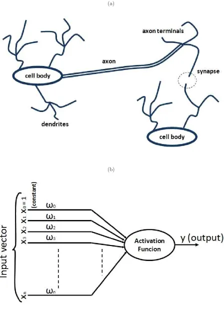
one that, to our knowledge, has not yet been exploited in the context of LC modelling is artificial neural networks (ANN). ANNs are a class of learn-by-example systems that have some features in common with biological neurones [21]. Biological neurones fire (or not) depending on the input (usually neurotransmitters) they receive (see figure 1). Some ANNs mimic this behaviour by making artificial units compute an affine transformation for their input vector, followed by some monotonic activation function.

The main difficulty in solving a particular problem is representation, i.e., designing a neural network that is rich enough that its output is able to reproduce a function of the required complexity. In fact, in general the representation of the solution is itself a con-straint. In this paper, we describe an approach to learning the density-orientation profile of a confined LC within the framework of an ANN. We focus on a particular type of ANN – the Multilayer Perceptron (MLP) – which has been shown to be a universal approximator for all Borel-measurable functions [22]. This makes the MLP a good candidate for tackling the representation problem. Furthermore, the MLP is a well-studied learning system, for which many algorithms have been developed to speed up convergence. This paper does not concern the use of acceleration algorithms: rather, its main aim is to determine whether MLP networks are applicable to, and may offer an alternative way of addressing the problem of,calculating the structure of a confined LC. This requires modifying the MLP to perform

unsupervised learning, as the value of the equilibrium free energy is not known a priori. We do not claim that the MLP we developed is the best method for any one particular application – our aim was just to add another tool to the theorist’s toolbox.

(7)

II. NEURAL NETWORKS

A. Generalities

Artificial Neural Networks (ANNs) can learn and exhibit global behaviour that is able to model real-world problems, although the learning is local to very simple units. These properties are shared by many other networks that use local interactions, such as Markov Models [25] or Bayesian Networks [26]. ANNs differ from these other approaches in their network architecture, and in how the units receive information, process it, send it to their neighbours, and learn from the information they receive and from the consequences of their action. Neurones within ANNs (henceforth referred to as ‘units’ use laws that are inspired by biological neurones, hence their name. Interactions between ANN units may, in general, be represented as a graph (cyclic or not). The influence of one unit on another is usually governed by some factor, usually called a weight. Weights code the interactions between units.

There are several types of ANN, and each type uses specific rules. Some of these rules are no longer biologically-inspired, and have evolved to other, more efficient, forms. ANNs may be regarded as models of some unknown target function, and two major ANN categories may be considered: supervised and unsupervised. The former are applicable when there is knowledge of the solution of the target function, for some particular learning examples; supervised ANNs learn these examples and their solutions, and use the consequent knowl-edge to predict for unlearned examples [27]. The latter category, unsupervised learning, is applicable when there is no prior knowledge of the solutions for the learning examples; these networks learn directly from data, and try to capture features and/or some kind of organ-isation within same. This learned knowledge is subsequently organised into self-generated categories and, after learning, the system is able to categorise any new examples it receives [29]. In addition to these major ANN categories, there are also some ANNs that are in-tended for storing and retrieving content-addressable information, i.e., information that is fully retrieved by providing the system with some small detail or tag.

(8)

quadratic error over all learning examples [27]. The MLP represents unit interactions as weights, and assumes that the energy function may be expressed as a differentiable function of its weights. Learning is achieved, e.g., by using the gradient descent rule, although second-order methodologies (based on the Hessian matrix) may also be used. MLPs have been successfully employed to learn and model complex non-linear systems [30]. Besides the fact that MLPs can represent any Borel-measurable function (which includes all functions of practical interest), they have also been shown to be able to learn any function that they are able to represent [28].

The MLP may be seen as a directed graph, with several layers of units. The first layer of units receives the input; the last layer of units produces the output. Intermediate layers perform increasingly complex computations, such that the output of the units within a layer acts as input to the units in the next layer.

In order to use an MLP, we must sample some input data examples (the training set), and provide these samples to the real-world complex system to be modelled, thereby capturing the response vector of the real-world system to each element of those data (desired response vectors). As MLP is a learn-by-example algorithm, it learns by being fed each instance of the training set and iteratively tuning its weights according to the error between the MLP response vector (output layer response) and the desired response vector to that particular instance.

B. Terminology

We use xl as the input vector for layer l, wli as the weight vector of unit i in layer l, gli as the net input of unit i in layer l, given by gli = wli ·xl, and ali as the output of units i in layer l, given by ali = ϕ(gli), where ϕ is some activation function. Whenever labelling the layer is irrelevant, we omit the subscript l. In a MLP, each layer feeds the next layer (if there is one), so input vector xl usually corresponds to output vector al−1. We also use y

as the overall output vector of the neural network (y =almax), and s for some sample that

feeds the first layer (s=x1). We denote byd the desired response vector. We also usey(s)

(9)

computations, they just provide input for the hidden layer. Each unit in the hidden and output layers computesgli =wli·xl, and thenali =ϕ(gli). A typical choice for the activation function is the logistic mapping: ϕ(x) = 1/(1 +e−x_{). Other options include the hyperbolic} tangent, the sine, or no activation function (linear unit).

The MLP uses gradient descent in order to update its weights. In general, ∆wlij =

−η∂E/∂wlij, where wlij is the weight value between thejth unit in some layerl−1 and the

ith _{unit in the next layer} _l_,_E _{is the cost function to be minimised, and}_η _{is a small learning} factor. A typical choice for E is:

E = X

s∈{training set}

X

i

[yi(s)−di(s)]2 (1)

wherei indexes the components of vectorsy(s) andd(s). As samples are presented sequen-tially, the gradient descent rule is applied to the error of a given sample. Therefore, for a single iteration, the energy may be taken to be

E =X i

(yi−di)2. (2)

The classic MLP learning method uses pre-computation of the delta term δli = −∂E/∂gli in order to make computation of∂E/∂wlij more efficient. ∂E/∂wlij is easily computed from

δli, as

∂E ∂wlij

= ∂E

∂gli

· ∂gli

∂wlij

=−δi·xlj =−δi·a(l−1)j, (3)

where a(l−1)j stands for the output of unit j in the previous layer [21]. After finding the delta terms in some layer l+ 1, those in the preceding layer l are easily computed from

δli =ϕ′(gli) X

k∈{l+1}

δ(l+1)k w(l+1)ki, (4)

where k represents each unit in layerl+ 1. Note that the time taken to compute all of the delta terms increases only quadratically with the number of units. If we choose the logistic mapping as our activation function, ϕ(x) = 1/(1 +e−x_{), we may observe an interesting} property: ϕ′₍_g

i) = ai(1−ai). Therefore, after finding the delta terms in the output layer, their values can be very efficiently backpropagated from the output layer to the hidden layers. Delta terms in the output layer are also efficiently computed using:

δoi = [di(s)−yi(s)]yi(s) [1−yi(s)], (5)

(10)

III. MLP CALCULATION OF THE EQUILIBRIUM DENSITY-ORIENTATION PROFILES OF A CONFINED NEMATIC LIQUID CRYSTAL

A. Model and theory

The model and theory that we use have been extensively described in our earlier pub-lications [11, 23, 24], to which we refer readers for details. In short, following established practice in the field of generic LC simulation [31], we consider a purely steric microscopic model of uniaxial rod-shaped particles of length-to-breadth ratio κ=σL/σ0, represented by

the hard Gaussian overlap (HGO) potential [32]. For moderateκ, the HGO model is a good approximation to hard ellipsoids (HEs) [33, 34]; furthermore, their virial coefficients (and thus their equations of state, at least at low to moderate densities) are very similar [35, 36]. From a computational point of view, HGOs have the considerable advantage over HEs that the distance of closest approach between two particles is given in closed form [37]. Particle– substrate interactions have been modelled, as in [23, 24, 38], by a hard needle–wall (HNW) potential (figure 3): particles see each other as HGOs, but the substrates see a particle as a needle of length L (which need not be the same at both substrates, or in different regions of each substrate). Physically, 0< L < σL corresponds to a system where the molecules are able to embed their side groups, but not the whole length of their cores, into the bounding walls. This affords us a degree of control over the anchoring properties: varying Lbetween 0 and σL is equivalent to changing the degree of end-group penetrability into the confin-ing substrates. In an experimental situation, this might be achieved by manipulatconfin-ing the density, orientation or chemical affinity of an adsorbed surface layer. In what follows, we characterise the substrate condition using the parameter L” ₌_L/σ

L.

We choose a reference frame such that the z-axis is perpendicular to the substrates, and denote byωi = (θi, φi) the polar and azimuthal angles describing the orientation of the long axis of a particle. Because, for unpatterned substrates, the HNW interaction only depends onzandθ, it is reasonable to assume that there is no in-plane structure, so that all quantities are functions of z only. The grand-canonical functional [39] of an HGO film of bulk (i.e., overall) densityρ at temperature T then writes, in our usual approximations [11, 23, 24],

βΩ [ρ(z, ω)]

Sxy

= Z

(11)

−

1− 3

4ξ

ξ

2(1−ξ)2

Z

ρ(z1, ω1)Ξ(z1, ω1, z2, ω2)ρ(z2, ω2)dz1dω1dz2dω2

+β

Z " 2 X

α=1

VHN W₍_|_z₋_zα

0|, θ)−µ

#

ρ(z, ω)dzdω, (6)

where Sxy is the interfacial area, µ is the chemical potential, ξ = ρv0 = (π/6)κρσ30 is the

bulk packing fraction, zα

0 (α= 1,2) are the positions of the two substrates, Ξ(z1, ω1, z2, ω2)

is now the area of a slice (cut parallel to the bounding plates) of the excluded volume of two HGO particles of orientationsω1 andω2and centres atz1 andz2 [40], for which an analytical

expression has been derived [37]. ρ(z, ω) is the density-orientation profile in the presence of the external potential VHN W₍_{z, θ}_{); it is normalised to the total number of particles} _N_,

Z

ρ(z, ω)dzdω= N

Sxy

≡M, (7)

and is related to the probability that a particle positioned at z has orientation between

ω and ω+dω. This normalisation is enforced through the chemical potential µ, which is essentially a Lagrange multiplier.

Three remarks are in order. Firstly, note that each surface particle experiences an envi-ronment that has both polar and azimuthal anisotropy, as a consequence of the excluded-volume interactions between the particles in addition to the ‘bare’ wall potential. Secondly, because we are dealing with hard-body interactions only, for which the temperature is an irrelevant variable, we can set β = 1/kBT = 1 in all practical calculations (we retain it

(12)

Minimisation of the grand canonical functional can be performed either directly on equa-tion (6) (route (ii) above) or, as in our earlier work, by first analytically deriving, and then numerically solving, the EL equation for the equilibrium density-orientation profile (route (i) above):

δΩ [ρ(z, ω)]

δρ(z, ω) = 0⇒logρ(z, ω) =βµ−

1− 3 4ξ

(1−ξ)2 Z ′

Ξ(z, ω, z′, ω′)ρ(z′, ω′)dz′dω′, (8)

where the effect of the wall potentials has been incorporated through restriction of the range of integration over θ:

Z ′

dω = Z 2π

0 dφ

Z θm

π−θm

sinθ dθ = Z 2π

0 dφ

Z cosθm

−cosθm

dx, (9)

with

cosθm =   

 

1 if |z−zα

0| ≥ L2

|z−z0|

L/2 if |z−z

α

0|< L2

, (10)

zα

0 being, we recall, the position of substrate α. In either case, the solution is the

density-orientation profile ρ(z, ω) that minimises Ω [ρ(z, ω)]. In the next subsection we propose a variant of a MLP ANN, which we denote Minimisation Neural Network (MNN), developed in order to follow route (ii).

B. MLP minimisation

The MNN that we have designed to minimise the grand canonical potential comprises, in common with most MLPs, an input layer, one or more hidden layers, and an output layer. Our MNN receives as input a position and an orientation, specified by (z, θ, φ), and outputs the expected value of the density-orientation profile at that point, ρ(z, θ, φ).

(13)

extra constant input (set to ‘1’) that is required for any perceptron (in order to model its threshold) [44]. The input layer thus has 65 units.

The output layer constructs a linear combination of hidden-layer outputs, followed by application of an activation function. The form of the activation function should mirror, as closely as possible, the distribution of the target values, densities in our case. We observe that, in this problem, the expected distribution for the logarithm of the density is more or less uniform. This justifies our choice of the exponential activation function for the output layer. Neural Networks with an exponential activation function for the output layer have been applied previously in the context of information theory, mainly to estimate probability density functions [46, 47].

Each unit inside a hidden layer receives input from all units in the previous hidden layer, or (in the case of the first hidden layer) from all units in the input layer. Each hidden layer unit has its own combining weights. After combining inputs, each unit uses the logistic function as its activation function. The number of units inside each hidden layer is a parameter of the MNN. For the case of a single hidden layer, we explain in section IV how we chose the number of units..

The objective is to make the MNN learn its weights such that the MNN output (the density-orientation profileρ(z, θ, φ) at the Gaussian abscissae triplets) minimises the grand-canonical potential Ω [ρ(z, θ, φ)]. To achieve this, we use backpropagation learning with momentum. The momentum is a parameter that holds memory of the previous learning steps, and provides step acceleration if the gradient direction does not change in the course of several iterations. Momentum must not be greater than 1, because this leads to divergence of the learning process (it would mean that past learning steps would exponentially gain more weight, rather than being progessively ‘forgotten’). We denote the momentum parameter byα, and the learning step parameter by η.

We start by rewriting equation (6) in terms of discretised position and orientation vari-ables, as

Ω = 1 2

X

i,j 

g_iy_i

M γ

!2

Kijgjyj 

+ X

i (

giyi

M γ

" log yi

M γ ! −1 #) , (11)

(14)

interaction kernel:

Kij =

1− 3₄ξξ

(1−ξ)2 Ξ(zi, θi, φi, zj, θj, φj), (12)

and we have defined γ =P

mgmym. For a particular input k,

∂Ω

∂yk

= M gk

γ " − M γ2 X ij

giyiKijgjyj +

M γ

X

i

giyiKik

− 1

γ

X

i

giyilog yi

M γ

!

+ log yk

M γ

! #

. (13)

Therefore, the gradient of Ω with respect to the weights wi(o) connecting the ith unit in the hidden layer with the output layer, when the MNN is stimulated with input k, is given by

∂Ω

∂w(o)_i = ∂Ω

∂yk

∂O(o)

∂w(o)_i = ∂Ω

∂yk

yk

∂ ∂w_i(o)

X

j

ajw(o)j =

∂Ω

∂yk

ykai, (14)

wherea(h)_i denotes the output of theith hidden-layer unit upon stimulation by input k, and O(o)_{, the net output (before application of the activation function) of the output layer, is a}

linear combination of its (hidden-layer) inputs. Note that, because the activation function is exponential, ∂yk/∂O(o) =yk.

For the weights w(h)_ij connecting the ith input-layer unit and the jth hidden-layer unit, we have

∂Ω

∂w(h)_ij = ∂Ω

∂yk

∂O(o)

∂aj

∂O(h)_j

∂O_j(h)

∂w_ij(h) = ∂Ω

∂yk

ykwij(h)aj(1−aj)

∂ ∂w_ij(h)

X

i′_,j′

xi′w_i(h)′_j′

= ∂Ω

∂yk

ykwij(h)aj(1−aj)xi, (15)

where Oj stands for the net output of the jth hidden-layer unit and we use the logistic activation function a(h)_j = 1/h1 + exp−O(h)_j i.

We define the momentum learning function as

mij(0) = 0, (16)

mij(t+ 1) = αmij(t)−η

∂Ω

∂wij

, (17)

wheretis the iteration number (‘time’). The MNN internal weights are initialized randomly in the range (−1,1) (uniform distribution), and are updated according to ∆wij =mij(t).

(15)

computational expense in determining ∂Ω/∂wij(h) at input k, is that incurred in performing the summation P

ijgiyiKijgjyj Fortunately, this expression does not depend on k, and so it need only be computed once in each epoch, the result then being applied to every point of the input space.

IV. RESULTS

We tested our algorithm by considering a fluid of HGO particles of elongation κ = 3, sandwiched between two semi-penetrable walls a distance Lz = 4κσ0 = 12σ0 apart. The

density-orientation profile ρ(z, ω) was computed for different values of the reduced bulk density ρ∗

bulk ≡ρbulkσ03 and of the reduced needle length L∗ ≡L/σ0.

The EL equation was solved by the Picard method, as described in [9–11], until the convergence errors, defined as (i) the sum of the absolute values of the differences between consecutive iterates ofρ(ω, z) at 64×16×16 = 16384 points: and (ii) the difference between the surface tensions in two consecutive iterations, were less than 10−3_{. The mixing parameter}

was set at 0.9. The MNN was always started from a random intitial guess for ρ(ω, z), the density-orientation profile (corresponding to an isotropic distribution), so as not to bias the outcome. Most calculations were performed for a single hidden layer, which is guaranteed to be able to represent any Borel-measurable functions [22]; this turned out to be sufficient in most cases (but not all, see below).

In an attempt to ascertain a more comprehensive picture of the merits of our ANN

approach, we have also implemented a conjugate gradient-based solver for our confined LC

system. This is also a direct minimisation method – a more conventional variant of route

(ii). However, this alternative scheme proved unreliable in most situations, failing to find

the equilibrium density-orientation profile except when provided with an initial guess that

was very close to the optimal solution. Therefore, for this particular problem, the

conjugate-gradient approach does not seem to offer a practical alternative to the EL and ANN routes

(16)

A. Fine-tuning the parameters

MNN uses three parameters: h, the number of units within its hidden layer (besides the constant unit, set to 1);α, the momentum coefficient; andη, the learning step. αis required to be in range [0,1). his not known, but could be several tens to hundreds or thousands of units. η is usually smaller than 1, but there are no further requirements.

The first step was to fine-tune these parameters. For this purpose we ran two rep-resentative experiments with different mean densities, ρ∗

bulk = 0.28 (corresponding to the bulk isotropic (I) phase) and ρ∗

bulk = 0.35 (corresponding to the bulk nematic (N) phase), performing MNN learning with every combination of α∈ {0.1,0.3,0.5,0.7,0.9} and

η ∈ 0.1,0.4,0.7,1.0 ; h ∈ 10; 25,50,100,150,200,250. We let the network run for 5000 epochs (except when it diverged), and inspected the final results. We found that the time taken to process each learning epoch increased in proportion to the number of hidden units; even so, we decided to compare the results of different runs after a set number of epochs, rather than after a set learning time.

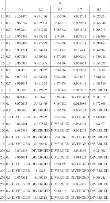
We chose L∗ _{= 1, which induces parallel anchoring and is typically more demanding} numerically than homeotropic anchoring. Results are collected in tables I-III. Tables I and II show, for two ρ∗

bulk values, the grand canonical potential, Ω, obtained for the full set of

h, η and α considered. In table III, summary data are presented showing the 1000- and 2000-epoch Ω values from batches of 10 equivalent runs withh= 10 and a range of ηand α

values. From these we conclude that:

1. The probability of divergence increases with h, η, α and ρ∗

bulk. We also observe that for smallh (less than 25) learning is fairly robust - there are no instances of repeated divergence, although in batches of 10 simulations, see table III, there were occasional simulations that diverged forη = 1.0,α = 0.9.

2. learning speed increases with η and α (as expected). Provided that h ≤ 25 we may, if convergence speed is important and occasional divergence can be accommodated, set η = 1.0 and α = 0.9. If, alternatively, divergence must be avoided, we should set

η= 0.7 and α= 0.9.

(17)

two, but the reduced computation time per epoch (and, hence, shorter overall time) could be an argument for choosing h= 10. That said, it is known that using a larger number of units leads to higher representation power. We therefore decided to select

h= 25 in our subsequent calculations using the MNN to determine the density profile to alternative boundary condition problems.

In summary, in what follows we employ (except where otherwise indicated) h= 25, η= 1.0 and α = 0.9. Convergence of the MNN was deemed to have been achieved if the difference (defined as in [11]) between two solutions 1000 iterations apart was less than 10−4_.

B. MNN vs iterative solution

We next assessed our new MNN method by comparing its results for the structure of a symmetric film with those obtained by standard iterative solution of the EL equation (8), and with computer simulations (NVT Monte Carlo forN = 1000 particles), where available Details of the simulations are given in [23, 24].

Once ρ(ω, z) has been found, we can integrate out the angular dependence to get the density profile,

ρ(z) = Z

ρ(z, ω)dω, (18)

and use this result to define the orientational distribution function (ODF) ˆf(z, ω) =

ρ(z, ω)/ρ(z), from which we can calculate the orientational order parameters in the laboratory-fixed frame [10]. These are the five independent components of the nematic order parameter tensor, Qαβ = h1₂(3ˆωαωˆβ −δαβ)i. In the case under study there is no twist, i.e., the director is confined to a plane that we can take as the xz plane and

Qyy =Qyz = 0. The three remaining order parameters, Qxy, Qzz and Qxz (because Qαβ is traceless, Qxx =−(Qxx+Qzz)), are in general all non-zero owing to surface-induced biaxi-ality, see our earlier work for L∗ _{= 1 [11]. This effect has not been neglected in the present} treatment, but in what follows we show results for Qzz only, as it (i) allows one readily to distinguish between homeotropic and planar states; and (ii) is usually the largest order parameter (in absolute value). It is given by

Qzz(z) = Z

(18)

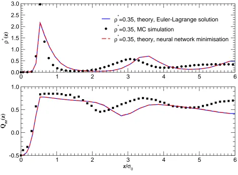
Figures 4–11 show the density and order parameter profiles from EL and MNN inimisation of the free energy, compared with MC simulation data. There is very good agreement between EL and MNN at the lower (isotropic) density, for all values of the reduced needle length L∗_{. At the higher (nematic) density, however, there is again perfect agreement for}

L∗ _{= 0, 1/3 and 1; for} _L∗ _{= 2}_/_{3, EL minimisation predicts alignment of the LC parallel to} the walls, as seen in simulations [23], whereas MNN with a single hidden layer predicts homeotropic alignment, which is metastable for this value of L∗_{. Indeed, we expect a} crossover from homeotropic to planar equilibrium alignment at L∗ _≈ ₀_._{5 [23], so it is not} altogether surprising that convergence to the absolute free energy minimum should be harder in this range, where bistability is often observed in simulations. Use of a MNN with two

hidden layers, however, allowed us to reach the correct equilibrium state at little extra computational cost, in three out of ten attempts, all starting from different random initial guesses for ρ(ω, z). In figure 9 we plot both the metastable and true equilibrium profiles, for which the free energy (in reduced units) is, respectively, 8.937 and 8.783. In the latter case there is again perfect agreement between the EL and MNN results. Note that the metastable state is also a solution of the EL equation, for a different choise of initial gueess.

C. Assessment of computational costs

In order to contrast the performances of MNN minimisation vs iterative solution of the EL equation, we ran three different codes on a laptop computer with a CPU of 2.20 GHz and 2 GB RAM, under the MS Windows Vista operating system. The confined HGO fluid parameters are κ = 3, L∗ _{= 1,} _ρ

bulk = 0.35, corresponding to the most demanding case of a bulk N phase between fully impenetrable walls. The EL code was run until the error, defined as the sum of the absolute values of the differences between consecutive iterates at 64×16×16 = 16384 points, was less than 10−2_{; the MNN was run for 1000 or 2000}

iterations.

A Standard iterative solution of the EL equation coded in C: runtime for 711 iterations is 436 minutes; final free energy is 8.965674.

(19)

as Matlab because Matlab uses machine code optimised for matrix calculation.

C MNN coded in Matlab, using h = 25 and pre-stored Kij matrix: runtime for 1000 iterations is 4 minutes. The Kij matrix, which is reusable for any simulation with the same model parameters, takes an additional 38 minutes to generate.

Storing the Kij matrix has obvious advantages in processing time, but we must remember that Kij is a huge matrix that uses 512 MB storage for this problem, making this approach very difficult to scale up to higher dimensions – the size of Kij increases quadratically with the number of Gaussian quadrature points included in any extra dimension.

Simulations of typesBandCare algorithmically equivalent, the only difference is whether or not matrix Kij is pre-stored, so the final free energies are the same. Results depend on the MNN parameterization, see table III; for η = 0.7, α = 0.9, the mean and median final free energy are, respectively, 8.959473 and 8.958575. This is within less than 0.1% of the EL result.

V. DISCUSSION AND CONCLUSIONS

We have developed and implemented a MNN for the grand-canonical functional of con-fined hard non-spherical particles. This has been tested for the HGO fluid treated at the level of the simple Onsager approximation with a ‘bulk’ Parsons-Lee scaling. Results were found to be in very good agreement with those from iterative solution of the EL equation, provided we use two hidden layers. Our MNN appears, however, to be substantially faster, which fact, coupled with its reliability, makes it a strong candidate for solving the structure of confined fluids. Speed and economy of memory storage are of particular importance if one wishes to consider systems where there is spatial variation in more than one dimension, or where the particles are biaxial, in which cases the EL-based method becomes at worst inapplicable, at best extremely expensive on computer resources. To see why this is so, con-sider a stripe-patterned substrate: now each particle needs to be specified by one additional spatial coordinate, say x, along the plane of the substrate. Hence the interaction kernel

Kij, equation (12), would depend on two additional variables, xi and xj; if we choose the number of integration points alongxto be, e.g.,nx = 32, thenKij would grow by a factor of

n2

(20)

coordinate is the third Euler angle, χ. By contrast, our MNN is sufficiently fast that Kij can be computed ‘on the fly’, with substantial RAM savings.

The MNN method as presented is general and can be applied to any functional of the density-orientation profile; we have tested it for the simplest possible, Onsager-like approxi-mation to the free energy of a fluid of hard rods. More sophisticated theoretical approaches are of course available, such as a weighted-density [42] or fundamental-measure [48, 49] ap-proximation, which would very likely be more accurate, i.e., reproduce simulations more closely, but our purpose, as stated above, was just to develop a new solution algorithm and assess its performance.

Our method can be fine-tuned in a number of ways, which might yield further perfor-mance/reliability gains. In particular more work needs to be done to ensure that we always converge to the true absolute minimum of the free energy, even when there are competing metastable states.

1. Symmetries. For systems with symmetric substrate conditions we may reduce the storage requirements by using an interaction matrix of size (nz/2)×nz (where nα is the number of discrete values of coordinate α); indeed, equivalent efficiencies can be achieved where there are any other planes of symmetry. Thus, if we assume that there are planes of symmetry perpendicular to the x, z and φ axes, the interaction matrix will scale as N = (n2

x/2)×(n2z/2)×n2θ ×(n2φ/2). Its size will then be N times the 8 bytes that are needed for representing high-precision floating-point numbers. For

nx =nz = 32, nθ =nφ= 16, this yields a total RAM requirement of 64 GB, which is achievable with high-end computational hardware and/or parallelisation.

2. Network topology. So far we have studied the impact on learning speed of varying the number of units within each layer, the learning rate and momentum factor, but not of increasing the number of hidden layers.

(21)

their weight update functions on the Hessian matrix, rather than the gradient of the energy. In a very large data set, finding the Hessian matrix is extremely time- and memory-consuming, which renders the Quasi-Newton approach unfeasible on a stan-dard computer. We have adapted the conjugate-gradient algorithm to compute the error gradient of the free energy for our unsupervised network (instead of the quadratic error of a standard MLP). We then used the Fletcher-Reeves update to compare the learning speed with that obtained with our backpropagation algorithm. This algo-rithm, like Pol´ak-Ribiere and Powell-Beale, requires a line-search to determine the minimum energy in a particular direction. This line-search is itself extremely time-consuming, and our experiments with Fletcher-Reeves have shown an overall learning speed slower than backpropagation. Moreover, convergence seemed more likely to become trapped in local minima. One possible solution would be to implement a scaled-conjugate-gradient algorithm [50]; these have been designed with the aim of avoiding the time consuming line-search of standard conjugate-gradient algorithms.

Given the above, the MLP approach would appear to offer a significant opportunity in the context of complex LC alignment calculations. There is no prospect of conventional iterative approaches being able to deal with cases with in-plane substrate variation, so this alternative is very welcome.

Acknowledgements

We thank D. de las Heras, L. Harnau, M. Schmidt and N. M. Silvestre for discussions.

This work was funded by the British Council under Treaty of Windsor grant no. B-54/07;

by the Portuguese Foundation for Science and Technology (FCT), through contracts no.

PTDC/FIS/098254/2008, Projecto Estrat´egico “Centro de F´ısica Te´orica e Computacional

2011-2011” PEst-OE/FIS/UI0618/2011, and EXCL/FIS-NAN/0083/2012; and by the UK

Engineering and Physical Research Council, Grant No. GR/S59833/01.

[1] http://www.displaybank.com/eng/.

(22)

[3] B. J´erˆome, Rep. Prog. Phys.54, 391 (1991). [4] T. J. Sluckin, Contemp. Phys.41, 37 (2000).

[5] G. P. Bryan-Brown, E. L. Wood and I. C. Sage, Nature 399, 338 (1999).

[6] C. V. Brown, M. J. Towler, V. C. Hui and G. P. Bryan-Brown, Liq. Cryst.27, 233 (2000). [7] N. A. Lockwood and N. L. Abbott, Current Opinion in Coll. Interf. Sci.10, 111 (2005). [8] P. Poulin, H. Stark, T. C. Lubensky and D. A. Weitz, Science 275, 1770 (1997).

[9] J. P. Hansen and I. R. McDonald,Theory of Simple Liquids, 2nd ed. (Academic Press, London, 1986).

[10] M. M. Telo da Gama, Molec. Phys.52, 611 (1984).

[11] A. Chrzanowska, P. I. C. Teixeira, H. Eherentraut and D. J. Cleaver, J. Phys.: Condens.

Matter13, 4715 (2001).

[12] D. de las Heras, L. Mederos and E. Velasco, Phys. Rev. E 68, 031709 (2003). [13] D. de las Heras, E. Velasco and L. Mederos, J. Chem. Phys.120, 4949 (2004).

[14] J. P. Bramble, S. D. Evans, J. R. Henderson, C. Anquetil, D. J. Cleaver and N. J. Smith, Liq.

Cryst. 34, 1059 (2007).

[15] Y. Yi, V. Khire, C. Bowman, J. Maclennan and N. Clark, J. Appl. Phys.103, 093518 (2008). [16] C. Anquetil-Deck and D. J. Cleaver, Phys. Rev. E 82, 031709 (2010).

[17] C. Anquetil-Deck, D. J. Cleaver and T. J. Atherton, Phys. Rev. E86, 041707 (2012). [18] S. Kitson and A. Giesow, App. Phys. Lett. 803635 (2002).

[19] C. Tsoktas, A. J. Davidson, C. V. Brown and N. J. Mottram, App. Phys. Lett. 90 111913 (2007).

[20] G. G. Wells and C. V. Brown, Appl. Phys. Lett.91, 223506 (2007).

[21] S. Haykin,Neural Networks: A Comprehensive Foundation, 2nd ed. (Prentice-Hall, 1998). [22] K. Hornik, M. Stinchcombe and H. White, Neural Networks 2, 359 (1989).

[23] P. I. C. Teixeira, F. Barmes and D. J. Cleaver, J. Phys.: Condens. Matter 16, S1969 (2004). [24] P. I. C. Teixeira, F. Barmes, C. Anquetil-Deck and D. J. Cleaver, Phys. Rev. E 79, 011709

(2009).

[25] H. Bourlard, N. Morgan and S. Renals, Speech Comm.11, 237 (1992).

[26] J. Guti´errez and Ali S. Hadi, Expert Systems and Probabilistic Network Models (Springer-Verlag, Berlin, 1997).

(23)

[28] F. Rosenblatt, Principles of Neurodynamics: Perceptrons and the Theory of Brain Mechanisms

(Spartan, Washington DC, 1962).

[29] N. Intrator, Neural Computation4, 98 (1992).

[30] M. Gardner and S. Dorling, Atmospheric Environment34, 21 (2000). [31] C. M. Care and D. J. Cleaver, Rep. Prog. Phys. 68, 2665 (2005). [32] M. Rigby, Molec. Phys.68, 687 (1989).

[33] J. W. Perram and M. S. Wertheim, J. Comput. Phys. 58, 409 (1985); J. W. Perram, J. Rasmussen, E. Praestgaard and J. L. Lebowitz, Phys. Rev. E 54, 6565 (1996).

[34] M. P. Allen, G. T. Evans, D. Frenkel and B. M. Mulder, Adv. Chem. Phys. 86, 1 (1993). [35] V. R. Bhethanabotla and W. Steele, Molec. Phys.60, 249 (1987).

[36] S. L. Huang and V. R. Bhethanabotla, Int. J. Mod. Phys. C10, 361 (1999). [37] E. Velasco and L. Mederos, J. Chem. Phys. 109, 2361 (1998).

[38] D. J. Cleaver and P. I. C. Teixeira, Chem. Phys. Lett. 338, 1 (2001). [39] R. Evans, Adv. Phys. 28, 143 (1979).

[40] A. Poniewierski, Phys. Rev. E 47, 3396 (1993).

[41] J. D. Parsons, Phys. Rev. A19,1225 (1979); S. D. Lee, J. Chem. Phys. 78, 4972 (1987). [42] A. M. Somoza and P. Tarazona, J. Chem. Phys. 91, 517 (1989); E. Velasco, L. Mederos and

D. E. Sullivan, Phys. Rev. E 62, 3708 (2000). [43] A. Chrzanowska, J. Comput. Phys. 191, 265 (2003).

[44] W. McCulloch and W. Pitts, Bull. Math. Biophys. 7, 115 (1943).

[45] See, e.g., W. H. Press, S. A. Teukolsky, W. T. Vetterling, B. P. Flannery, Numerical Recipes

in C : The Art of Scientific Computing, second ed. (Cambridge University Press, Cambridge,

1993).

[46] D. F. Specht, Neural Networks 3, 109 (1990).

[47] D. S. Modha and Y. Fainman, IEEE Trans. Neural Networks5, No. 3 (1994). [48] H. Hansen-Goos and K. Mecke, Phys. Rev. Lett.102, 018302 (2009).

[49] R. Wittmann and K. Mecke, J. Chem. Phys. 140, 104703 (2014).

(24)

α

h η 0.1 0.3 0.5 0.7 0.9

10 0.1 1.18672 1.144328 1.137906 1.138144 1.155396

10 0.4 1.143171 1.137942 1.138922 1.148959 1.138407

10 0.7 1.137403 1.135984 1.146504 1.139451 1.135816

10 1.0 1.136813 1.138326 1.135614 1.135183 1.134833

25 0.1 1.155936 1.146062 1.139696 1.137812 1.151736

25 0.4 1.142638 1.138965 1.137261 1.149138 1.140928

25 0.7 1.137169 1.136048 1.147395 1.137414 1.136469

25 1.0 1.135599 1.139655 1.135423 1.134769 1.134763

50 0.1 1.161899 1.147519 1.139771 1.138908 1.150827

50 0.4 1.143001 1.1393 1.137638 1.14981 1.145919

50 0.7 1.13813 1.136625 1.14542 1.138345 1.136331

50 1.0 1.135791 1.139874 1.13528 1.135041 1.134815

100 0.1 1.153975 1.143765 1.141101 1.138393 1.150638

100 0.4 1.142178 1.139652 1.137911 1.149062 1.141389

100 0.7 1.138173 1.136224 1.146931 1.138316 1.135955

100 1.0 1.135891 1.13979 1.135491 1.16345 1.134821

150 0.1 1.151959 1.143478 1.141839 1.139804 1.148809

150 0.4 1.141686 1.140083 1.138062 1.147389 1.139929

150 0.7 1.138489 DIVERGED 1.144011 1.138239 1.136154

150 1.0 DIVERGED 1.139816 1.135752 1.135015 1.135209

200 0.1 1.150801 1.143571 DIVERGED 1.137666 1.149625

200 0.4 1.141804 1.139046 1.13702 1.147081 1.140075

200 0.7 DIVERGED DIVERGED 1.144176 1.138129 DIVERGED

200 1.0 DIVERGED 1.139729 1.135639 DIVERGED 1.135132

250 0.1 1.153768 1.142571 1.140022 DIVERGED 1.148498

250 0.4 1.140632 DIVERGED DIVERGED 1.147263 DIVERGED

250 0.7 DIVERGED DIVERGED 1.143332 DIVERGED DIVERGED

[image:24.595.128.487.73.735.2]

250 1.0 DIVERGED 1.138431 1.13553 DIVERGED DIVERGED

(25)

α

h η 0.1 0.3 0.5 0.7 0.9

10 0.1 9.101475 8.971296 8.955008 8.963734 9.023824

10 0.4 8.966737 8.962024 8.962016 8.999954 8.955046

10 0.7 8.952314 8.954215 8.966831 8.951803 8.968915

10 1.0 8.959308 8.965214 8.94864 8.967841 8.948766

25 0.1 9.032404 8.977229 8.954232 8.965194 9.030154

25 0.4 8.974211 8.953414 8.971946 8.99511 8.962507

25 0.7 8.970363 8.959918 8.979666 8.950231 8.959656

25 1.0 8.950319 8.961905 8.957792 8.958059 8.957027

50 0.1 9.09479 8.959672 8.964864 8.962899 9.015685

50 0.4 8.976157 8.953012 8.952501 8.99655 8.96172

50 0.7 8.961037 8.961134 8.973959 8.969405 8.958759

50 1.0 8.949888 8.972432 8.958441 8.947867 DIVERGED

100 0.1 9.091432 8.97678 8.96335 DIVERGED 9.031278

100 0.4 8.972937 8.962469 8.966482 9.013989 8.972309

100 0.7 8.969883 DIVERGED 8.985739 8.960194 DIVERGED

100 1.0 DIVERGED 8.952872 8.948058 DIVERGED 9.149149

150 0.1 9.065501 8.957815 DIVERGED 8.963453 9.03997

150 1.0 DIVERGED 8.962265 DIVERGED DIVERGED DIVERGED

200 0.1 9.077518 DIVERGED DIVERGED 8.963536 9.034062

200 1.0 DIVERGED 8.9528 DIVERGED DIVERGED DIVERGED

250 0.1 9.057811 8.990148 DIVERGED DIVERGED 9.008942

250 0.4 DIVERGED DIVERGED DIVERGED 8.995841 DIVERGED

[image:25.595.128.487.75.733.2]

(26)

η= 1.0,α= 0.9 η= 1.0,α= 0.7 η = 0.7,α= 0.9 η= 0.7,α= 0.7

1000 2000 1000 2000 1000 2000 1000 2000

Mean 8.964565* 8.957609* 8.968601 8.965057 8.961541 8.959473 8.970223 8.962241

Median 8.960294 8.958088 8.969784 8.965568 8.960423 8.958575 8.970974 8.962251

Maximum DIVERGED DIVRGED 8.975090 8.971631 8.970380 8.968318 8.977538 8.972639

Minimum 8.949732 8.948179 8.955962 8.952717 8.951463 8.949201 8.957841 8.951727

[image:26.595.75.533.72.224.2]

St. deviation 0.016548* 0.008898* 0.006345 0.006298 0.006714 0.006718 0.006962 0.006562

TABLE III: Grand canonical potential Ω values after 1000 and 2000 MNN epochs, forh= 10 and

different choices of momentum and learning step parameters. The HGO model parameters are

κ= 3, ρ∗

bulk = 0.35 (bulk N phase) andL∗ = 1 (impenetrable walls). Statistics are compiled from

(27)

(a)

(b)

FIG. 1: (a) A neurone fires (or not) on the basis of the stimuli it receives from other neurones. (b)

[image:27.595.83.531.70.694.2]

(28)

[image:28.595.176.423.75.255.2]

FIG. 2: Example of MLP with 3 units in the input layer, 5 units in the hidden (intermediate) layer

and 2 units in the output layer.

σ

0

σ

z

L

wall

θ

L

FIG. 3: The HNW potential: the molecules see each other (approximately) as uniaxial hard

ellipsoids of axes (σ0, σ0, κσ0), but the wall sees a molecule as a hard line of lengthL, which need

not equal κσ0. Physically, this means that molecules are able to embed their side groups into the

bounding walls. VaryingLis therefore equivalent to changing the wall penetrability, which can be

[image:28.595.163.448.376.583.2]

(29)

0 1 2 3 4 5 6

z/σ₀

-0.5 0.0 0.5 1.0

Q zz

(z)

0 1 2 3 4 5 6

0.0 0.5 1.0 1.5 2.0

ρ

∗ (z)

ρ*

=0.28, theory, Euler-Lagrange solution

ρ*

=0.28, MC simulation

ρ*

[image:29.595.73.540.73.414.2]

=0.28, theory, neural network minimisation

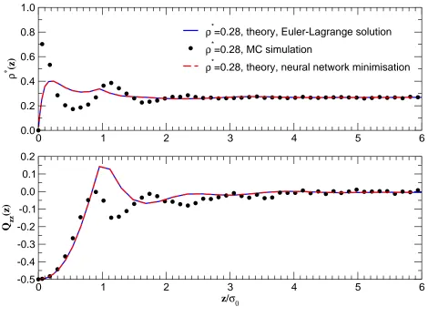
FIG. 4: Density ρ∗(z) (top) and order parameter Qzz(z) (bottom) profiles for a symmetric film

of HGO particles of elongation κ = 3, for ρ∗_bulk = 0.28. The needle length is L∗ = 0 on both walls, inducing homeotropic anchoring (only one half of system is shown). Lines are from theory

using the standard solution of the EL equation (solid) and our MNN (dashed), symbols are from

(30)

0 1 2 3 4 5 6

z/σ₀

-0.5 0.0 0.5 1.0

Q zz

(z)

0 1 2 3 4 5 6

0.0 0.5 1.0 1.5 2.0

ρ

∗ (z)

ρ*

[image:30.595.75.541.72.413.2]

(31)

0 1 2 3 4 5 6

z/σ₀

-0.5 0.0 0.5 1.0

Q zz

(z)

0 1 2 3 4 5 6

0.0 0.5 1.0 1.5

ρ

∗ (z)

ρ*

[image:31.595.71.541.73.417.2]

of HGO particles of elongation κ = 3, for ρ∗_bulk = 0.28. The needle length is L∗ = 1/3 on both walls, inducing homeotropic anchoring (only one half of system is shown). Lines are from theory

using the standard solution of the EL equation (solid) and our MNN (dashed), symbols are from

(32)

0 1 2 3 4 5 6

z/σ₀

-0.5 0.0 0.5 1.0

Q zz

(z)

0 1 2 3 4 5 6

0.0 0.5 1.0 1.5 2.0 2.5 3.0

ρ

∗ (z)

ρ*

[image:32.595.72.540.70.414.2]

(33)

0 1 2 3 4 5 6

z/σ₀

-0.5 -0.4 -0.3 -0.2 -0.1

0.0 0.1 0.2

Q zz

(z)

0 1 2 3 4 5 6

0.0 0.2 0.4 0.6 0.8 1.0

ρ

∗ (z)

ρ*

[image:33.595.71.541.69.417.2]

FIG. 8: Densityρ∗(z) (top) and order parameter Qzz(z) (bottom) profiles for a symmetric film of

HGO particles of elongation κ= 3, for ρ∗_bulk = 0.28. The needle length is L∗ = 2/3 on both walls, inducing parallel anchoring (only one half of system is shown). Lines are from theory using the

standard solution of the EL equation (solid) and our MNN (dashed), symbols are from simulation.

(34)

0 1 2 3 4 5 6

z/σ₀

-0.5 0.0 0.5 1.0

Q zz

(z)

0 1 2 3 4 5 6

0.0 0.5 1.0 1.5

ρ

∗ (z)

ρ*

=0.35, theory, neural network minimisation (metastable)

ρ*

[image:34.595.72.541.71.434.2]

=0.35, theory, neural network minimisation (stable)

FIG. 9: Same as figure 8, but forρ∗

bulk = 0.35. This density lies in the nematic phase. MNN results

were calculated using two two hidden layers, η = 1.0 and α = 0.97. The meatastable profiles are

(35)

0 1 2 3 4 5 6

z/σ₀

-0.5 -0.4 -0.3 -0.2 -0.1

0.0

Q zz

(z)

0 1 2 3 4 5 6

0.0 0.2 0.4 0.6 0.8 1.0

ρ

∗ (z)

ρ*

[image:35.595.72.540.70.415.2]

of HGO particles of elongationκ= 3, forρ∗_bulk = 0.28. The needle length isL∗ = 1 on both walls, inducing parallel anchoring (only one half of system is shown). Lines are from theory using the

standard solution of the EL equation (solid) and our MNN (dashed), symbols are from simulation.

(36)

0 1 2 3 4 5 6

z/σ₀

-0.5 -0.4 -0.3 -0.2 -0.1

0.0

Q zz

(z)

0 1 2 3 4 5 6

0.0 0.5 1.0 1.5 2.0

ρ

∗ (z)