The polyhedral Gauss map and discrete curvature
measures in geometric modelling.
ECHEVERRIA, Gilberto.
Available from Sheffield Hallam University Research Archive (SHURA) at:
http://shura.shu.ac.uk/19598/
This document is the author deposited version. You are advised to consult the
publisher's version if you wish to cite from it.
Published version
ECHEVERRIA, Gilberto. (2007). The polyhedral Gauss map and discrete curvature
measures in geometric modelling. Doctoral, Sheffield Hallam University (United
Kingdom)..
Copyright and re-use policy
Adsetfs Centre City Campus Sheffield SI 1WB 1 0 1 859 8 87 1
Return
to
Learning Centre of issue
Fines are charged
at
50p per
hour
ProQuest Number: 10694479
All rights reserved INFORMATION TO ALL USERS
The quality of this reproduction is dependent upon the quality of the copy submitted. In the unlikely event that the author did not send a com plete manuscript and there are missing pages, these will be noted. Also, if material had to be removed,
a note will indicate the deletion.
uest
ProQuest 10694479
Published by ProQuest LLC(2017). Copyright of the Dissertation is held by the Author.
All rights reserved.
This work is protected against unauthorized copying under Title 17, United States C ode Microform Edition © ProQuest LLC.
ProQuest LLC.
789 East Eisenhower Parkway P.O. Box 1346
The Polyhedral Gauss Map and discrete curvature measures in
geometric modelling
Gilberto Echeverria
A thesis submitted in partial fulfilment of the requirements of Sheffield Hallam University
for the degree of Doctor of Philosophy
Sheffield Hallam University Materials & Engineering Research Institute
The undersigned hereby certify that they have read and recommend to the Faculty of Arts, Computing, Engineering and Sciences for acceptance a thesis entitled “The Polyhedral Gauss M ap and discrete curvature measures in geometric modelling” by Gilberto Echeverria in partial fulfillment of the requirements for the degree of Doctor of Philosophy.
Dated: 05 July 2007
Research Supervisors: _______________________________ Professor Marcos Rodrigues
Dr Lyuba Alboul
Examining Committee: _______________________________________ Professor Ruud Van Damme (University of Twente)
Sheffield Hallam University
Date: 05 July 2007
Author: Gilberto Echeverria
Title: The Polyhedral Gauss M ap and discrete curvature measures in geometric modelling
Department: M aterials & Engineering Research Institute Degree: Ph.D. Convocation: 05 July 2007 Year:
Permission is herewith granted to Sheffield Hallam University to circulate and to have copied for non-commercial purposes, at its discretion, the above title upon the request of individuals or institutions.
THE AUTHOR ATTESTS THAT PERMISSION HAS BEEN OBTAINED FOR THE USE OF ANY COPYRIGHTED MATERIAL APPEARING IN THIS THESIS (OTHER THAN BRIEF EXCERPTS REQUIRING ONLY PROPER ACKNOWLEDGEMENT IN SCHOLARLY WRITING) AND THAT ALL SUCH USE IS CLEARLY ACKNOWLEDGED.
Signature of Author
Contents
List of Tables
ix
List of Figures
x
List of Algorithms
xvi
Abstract
* xvii
Acknowledgements
xviii
List of Publications
xix
1 Introduction and problem statement
1
1.1 Aims of the research p r o je c t... 4
1.2 Experimental m ethodology... 6
1.3 Main research contributions ... 8
1.4 Organisation of the th e sis ... 9
2 Geometric concepts and discrete curvature in two dimensions
11
2.1 Introduction... 112.2 Basic geometric concepts and computational im plem entations... 12
2.3 Notions related to the concept of curvature... 20
2.3.1 Formulae and definitions... 20
2.3.2 Spherical image of a curve and curvature identical curves 29
2.4 Potential applications of T A C ... 30
2.4.1 Curve reconstruction from point c lo u d s ... 31
2.4.2 Face recognition by curvature of face p ro files... 35
2.5 C onclusions... 37
3 Discrete curvature in three dimensions
38
3.1 Introduction... 38
3.1.1 Previous research on Gauss M a p s ... 40
3.1.2 Existing applications using Gauss M a p s ... 41
3.2 Basic concepts and d efin itio n s... 43
3.2.1 Polyhedral s u r f a c e ... 43
3.2.2 Integral Gaussian curvature and the angle d e f ic it... 44
3.2.3 Integral absolute curvature and its discrete analogue ... 45
3.3 The Polyhedral Gauss M a p ... 50
3.4 Analysis of the validity of the Polyhedral Gauss M a p ... 52
3.5 C onclusions... 62
4 Computational implementation of the Polyhedral Gauss Map
64
4.1 Introduction... 644.2 Overview of the g au ssM ap p ro g ra m ... 65
4.2.1 Data in p u t... 66
4.2.2 Program o u tp u t... 67
4.2.3 Algorithm to compute the Polyhedral Gauss M a p ... 68
4.3 Step-by-step explanation of the algorithm ... 71
4.3.1 Face ordering around v ... 71
4.3.2 Normal star and spherical in d icatrix ... 71
4.3.3 Detection of arc intersections... 72
4.3.4 Matching of intersection v ecto rs... 76
4.3.5 Splitting into spherical polygons... 79
4.3.6 Area of the spherical polygons... 81
4.3.7 Determining the orientation of a spherical p o ly g o n ... 82
4.3.8 Special c a s e s ... 85
4.3.9 Computational complexity of the alg o rith m ... 86
4.4 Examples of curvature measures using P G M ... 87
4.5 Results and potential applications ...1 ... 91
4.5.1 Comparison of the Angle Deficit and the Polyhedral Gauss Map . 91 4.5.2 Object recognition based on curvature... 94
4.5.3 Terrain description and navigation... 95
4.5.4 Polyhedral mesh subdivision or simplification... 97
4.6 Conclusions . ... 99
5 Visual display of the Polyhedral Gauss Map with 3D graphics
101
5.1 Introduction... 101
5.2 Other visualisations of the Gauss M a p ... 102
5.3 Display of the PGM with O p en G L ...103
5.3.1 Visualisation of the spherical in d ic a trix ... 103
5.3.2 The ro ta te T o X Y p la n e fu n c tio n ...106
5.3.3 Spherical polygons with O p e n G L ... 107
5.3.4 Triangulation of spherical p o ly g o n s...108
5.4 Interaction with the d isp lay ... 110
5.5 Solving problems of the Gauss Map using the visualisation... 113
5.6 C onclusions...114
5.7 Future research directions... 114
6 Triangle mesh simplification using the Polyhedral Gauss Map
116
6.1 Introduction...1166.2 Previous research on mesh simplification... 118
6.3 Curvature as decimation param eter... 121
6.3.1 TAC w eig h t...122
6.3.2 ATAC w e ig h t... 122
6.3.3 PTAC w e ig h t... 122
6.3.4 LTAC w e ig h t... 123
6.4 Implementation of a vertex decimation a lg o rith m ...125
6.4.1 Optimisation of the triangulation using edge f lip s ...127
6.5 Experimental results ... 129
6.6 Potential applications of a curvature guided simplification...133
6.7 Conclusions...134
6.8 Future research directions...136
7 Conclusions and further research
137
7.1 Conclusions...1377.2 Future research directions...139
Bibliography
140
A Curve-fitting over datasets on a plane
148
A .l Introduction... . 148A.2 Previous research on curve reconstruction... 150
A.3 Details of the implementation... 152
A.3.1 Data in p u t...152
A.3.2 Program o u tp u t... 153
A.4 Simple closed curves by o rie n ta tio n ... 154
A.4.1 Self-intersections... 157
A.5 Curves with one deviation from the convex h u l l ...160
A.5.1 By distances ... 162
A.5.2 By a n g le s...165
A.5.3 Self-intersections...167
A.6 Curves with multiple deviations ... 170
A.6.1 Self-intersections ... 183
A.7 Results and evaluation of the algorithm s...184
List of Tables
List of Figures
1.1 Example of curve-fitting using the r e c o n s t r u c t o r program... 7
1.2 Example of Polyhedral Gauss Map of a vertex from the g au ssM ap pro gram 7 1.3 Example of polygon simplification with the d e c im a to r program. . . . 8
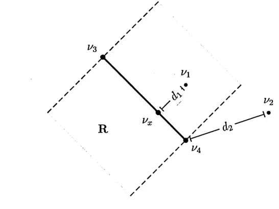
2.1 Distance from a point to a segment. Sweep region R shown in grey. . . . 15
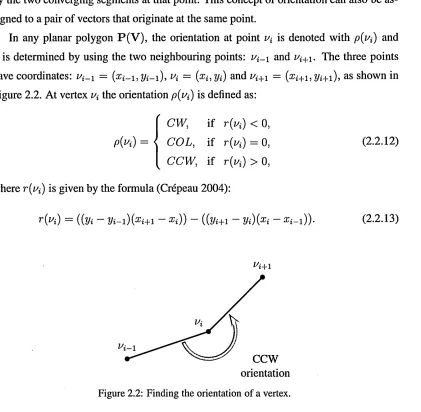
2.2 Finding the orientation of a vertex... 16
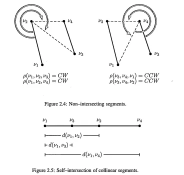
2.3 Determining self-intersections based on orientation... 18
2.4 Non-intersecting segments... 18
2.5 Self-intersection of collinear segments... 18
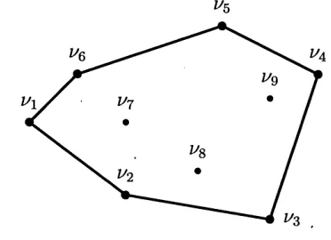
2.6 Convex hull of a point cloud ... 19
2.7 Selection of vertices belonging to the convex hull of a dataset, based on orientation... 20
2.8 A curve with discontinuity points si and s2... 21
2.9 The TAC of a convex curve is always equal to 27r. . ... 22
2.10 General case with several convex and concave angles... 23
2.11 Deviation angles in a non-convex curve. The deviating angle at vertex vA is formed by the deviating segment and the (imaginary) segment Fpq belonging to the CH-curve. At vertex V\ the deviation angle is formed by segments Fpq and FjTTio... 24
2.12 Relationship between internal and external angles in a triangle... 26
2.13 Sum of angles of a polygon with one deviation and no internal convex vertices... 26
2.14 Changes in the angles of a polygon due to the insertion of a new vertex. . 27
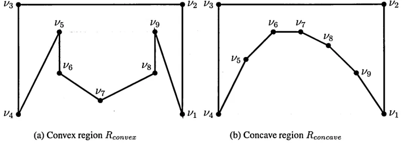
2.15 Convex and concave regions, shown in g re y ... 27
2.16 Insertion of a vertex into a convex region... 28
2.19 Nested convex hulls of a dataset... 31
2.20 A bridge delimited by two link segments, in a dataset with two layers. . . 32
2.21 Curve with minimum amount of link segments. In the data k = 3, and there are 3 link segments... 32
2.22 Curve with maximum amount of link segments. In the data k = 3, and there are 4 link segments... 33
2.23 Concentric circles with vertices aligned... 34
2.24 Original source of the data: curve P (V )sau;... 34
2.25 Concentric circles with inner circle rotated... 35
2.26 Rotated concentric circles with smaller 5r... 35
2.27 Example profiles used for face recognition by curvature measures... 37
3.1 Gauss Map of a smooth surface... 44
3.2 Computation of the Gaussian curvature (a;) around vertex v... 45
3.3 Two polyhedra with similar Gaussian curvatures... 46
3.4 Vertex types identified using the Total Absolute Curvature... 47
3.5 Mixed vertex where all faces have at least one deviation edge... 48
3.6 Mixed vertex where some faces do not have any deviation edges... 50
3.7 Construction of the spherical indicatrix of a convex vertex... 51
3.8 Two kinds of vertices with their spherical indicatrices... 52
3.9 Ordering of the faces and corresponding normal vectors around a vertex. . 53
3.10 PGM of the basic types of vertices... 54
3.11 Projection of a neighbour vertex on a plane... 54
3.12 Mixed vertex and top-down view showing the faces and vertices... 57
3.13 Convex cone representing the negative part of the curvature of a mixed vertex... 57
3.14 Self-intersecting mixed vertex and top-down view showing the vertices. . 59
3.15 Mixed vertex with self-intersection... 59
3.16 A ‘figure-8’ vertex... 60
3.17 A ‘pinch’ vertex... 60
3.18 Extension of the faces in a saddle vertex to create its dual convex cone. . . 61
4.1 Simple vertices and their spherical indicatrices... 68
4.2 A vertex with positive and negative areas in its Gauss Map... 68
4.3 Special case of three vectors forming a line in the spherical indicatrix. . . 72
4.4 Gauss map of a vertex with two coplanar faces... 73
4.5 Intersection of two arcs defined by the normal vectors at their endpoints. . 73
4.6 Intersection of two arcs. The planes defined by the arcs are shown. The vectors, the arc and the plane use the same colour. The intersection line is shown in red... 74
4.7 The e n d p o in t variable as a four bit number, representing the four vec tors involved in an arc intersection 74
4.8 Arcs that do not intersect. In this case the intersection line is outside of at least one of the arcs... 75
4.9 Planar representation of the spherical indicatrix, showing the intersection vectors... 76
4.10 Different cases of arc intersections... 77
4.11 Gauss Map of a cone with several intersections on the spherical indicatrix and overlapping spherical polygons... 79
4.12 Planar representation of the spherical indicatrix, showing the intersection vectors... 80
4.13 Indicatrix after the removal of the first spherical polygon... 80
4.14 Indicatrix after the removal of the second spherical polygon. There are no more intersections, thus the indicatrix represents now the last spherical polygon... 81
4.15 Gauss Map of a vertex with a self-intersection... 83
4.16 Vertices with overlapping and cancelling spherical polygons... 84
4.17 PGM of a vertex, showing the normal of the vertex in magenta colour. . . 85
4.18 A complex mixed vertex and its spherical indicatrix (left) and PGM (right). 88 4.19 PGM of the monkey saddle... 88
4.20 PGM of a generalised monkey saddle... 89
4.21 PGM of the tulip vertex... 89
4.22 Pinch vertex with the corresponding Gauss Map... 90
4.23 Reverse pinch vertex with the corresponding Gauss Map... 90
4.24 Cone-eight vertices of increasing height... 91
4.25 Vertex classification of the two polyhedra. Left: Angle Deficit classifica tion. Right: Polyhedral Gauss Map classification... 93
4.26 Visualisations of the initial torus, coloured by curvature, highlighting the curvature of a selected vertex... 94
4.28 Another optimised torus, coloured by curvature, highlighting the curva
ture of a selected vertex... 95
4.29 AD and PGM visualisations of a simplified venus model... 95
4.30 AD and PGM visualisations of a triceratops model... 95
4.31 Various meshes with vertices colour coded according to their characteri sation using the two methods. Measures of curvature using Angle Deficit (centre) and Polyhedral Gauss Map (Right)... 96
4.32 Use of curvature for terrain navigation. Top: Terrain meshes. Middle: Direct path. Bottom: Path based on curvature... 98
4.33 Subdivision of a mixed vertex to generate two vertices, one positive and one negative... 99
5.1 Visualisation of the normal star of a vertex...104
5.2 Initial visualisation of the spherical indicatrix...105
5.3 Initial visualisation of the areas of the Polyhedral Gauss Map... 105
5.4 The parameters for the gluPartialDisk function... 106
5.5 Using arcs to join the normal vectors...107
5.6 Truncated saddle vertex. Its PGM has a non-convex spherical polygon. . 109
5.7 Two cases of ear-slicing for polygon triangulation... 110
5.8 A triangle on a sphere, drawn using 3 clipping planes to segment a red sphere... 110
5.9 Showing the ID numbers of faces and vectors. Intersection vectors have negative ID numbers... I l l 5.10 Toggling of the display of spherical polygons according to their sign. . . . 112
5.11 Display of the projected link of a vertex...112
5.12 Separation of the spherical polygons by scaling them by a small factor. . . 115
6.1 Triceratops model: shaded (left), wireframe (right)... 117
6.2 Comparison of the vertex weight parameters: TAC, ATAC, PTAC and LTAC. 124 6.3 Triceratops model simplified with LTAC to 84.4%...125
6.4 Edge flip and inverse edge flip of an edge... 128
6.5 Comparison of the triangulations obtained after removal of a saddle ver tex... 129
6.6 Venus model: shaded (left), wireframe (centre), curvature coded (right). . 130.
6.8 Rockerarm model: shaded (left), wireframe (right)... 133
6.9 Detail of the decimated rockerarm model at 95 % decimation...134
6.10 Skeletalfoot model: shaded (left), wireframe (right)... 135
6.11 Textured triceratops at three levels of detail. Mesh simplified, from front to back, at 0,70.6 and 88.3 % decimation, respectively. ... 135
A. 1 The four datasets used for the curve reconstruction algorithms. 155 A.2 Generation of a simple closed curve based on orientation...155
A.3 Special case of vertices collinear with vr... 158
A.4 Self-intersection caused by collinear points at the end of the dataset. . . . 158
A.5 Self-intersection caused by collinear points at the right of the dataset. . . 159
A.6 Self-intersections in the curve created...159
A.7 Curves obtained using the orientation algorithm... . 160
A. 8 Nested convex hulls of a dataset... 161
A.9 The four test datasets showing the layers with different colours... 161
A. 10 Breaking the hulls at blank segments and joining them with link segments. 162 A. 11 Dataset with two layers of nested convex hulls... 163
A. 12 Convex hull layers linked to form a single curve... 164
A. 13 Curves with one deviation. The layers are joined using one distance. . . . 164
A. 14 Curves with one deviation. The layers are joined using two distances. . . 165
A. 15 Curve not found by the algorithm...165
A. 16 Joining hulls by angles, the curve with the smallest curvature is chosen. . 166
A. 17 Self-intersection when joining two hulls...166
A. 18 Curves with one deviation. The layers are joined using two distances. . . 167
A. 19 Intersection of the link segments joining two layers... 167
A.20 Intersection of the inner convex hull with a new link segment...168
A.21 Test triangle to identify self-intersections...168
A.22 Intersection of an intermediate convex hull...169
A.23 Intersection of an intermediate hull at one of the vertices...170
A.24 Adding vertices to the convex hull to fit a curve over the whole dataset. Point cloud (a), convex hull (b), points added in sequence (c-e) and final curve (f)...172
A.25 Measurements used as minimisation parameters for the selection of vertices. 173 A.26 Curves with multiple deviations using / (z/e) = u... 174
A.27 Curves with multiple deviations using /( ^ e) = de... 174
A.29 Curves with multiple deviations using /( ^ e) A.30 Curves with multiple deviations using /( ^ e) A.31 Curves with multiple deviations using f (v e) A.32 Curves with multiple deviations using /( ^ e) A.33 Curves with multiple deviations using f ( v e) A.34 Curves with multiple deviations using / ( ^ e) A.35 Curves with multiple deviations using /(^e) A.36 Curves with multiple deviations using /( ^ e) A.37 Curves with multiple deviations using f { v e) A.38 Curves with multiple deviations using f{ ve) A.39 Curves with multiple deviations using f ( v e) A.40 Curves with multiple deviations using f ( v e) A.41 Curves with multiple deviations using /(i/e) A.42 Curves with multiple deviations using /(V e) A.43 Curves with multiple deviations using / ( ^ e) A.44 Curves with multiple deviations using f ( v e) A.45 Curves with multiple deviations using f { v e) A.46 Curves with multiple deviations using f ( v e) A.47 Curves with multiple deviations using f ( v e) A.48 Curves with multiple deviations using /( ^ e)
de 175
I1+/2... f ...17645 a i...176 a i + a 2 + a 3... 176
0 ^ 1 + y ... 177 &i(h + l2) for three angles. 177 a ^ h h )...178 ai(l\l2) for three angles. . 178
f i s ... 178 for three angles. . . . 179
-av...179
for three angles. . . 180
(h)
...180
^ ( ^ ) for three angles. 180 a l + a% + a | ... 181 ( ^ ) for three angles. . 181 t5 x ) for three angles. 182 ' l + '2 /a\ for three angles. 182 (al(lil2)) for three angles. 182 • • 183
List of Algorithms
4.1 Polyhedral Gauss Map... 70
A .l Curve-fitting based on orientation...156
A.2 Curve-fitting with one deviation...163
Abstract
The Work in this thesis is concentrated on the study of discrete curvature as an important geometric property of objects, useful in describing their shape. The main focus is on the study of the methods to measure the discrete curvature on polyhedral surfaces. The curva tures associated with a polyhedral surface are concentrated around its vertices and along its edges. An existing method to evaluate the curvature at a vertex is the Angle Deficit, which also characterises vertices into flat, convex or saddle. In discrete surfaces other kinds of vertices are possible which this method cannot identify. The concept of Total Absolute Curvature (TAC) has been established to overcome this limitation, as a mea sure of curvature independent of the orientation of local geometry. However no correct implementation of the TAC exists for polyhedral surfaces, besides very simple cases.
For two-dimensional discrete surfaces in space, represented as polygonal meshes, the TAC is measured by means of the Polyhedral Gauss Map (PGM) of vertices. This is a rep resentation of the curvature of a vertex as an area on the surface of a sphere. Positive and negative components of the curvature of a vertex are distinguished as spherical polygons on the PGM. Core contributions of this thesis are the methods to identify these polygons and give a sign to them. The PGM provides a correct characterisation of vertices of any type, from basic convex and saddle types to complex mixed vertices, which have both positive and negative curvature in them.
Another contribution is a visualisation program developed to show the PGM using 3D computer graphics. This program helps in the understanding and analysis of the results provided by the numerical computations of curvature. It also provides interactive tools to show the detailed information about the curvature of vertices.
Acknowledgements
I would like to thank my supervisor, Dr. Lyuba Alboul, for her patience and guidance in a field of knowledge which was new to me. I would also like to give thanks to my director of studies, Professor Marcos Rodrigues, for providing me with the opportunity to undertake this research program. Also would like to acknowledge all other members of the research team: Jacques Penders, Georgios Chliveros, Alan Robinson and Willie Brink, who shared their time and knowledge with me, and provided useful advice.
List of Publications
• Echeverria, G. and L. Alboul (2007). Shape-preserving mesh simplification based on curvature measures from the Polyhedral Gauss Map. International Journal on Computational Vision and Biomechanics. Received: 26/02/2007. Accepted:
17/05/2007.
• Echeverria, G. and L. Alboul (2006, October 20-21). Decimation and smoothing of triangular meshes based on curvature from the polyhedral gauss map. In Proc. O f CompIMAGE Conference. Coimbra, Portugal, pp. 175-180.
• Echeverria, G., L. Alboul, and M. Rodrigues (2005, November 24-25). Enhancing game physics using gauss map computation. In Proc. O f Game-On Conference. Leicester, UK, pp. 47-51.
• Alboul, L. and G. Echeverria (2005, September 5-7). Polyhedral Gauss maps and curvature characterisation of triangle meshes. In R. R. Martin, H. E. Bez, and M. A. Sabin (Eds.), Proc. o f Mathematics o f Surf aces XI, 11th IMA International Con ference, Loughborough, UK, Volume 3604 of Lecture Notes in Computer Science,
pp. 14-33. Springer.
• Alboul, L., G. Echeverria, and M. Rodrigues (2005, March 9-11). Discrete curva tures and gauss map for polyhedral surfaces. In Proc. 21st European Workshop in Computational Geometry, Eindhoven, Netherlands, pp. 69-72.
• Alboul, L., G. Echeverria, and M. A. Rodrigues (2004, June/July). Total abso lute curvature as a tool for modelling curves and surfaces. In Proc. o f Geomgrid, Moscow, Russia, pp. 220-231.
• Alboul, L., G. Echeverria, and M. A. Rodrigues (2004, March 24-26). Curvature criteria to fit curves to discrete data. In Proc. 20th European Workshop in Compu tational Geometry, Sevilla, Spain.
Chapter 1
Introduction and problem statement
The shape of an object is an important geometrical property to differentiate it from other objects. The human eye is trained to recognise shapes, but for some computational appli cations it is necessary to give a numerical value to the shape of objects. The curvature is a measure that describes the shape of curves and surfaces. Loosely speaking, it describes how a curve differs from a straight line and how a surface in space differs from a plane. If a curve is nearly straight, its curvature will be close to zero, while if it has a pronounced bending, the curvature will be larger. In the most general terms, curvature can be seen as a function of the angles between tangent lines to a curve at different points.
The theory of curvature for smooth surfaces is already well established, in the realm of differential geometry. It involves definitions of curvature based on the I st and 2nd deriva tives of the underlying surface, which can be represented in a parametric or functional form. This requires a certain degree of continuity (at least C2) of the surfaces. However, many natural shapes are non-regular, and in particular the computer representations of objects very often lack the required smoothness.
This thesis concentrates on the study of the discrete analogue of Total Absolute Cur vature. It deals with the theoretical background and computational algorithms to compute and evaluate the curvature of discrete objects. Based on the concept of orientation a sign can be given to the curvature at every point. However, a drawback of the signed curvatures is that positive and negative curvatures will cancel each other out, thus hiding important features of the object. Under this consideration all closed surfaces of the same genus possess the same global curvature measure, regardless of their geometric complexity (i.e. how are they embedded in space).
The concept of Total Absolute Curvature refers to the consideration of the changes in the turn of a curve at a point or in the walk around a point on a surface, which can be expressed by using the concept of orientation. This concept has been studied before in (Brehm and Kiihnel 1982) and (Kuiper 1970). The absolute value of the angles provides a more complete representation of the underlying geometry. The Total Absolute Curvature of a curve is a global property, which can describe how non-convex an object is. It is an important fact that it reaches its minimum value with convex curves, while non-convex curves will have larger curvature values.
In computer science, objects are represented as discrete approximations of real sur faces. These are obtained from sampled data that represent the real object and only con sist of a reduced and limited amount of interconnected points (known as vertices). While vertices have a direct correspondence to points on the actual surface, the structures that link them are simplified approximations of the shape. Discrete approximations of curves are composed of vertices and the edges that connect them. Closed curves in the plane are analogous to planar polygons. Surfaces are represented in discrete form as polygonal meshes, consisting of vertices, edges, and faces that make up the surface delimited be tween edges and vertices. These discrete representations do not possess the same degree of continuity as their smooth counterparts. This affects how the curvature can be mea sured, and demands the implementation of analogous methods that provide equivalent results to those for smooth objects.
The concept of curvature for non-regular curves and surfaces has been established in (van Rooij 1965) and (Aleksandrov and Zahlgaller 1967). With the prevalence of com puters, the study of geometry for discrete surfaces has gained importance. Research on discrete curvatures is of growing interest in geometric modelling (an overview is given in (Alboul 2003)).
However there are particular considerations to make during the transition from smooth to discrete methods. In the smooth case the curvature measures create a characterisation
of the surface into two types, according to the sign of the local curvature, either positive or negative. The regions of positive and negative curvature are clearly identified and never overlap. In contrast, discrete surfaces have features which are not found in their smooth counterparts, for instance, vertices that incorporate both positive and negative curvature. We will refer to such vertices as mixed vertices. Because of these cases, methods that are direct analogues of those for smooth surfaces are inadequate in dealing with all kinds of polyhedral surfaces. This is the case with the Angle Deficit method for measuring the analogue of the (integral) Gaussian curvature around a vertex. It can provide a char acterisation of the vertices by positive or negative curvature, in accordance with smooth surfaces. But to correctly characterise different vertex types it is necessary to develop methods aimed directly at discrete surfaces. This will present a wider array of vertex types, all of which will be analysable.
The research question that arises is how to recognise these vertices, and to obtain reliable computations of their curvature. This can be presented as our main research topic:
• To find a procedure that correctly measures the curvature for the different types of vertices in a discrete polyhedral surface.
In order to fulfil this task we propose a discrete version of the Gauss Map, called the Polyhedral Gauss Map. We study the structure of the Polyhedral Gauss Map in all detail, as an extension of the method of Total Absolute Curvature. This will permit us to measure curvature and characterise the geometry of vertices of any type, including complex mixed vertices, vertices with self-intersections in their neighbourhoods and some kinds of degenerate vertices. The proposed method considers the connectivity of the neighbourhood of the vertex. It measures not only positive and negative curvature parts incorporated at the vertex, but also separates these parts in atomic subparts that provide a complete characterisation of the complex geometry around the vertex. A polyhedral Gauss map has been used by some authors to underline the curvature of a vertex (Kilian 2004), (Maltret and Daniel 2002), but its application has been limited to simple cases, and without the detailed study of its structure.
The research questions investigated in this thesis can be extracted from the previous discussions as:
1. To what extent is a discrete curve or surface characterised by its Total Absolute Curvature?
2. How can the Total Absolute Curvature of a discrete surface be measured with a discrete version of the Gauss Map?
This problem can be subdivided as follows:
(a) How to recognise all the curvature components of a vertex.
(b) How can the correct curvature measure for all possible vertices, including non-manifold ones, be obtained?
(c) Can the curvature measures of individual vertices provide a classification for regions of the mesh?
3. How can practical applications benefit from the additional measurement accuracy provided by Total Absolute Curvature? We explore the following applications as test environments:
(a) Curve reconstruction (Amenta et al. 1998), (Althaus and Mehlhom 2000) (b) Surface characterisation (Li and Gu 2004)
(c) Face recognition (Grodon 1991), (Tanaka et al. 1998)
(d) Terrain navigation (Falcidieno and Spagnuolo 1991), (Lee et al. 2001) (e) Decimation: (Schroeder etal. 1992), (Kim etal. 2002)
The research presented in this thesis is considered from a Computer Science point of view, while presenting all necessary mathematical background. Most proofs given are of pure geometric nature. Visualisation and graphical illustration of results represent an important part of the thesis. The computer and advanced computer graphics are central components in this work.
1.1 Aims of the research project
From a Computer Science point of view, the analysis of curvature presents various new challenges: complex objects are composed of thousands or even millions of vertices, each of which has to be analysed individually. The practical aim of the project is to obtain algorithms that can perform curvature measures of polyhedral surfaces, based on simple geometrical properties and calculations. The term polyhedral surface is used in a generalised sense, which includes self-intersecting and non-manifold surfaces. The curvature of any kind of vertex should be correctly evaluated.
A second aim for the project is to develop computer graphic techniques into a tool to visualise an abstract concept, such as curvature, in order to better understand its behaviour. The elements that affect the curvature of a vertex are difficult to imagine, or to draw in the plane. A three-dimensional visualisation permits a proper understanding of the properties of the vertices and surfaces. The visualisation can reflect immediate changes in the object and its curvature and provides interactive tools to aid in analysing the geometric properties.
We first study the concept of curvature on closed planar polygonal curves (polygons) and later on polyhedral surfaces. Initial analysis of curvature is done on curves lying in the plane. This research provides insight on how the shape and the curvature are related, and outline the properties of the Total Absolute Curvature. Analysis of planar polygons also provides a starting point for the concept of the Gauss Map, as a graphical representation of the measure of Total Absolute Curvature.
The research on planar curves also provides a good starting point for studying the properties of curvature in the case of polyhedral surfaces in three dimensions. However in this case the ordering and linking of the data are not unique, even for the simplest cases. While for a planar polygon the segments that join the vertices can only have one orientation and direction, this is not true for faces in 3D. This generates several more cases to consider when stepping up to a higher dimension. Some of the curvature properties observed on planar polygons can be immediately translated to three-dimensional surfaces. Others require a certain extension to function properly. The work on this thesis will explain the relationship between the two cases.
An innovation of the Polyhedral Gauss Map method is that it allows the ‘separation’ of positive and negative curvature ‘parts’ incorporated at a polyhedral vertex of a complex geometry, and thus provides a complete characterisation of the shape of a vertex. Positive and negative curvature ‘parts’ are represented as spherical polygons on the surface of the sphere. The difficulty lies in separating the spherical polygons and determining their corresponding sign. The signed curvatures allow for clear identification of vertices that would not be valid according to other methods, or that would not be possible to correctly distinguish. Also, because of the use of the novel methods, more features of a vertex can be recognised.
The final objective is to indicate practical applications where the curvature informa tion is useful to identify, classify or modify the polyhedral representation of an object. The computations required for the Polyhedral Gauss Map are relatively simple and fast, allowing for the method to be used in a variety of applications. Some examples are feature recognition, face recognition, computer vision, terrain navigation, mesh optimisation, and others.
We implement an application on mesh simplification using the Polyhedral Gauss Map to measure curvatures and assign an importance weight to vertices. Those with a small weight are removed from the polygonal mesh, in a way that will preserve the original shape of the object. This experiment provides a numerical proof that the Polyhedral Gauss Map method provides better curvature measures with respect to the Angle Deficit method.
The main research objectives of this thesis can be summarised as follows: • Study the properties of the Total Absolute Curvature on planar polygons • Obtain accurate measurements of the curvature of vertices in a polygonal mesh • Characterise the vertices according to their curvature signs
• Visualise the Polyhedral Gauss Map of vertices using computer graphics
• Apply the curvature measures and characterisation for practical applications and further processing of the data, such as optimisation, simplification or subdivision
1.2 Experimental methodology
The experiments presented in this research were performed using two main programs, developed to test the theoretical principles and to have a visual point of reference for the results. The applications were created using the C programming language and the OpenGL libraries for graphical display. The first such program is designed to fit curves over point clouds on the plane, and is called r e c o n s t r u c t o r . Its purpose is to study
how curvature could be used to determine the usefulness of curve-fitting algorithms. An example of the results produced by this program is shown in Figure 1.1. Several curves are generated from each dataset by minimisation of various parameters. The curvature of the generated curves is used at later stages to evaluate the results.
♦ ♦
♦
♦ ♦ ♦ ♦ ♦
♦ ♦
♦
♦ ♦
(a) Point cloud (b) Reconstructed curve Figure 1.1: Example of curve-fitting using the reconstructor program.
The second program is focused on finding the curvature of vertices in a polyhedral mesh by means of the Polyhedral Gauss Map and is called gaussMap. Figure 1.2 ex hibits a screenshot of this program showing the Polyhedral Gauss Map of a vertex in a simple mesh. It incorporates the concepts of Total Absolute Curvature to obtain correct measurements for every vertex and for whole surfaces.
The gaussMap program is later extended to perform mesh simplification, using the curvature measures to select vertices to be removed from the mesh. This second version of the program is called decimator, and retains the same basic functions of gaussMap. Figure 1.3 shows the results of this implementation of polygon simplification.
Various weighted combinations of Total Absolute Curvature and areas are used to measure the importance of vertices to the shape of the object. The decimated meshes
ihowing vert'
:urvature (PC 0.890728
(a) Original (16,944 vertices)
(b) 97.1 % decimation (494 vertices)
Figure 1.3: Example of polygon simplification with the d e c i m a t o r program.
obtained with various parameters are compared using the Metro program (Cignoni et al. 1998), to evaluate their usefulness and quality.
Additional programs developed include scripts in Perl that generate source data for testing, and the ob j Vi ewer program, created to visualise polyhedral meshes stored in the OBJ format. This file format is also employed by gaussMap and decimator programs.
1.3 Main research contributions
In general terms, the most important contribution of this research consists of providing a pure geometric background and developing computer algorithms to measure and visualise the curvature of discrete objects. These new methods are simple to compute and do not require the evaluation of computationally expensive differential geometry procedures.
A list of contributions is presented here and all of them will be explained extensively in later chapters.
- Algorithms to detect the intersection of arcs on the surface of a sphere
- Algorithm to split a series of ordered arcs on a sphere into non-intersecting spherical polygons
- Methods to determine the orientation of a spherical polygon related to a vertex - Identification of positive and negative components of the curvature of a vertex - Classification of vertices into the following types: flat, convex, saddle and
mixed
- Computation of complete curvature for any kind of vertex, including non- convex and non-manifold vertices
• Visual display of the Gauss Map using OpenGL
- Methods to draw the spherical indicatrix of vertices
- Algorithm to draw spherical triangles in OpenGL using clipping planes - Algorithm to triangulate spherical polygons for display in OpenGL • Use of Total Absolute Curvature for polygon simplification
- Proposal of new vertex weight parameters, based on curvature and areas, to determine the importance of a vertex
- Use of Total Absolute Curvature to optimise local triangulations by edge flip ping
• Algorithms for curve reconstruction from a disorganised point cloud in the plane - Algorithm to construct curves with one ‘deviation’ from the convex hull - Algorithm to construct curves with multiple ‘deviations’ from the convex hull - Evaluation of multiple minimisation criteria for vertex insertion in recon structed curves. Criteria based on geometric parameters, such as local or global curvature, distances and combinations of them
- Methods to detect and correct self-intersecting polygonal curves
1.4 Organisation of the thesis
The following is the description of the contents of each chapter. Chapter 2 is an intro duction to the main concepts of Total Absolute Curvature. The main contributions of this thesis are included in Chapter 3, Chapter 4 and Chapter 5. A relevant literature review is given at the beginning of each corresponding chapter.
C hapter 2 presents some basic geometrical concepts and theoretical background used during the thesis. Afterwards it introduces the concept of Total Absolute Curvature for polygonal curves in the plane, demonstrates its validity and its relation with the spherical image of a curve, as a precursor of the Gauss Map.
C hapter 3 presents the curvature measures for smooth surfaces, including the Gauss Map, and explains analogous methods for discrete surfaces. It presents a descrip tion of the Total Absolute Curvature of vertices, and the characterisation of vertices into four basic types. The method to compute the Polyhedral Gauss Map is intro duced, and its validity in evaluating the Total Absolute Curvature is demonstrated. Finally this new method is compared with the Angle Deficit method.
C hapter 4 presents the computational algorithms developed to generate the Polyhedral Gauss Map of a vertex. It describes the process of constructing the spherical poly gons and extracting the curvature information from them, including all the special cases and particular considerations that need to be observed. The chapter presents . the results of the algorithm on various types of vertices, and a comparison of the
characterisation obtained with this and the Angle Deficit method.
C hapter 5 describes the techniques used to display the Polyhedral Gauss Map in 3D using OpenGL.
C hapter 6 shows a practical application of the Polyhedral Gauss Map used in polygon simplification. A vertex decimation program is used as a test platform to produce simplified meshes with various curvature parameters. The results are compared to determine the effectiveness of Total Absolute Curvature to guide simplification algorithms.
C hapter 7 contains the conclusions and further research directions.
Finally, in Appendix A we present additional experiments on the measures of To tal Absolute Curvature for planar polygons. This section deals with a problem that is loosely related to the main research. It describes in detail an application developed for curve-fitting, which incorporates two different algorithms. The curves generated by the minimisation of various parameters are evaluated and compared by means of their Total Absolute Curvature.
Chapter 2
Geometric concepts and discrete
curvature in two dimensions
2.1 Introduction
Curves are fundamental objects in geometry, that can be used to build more complex objects of any shape. In this chapter we consider curves that lie only in the plane R 2. The concept of curvature is a common geometric property of curves that describes how a line in the plane bends at any given point. Research about the properties of curvature has been very extensive, especially in differential geometry (van Rooij 1965), (Kuiper 1970), (Ujiie and Matsuoka 2003), (Sullivan 2006). For smooth curves, the curvature can be very accurately represented by the rate of change of the angle between tangent lines at different locations of a curve. Obtaining the curvature of a single point p of the curve requires the tangent lines at two other points at either side of p. Making the distance between these points and p as small as possible we get a close approximation of the curvature at p. Thus the curvature is obtained as a limit, involving the second order derivatives of the curve.
An additional property associated to curvature is the direction of the change in the tangents, used to give a sign to the curvature at any given point, classifying it as positive or negative. This direction is referred to as the orientation of the curve at a vertex.
We focus on the representation of curves most commonly used in computer science, as a piecewise linear approximation composed of vertices and edges. We refer to this representation as a discrete curve. Vertices are points sampled from a smooth curve or other data source, and are defined by their coordinates. The sampling frequency of these points depends on the origin of the information, which can provide vertices at regular intervals or at important feature points of the original object. Edges are straight line seg ments that connect the vertices in a certain order, and provide the shape of the information represented by the isolated points.
a few considerations. In the case of a discrete curve the changes in curvature occur ex clusively at the vertices, since all the points of a single edge have the same curvature, equal to zero. We can determine that, for a polygonal curve, the curvature at a vertex is measured by the angle between the two edges incident on it. Integral curvature in the case of a smooth curve can be expressed as a turn, i.e. the angle between tangent lines at two points on the curve. Whereas in the case of a polygonal curve is just a turn of the curve, manifested by the angle at a vertex (Aleksandrov and Reshetnyak 1989).
In this research the study of the two-dimensional version of curvature provides useful insights for research on triangulations in three-dimensional space: the requirements for computing curvature, its relationship with the shape of the object, and identification of the special cases that require more particular treatments. Note also that the study of polygonal curves with respect to their total absolute curvature is also interesting for its own sake, as the total absolute curvature is related to the global properties of the curve and might be used to characterise diverse curve profiles (Ujiie and Matsuoka 2003).
This chapter begins by presenting the basic theoretical concepts, (mainly of geomet rical nature) to be used in the consequent chapters. Secondly we deal with the analysis of curvature properties and derive the discrete method to measure the curvature of a polygon. Finally the concepts described are explained in the context of curve reconstruction.
2.2 Basic geometric concepts and computational implementa
tions
This section describes several basic geometric concepts and their implementation in the computer programs developed. We will refer to a piecewise linear approximation of a smooth curve as a discrete curve, that is composed of points or vertices and line segments or edges connecting vertices together. Let a vertex be a tuple v = (x, y) G R 2. Given a collection of vertices V = { v ^ i = 1 , 2, .. ., n}, we define a curve P (V ) as a planar polygon that connects all vertices ^ G V in a specific order. An edge can be represented as a line segment connecting two vertices, for example the edge between vertices v\ and v2 is denoted as viv2. The two vertices are known as the endpoints of the edge.
We will additionally provide the definitions for operations on vertices and vectors in three dimensions, where a vertex is denoted with v = (x, y, z) G R 3. The vector operations can also be carried out for vertices in the plane, by setting the third coordinate equal to zero, in order to maintain the consistency of all results.
Vector from two vertices
Given two vertices Vi = (a?i, yi, z{) and u2 = (x2,2/2, z2) we can define a vector v = (u, v, w) with origin at V\ and endpoint at v2 as:
unit vector. The method to normalise a vector is to divide each of its components by the magnitude of the vector, as such:
Dot product of two vectors
The dot product is a binary operation defined over two vectors that returns a scalar value. Given two vectors Vi = (ui, vf, wi) and v 2 = (u2, v2, w2), their dot product is given by:
The angle 9 is limited to a range between 0 and 7r radians. It can be used to obtain the relative direction of the vectors with respect to each other.
Cross product of two vectors
The cross product is a binary operation defined over two vectors that returns another vector. The resulting vector will be normal to both original vectors, that is, it will be at right angles to both. Given the two vectors Vi and v 2, their cross product is given by:
V = v2 - v 1 = (x2 - x u y2 - 2/1, z2 - Zi). (
2
.2
.1
)The magnitude of a vector v = (u, v, w) is obtained as:
v| = y/u2 + v2 + w 2. (2.2.2)
A vector is said to be normalised if its magnitude is equal to 1. This is also called a
(2.2.3)
V i • V2 = U i U2 + V i V2 + W i W 2 . (2.2.4) An alternate definition of the dot product is:
v i • v 2 = |v i||v 2| cos 9, (2.2.5)
and from this we can find the angle between the two vectors as:
9 = arccos (2.2.6)
Angle at a vertex
We measure the angle at a single vertex based on the dot product of two vectors. To know the angle 9 at vertex i/iy we need its two neighbour vertices z^_! and vi+1. We define two vectors Vi = v{ — Vi-\, and v2 = ^ + 1 — i/». Then the cosine of the angle between the vectors is obtained from Equation 2.2.6:
cosfl = r~1 ,',V2,-. (2.2.8) M M
The resulting cos 9 will have a value between —1 and 1, and can be used to determine the relative positions of the points i and vi+1 with respect to If cos 6 = 0 then the
vectors Vi and v2 are at right angles. If cos 0 = 1 the vectors are collinear and point in the same direction. If cos 6 = — 1 the vectors are collinear but point in opposite directions. In
general if cos 9 < 0 the vectors point in opposing directions with respect to i/*.
Distance from a vertex to a line segment
We establish a particular constraint for computing the distance from a vertex to a segment as a special case of measuring the distance from a vertex to a line. Following the notation for the Euclidean distance between two vertices as d{vl5 u2), we denote the distance from a vertex v to a segment uipi+i as d(v, i/iU{+1).
Definition 2.2.1.
Given an edge e = i, we can sweep e along a line perpendicular to itself. We define the sweep region R as the area in 2D space that is covered during the sweep.Using this definition we can consider two different cases to measure the distance from a point v to a segment e:
• If v lies inside of the sweep region R, then the distance is measured as the length of a segment of a line perpendicular to e that passes through the vertex v. This line will intersect e at a new point vx. The distance is measured from u to vx.
• If v lies outside of R, then the distance is measured from u to the closest endpoint of e.
In Figure 2.1 vertex v\ is inside of the sweep region of the segment e = F3F4, while vertex v2 is not.
For the computational implementation of this distance two vectors are created to iden tify whether the point v is within the sweep region R of the segment e. One vector is parallel to e and the second vector goes from any one of the endpoints of e to the point v.
Figure 2.1: Distance from a point to a segment. Sweep region R shown in grey.
This is explained using the vertices in the example of Figure 2.1, the two vectors would be: Vi = z/ 4 — z/3, and v2 = — v,3. We obtain the dot product of these two vectors as:
a = v 1 • v 2. (2.2.9)
If a < 0 then 1/ lies outside of R. If a = 0 then v lies on a line perpendicular to e that passes over the endpoint In both of these cases the distance from v to e is measured as the distance from v to u3.
Next we compute the dot product of the vector Vi with itself:
6 = V i - V i . (2 .2 .1 0 )
If 6 < a then v is outside of R. If b = a then v lies on a line perpendicular to e that passes over the endpoint ^4. In both of these cases the distance from v to e is measured as the distance from v to ^4.
Otherwise, if b > a then v is located inside of R in a line perpendicular to e that intersects the segment at a new point vx. The coordinates of this new point are obtained by:
VX = V3 - ( ^ ) v ! . (2.2.11)
The distance from the point to the segment is measured as the Euclidean distance from point v to the new point vx, as shown in Figure 2.1.
Orientation
the left, the orientation is positive, and negative if the interior is to the right. This can also be expressed in terms of the right hand rule for a planar graph. Imagine that, using the right hand, one follows the direction of the curve with the index finger, while the middle finger points to the interior of the curve; if the thumb points upwards, the orientation is positive; if the thumb points downwards the orientation is negative.
In a smooth curve, the orientation at any given point is defined as the direction in which the curve turns at that point. According to (Borowski and Borwein 2002), this ori entation can be either Clockwise (CW), Counter-Clockwise (CCW) or Collinear (COL). The same definition can be applied in the case of a planar polygon, using the angle formed by the two converging segments at that point. This concept of orientation can also be as signed to a pair of vectors that originate at the same point.
[image:38.612.93.514.207.619.2]In any planar polygon P (V ), the orientation at point i/f is denoted with p fc ) and it is determined by using the two neighbouring points: and vi+i. The three points have coordinates: = (aj.—i, 2/*_ 1), Vi = ( z i,2/») and ui+1 = (xi+i , y i+i), as shown in Figure 2.2. At vertex ^ the orientation p (^ ) is defined as:
C W’ if r(vi) < 0,
p fa ) = C O L, if r(vi) = 0, (2.2.12) ^ C C W, if r{ui) > 0,
where r(i/i) is given by the formula (Crepeau 2004):
r iyi) = ((2/* - 2/i-i)(z*+i - X i ) ) - ((yi+ 1 - yi){xi - ^_i )). (2.2.13)
"i+1
CCW orientation Figure 2.2: Finding the orientation of a vertex.
The whole polygonal curve P (V ) also has an orientation, determined by the indi vidual orientations found for each of the vertices. This is obtained by adding the signed angles at the vertices, where the sign will be determined by the orientation at the corre sponding vertex.
For the implementation of the computation of orientation there is an issue that must be considered. The rounding of floating point numbers done by the computer may lead to problems when calculating the orientation of three points, since it may erroneously find that two points are collinear when they are not, or vice versa. This problem may severely impair the results, because many operations and comparisons used in the implementation are based on orientation. For this reason, a rounding tolerance is introduced, to accept very small values to be considered equal to zero, and thus allowing the program to have more consistent results, at the expense of precision in the measurements.
Intersection of segments on a plane
The edges of a curve can intersect, and it is necessary for our purposes to identify when these intersections occur. In the current implementation the exact location of the inter section of two segments is of no importance. Orientation can be used to detect segment intersections, by comparing the orientation of the points of one segment with respect to the other, and vice versa. Since the vertices of two segments may not be consecutive, we can refer to the orientation of an arbitrary vertex va as p(vb, iva, uc), where the orientation is determined by the two segments F&Fa and Iv'c, in that order. There are two cases to consider:
General Case: Given two segments Vivi and they will intersect if
p(y 1, ^2, ^3) 7^ p{y 1, ^2, ^4) (2.2.14) and
p(y.3, ^4, v\) ^ Pi"3, ^4, ^2)- (2.2.15) The segments shown in Figure 2.3 intersect each other, while those in Figure 2.4 do not intersect, since the orientations piyz, v±,vi) and p{v3, z/4, v2) are equal.
Special Case: If the orientation for all the points is collinear, then both segments lie in the same line. To test if there is an intersection of the segments we measure the Euclidean distances from V\ to the other vertices v2, and z/4. If any of the points V3 or
V4 is closer to v\ than v2 and in the same direction, then the segments overlap and there is
an intersection, as shown in Figure 2.5, where d(iq, z/3) < d{v 1, v2).
p(u1, i/2,1/3) = C W p(i/3,1/4,1/1J = C C W p{v1, z/2, 1/4) = C C W p(i/3, z/4, i/2) = C W
Figure 2.3: Determining self-intersections based on orientation.
- ■ •1/4
PW1W2W3
PW1W2W4
= C W
= c w PW3, "4, Vi p\y3W4W2
c c w c c w
Figure 2.4: Non-intersecting segments.
v\ 1/3 v2 1/4
• • • •
I---d(i/i, i/2)---1
[image:40.612.116.484.255.605.2]I d(v 1, t/4) --- 1
Figure 2.5: Self-intersection of collinear segments.
Convex hull
The convex hull of a dataset V is a curve that joins a certain subset V Ch of the vertices in V . We call this the CH-curve. Its requirement is that any line segment joining two points in the dataset will lie in the interior of the convex hull (de Berg et al. 1997) (see
Figure 2.6).
^5
Figure 2.6: Convex hull of a point cloud.
The convex hull of V can be computed by using the orientation of the points i / j G V. An important property of the convex hull is that all of its points have the same orientation, both with respect to the rest of the convex hull, and to the points inside (Crepeau 2004). Under these considerations, the computational implementation of the algorithm to obtain the convex hull of a dataset is described as follows:
• Initially all points will be in a list Ar of remaining points, and will be deleted from it if they are identified to belong to the convex hull. Since the points in the list are already ordered by increasing value of the X coordinate, the first point will always belong to the convex hull, being the vertex at the left-bottom. This point is used as the first reference point vr.
• To locate the next point to be added to the convex hull, all points in Ar are tested against each other, by using orientation. The value for the orientation of each point Vi is obtained from two line segments, one going from vr to viy and another segment from Vi to any other point Vj. See Figure 2.7(a).
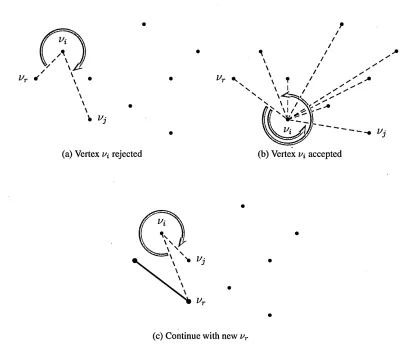
• The point v{ will be considered to belong to the convex hull if the orientation with respect to all other points in Ar is Counter-Clockwise, as shown in Figure 2.7(b), or when it is Collinear with other points that also belong to the convex hull. In the case of collinear points, the one closest to the current reference point is considered first. In this way, all of the points that lie on the convex hull will be included, regardless of whether the points are vertices of the polygon or not.
[image:41.612.191.377.65.200.2]• This process continues until the next point found to be inserted into the convex hull is equal to the first point used as a reference point. At that moment the curve has been closed, and all the remaining points are inside of the convex hull. The program stops evaluating any more points when this condition is reached, otherwise it would continue and produce spiral-like open curves that include all the points in the sample.
Figure 2.7: Selection of vertices belonging to the convex hull of a dataset, based on orientation.
2.3 Notions related to the concept of curvature
2.3.1 Formulae and definitions
The definition of the curvature of a curve is in general given under the assumption that the curve is of C2-class, so that the 1st and 2nd derivatives are continuous. However, the
notion of curvature can be generalised to the class of curves which possess continuous second derivatives except at a finite number of points where a jump discontinuity in the first derivative can occur. Such a curve can be seen as the sum of a finite number of
(a) Vertex Vi rejected (b) Vertex i>i accepted
(c) Continue with new vr
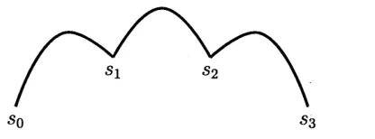
C'2-curves, joined together at n discontinuity points s0, s i , . . . , sn. Figure 2.8 shows a diagram of a curve of this kind.
Figure 2.8: A curve with discontinuity points si and S2.
We can introduce the exterior angle a(si) formed by the right and left tangents at a point of discontinuity s{ (van Rooij 1965). The total curvature o of the curve is then defined as the sum of the integral curvatures k(s) of the smooth segments, plus the sum of the exterior angles at all discontinuity points. We then have the following formula for the curvature of an open curve:
where X) a (si) is the sum of all exterior angles enclosed by the right and left tangents at points of discontinuities between s0 and sn.
In the case of a discrete curve the points of discontinuity are its vertices, while the smooth curves are straight line segments that have curvature equal to zero. (Sullivan 2006) gives a description of some properties of curvature and the relationship between the smooth and discrete cases. We then have that for the discrete case the curvature is reduced to the sum of the angles at the vertices. Let us denote with a(z^) the exterior angle at the vertex i\ of a curve. Then the expression
represents the total curvature of a closed polygonal curve. If this curve is the boundary of a closed simple polygon, u is always equal to 2n (an elementary case of the Gauss-Bonnet theorem). The following expression:
is called the Total Absolute Curvature of a curve, abbreviated as the TAC. An important fact is that Cj reaches its minimum value 27t on convex curves (polygons). We can show this by using a rectangle, as depicted on Figure 2.9. The angles in each of its four vertices (2.3.1)
n
(2.3.2)
n
Figure 2.9: The TAC of a convex curve is always equal to 27r.
The convex hull of any curve is by definition a convex curve, and thus has a curvature equal to 2tt. Any concave vertex in the curve will increase the TAC and make it larger
than 27r. So we have that for any given simple closed curve the following hold: n
uj = ^>2 a^Vi) = 2ir (2.3.4)
i=l
and: n
u) = ^ 2 H " i)\ > 27t. (2.3.5)
2—1
Therefore for a non-convex curve the excess in the Total Absolute Curvature with respect to 27t can be used as a measure of deviation from the convex curve. Given the dataset V , we take as a convex curve o f reference the boundary of the convex hull of the data, (referred to as the CH-curve).
Definition 2.3.1. We call a deviation region or simply a deviation the connected vertices and edges of a curve P (V ) that do not belong to the convex hull of the dataset V . Every deviation is connected to the convex hull at both of its ends, at what we call deviation vertices.
We want to determine the measure of curvature added to a curve P (V ) by its devia tions with respect to the CH-curve. For the problem of curve reconstruction, if our aim is to generate curves of minimum curvature, it is clear that we should minimise the amount of curvature contributed by reflex vertices. Let us make this assumption more precise.
It is possible for a discrete curve to have self-intersections, but in this chapter we presume that polygonal curves represent boundaries of simple polygons, i.e. are not self-intersecting. Furthermore we consider a simple polygonal curve P (V ) as a set of line
segments TWi+i that join the vertices Vi, i/2, . . . , vn-15 vn in a specific order. We consider only closed curves, therefore the line segment belongs to the curve P (V ). For each individual vertex we define:
Definition 2.3.2. The star of a vertex in a curve is the union of the vertex and its two adjacent line segments and 1^ + 1.
In the following explanations of the measurement of the Total Absolute Curvature we will consider the absolute values of all the angles, both convex and concave (reflex). We designate the vertices that lie on the CH-curve with V c h > and with 7iti =
1
, . . . , qthe exterior angles at these vertices with respect to the CH-curve. It is clear thatLet us denote with V COnv the convex vertices of P (V ) and with otj,j =
1
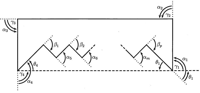
, . . . , r the exterior angles at these vertices with respect to P (V ), and with V reflex the reflex vertices of P (V ) and with /3k, k = 1 , . . . , 5, the corresponding exterior angles at these vertices with respect to P (V ); where r + s = n. Figure 2.10 shows the location of these vertices in a polygon. [image:45.612.87.506.347.543.2](2.3.6)
Figure 2.10: General case with several convex and concave angles.
For a simple closed polygon the following equality holds:
r s
OLj - > p k = 2tt. (2.3.7)
j=i fc=i
The set of convex vertices V COnv can be further split into three disjoint subsets, namely, the subset V COn v - C H of vertices that lie on the CH-curve and such that their stars also belong to the CH-curve; the subset V conv-int of vertices that are convex but do not belong to the CH-curve; and the subset V conv_dev of vertices that lie on the CH - curve but their stars do not belong to the CH-curve. Vertices of the last type are called
deviation vertices as at these vertices the curve is deviated from the CH-curve. The cor responding exterior angles are denoted as a f H, I = 1 , . .. , t, a™1, m = 1 , . . . , u and apev, V — 1> • • • 5v * respectively. We also have that l + m + p = r. Obviously, any part of the curve that is deviated from the CH-curve starts and ends at the neighbouring vertices of V COnv—devj since our curve has no self-intersections. Segments that have a deviation vertex as an end-vertex, but do not belong to the CH-curve, are called deviating segments.
Therefore, Equation 2.3.7 can be rewritten as:
t U V s
X “ f " + £ <*£* + £ - £ > = 2tt. (2.3.9)
1=1 m= 1 p= 1 k= 1
Each ctpev is equal to + 6P\ where by 6P we denote the angle at a deviation vertex
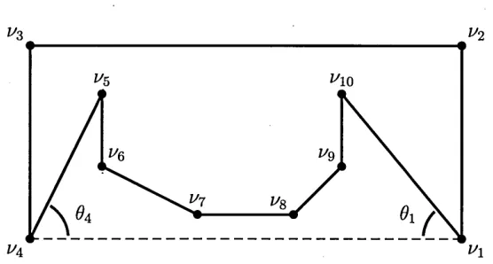
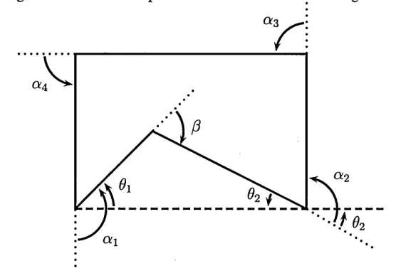
[image:46.612.147.425.428.577.2]of the curve P (V ) with respect to the CH-curve, or in other words, the angle between the deviating segment of P (V ) that has this deviation vertex as one of the end-vertices and the (imaginary) segment of the CH-curve, that would have the same deviation vertex as one of the end-vertices. We call such an angle a deviating angle, as illustrated in Figure 2.11.
Figure 2.11: Deviation angles in a non-convex curve. The deviating angle at vertex is formed by the deviating segment P4P5 and the (imaginary) segment P4F1 belonging to the CH-curve. At vertex v\ the deviation angle is formed by segments F4F1 and viViq.
The above-mentioned considerations transform Equation 2.3.9 into the following one:
t U V V s
£ a f " + £ < ‘ + £ 7 p + I > f - - £ & = 2,r- (2.3.10) 1=1 m = 1 p = 1 p= 1 k= 1
The sum Y?i=i a ?H + S p = i Ip can be rewritten as Yli=i 7* and, as sh