IDRC photo: N. McKee
P M M A W o r k i n g p a p e r
2 0 0 7 - 2 1
Multi-Dimensional Analysis of
Poverty in Ghana Using Fuzzy
Sets Theory
Kojo Appiah-Kubi
Edward Amanning-Ampomah
Christian Ahortor
July 2007
Kojo Appiah-Kubi (University of Ghana)
Edward Amanning-Ampomah (University of Ghana))
Christian Ahortor (University of Ghana)
Abstract
The paper studies the multidimensional aspects of poverty and living conditions in Ghana. The aim is to fill the vacuum that has been left by traditional uni-dimensional measures of deprivation based on poverty lines, exclusively estimated on the basis of monetary variables such as income or consumption expenditure. It combines monetary and non-monetary, and qualitative and quantitative indicators, including housing conditions, the possession of durable goods, equivalent disposable income, and equivalent expenditure, with a number of composite human welfare measures. The study employs the fuzzy-set theoretic framework to compare levels of deprivation in Ghana over time using micro data from the last two rounds of the Ghana Living Standard Surveys (1991/1992 and 1998/1999). The estimation results of the membership functions, depicting the levels of deprivation for the various categories of deprivation indicators, show a composite deprivation degree of 0.2137 for the whole country in 1998/99 as compared to 0.2123 in 1991/92. This deprivation trend reveals that poverty levels had scarcely changed in Ghana. In fact, it even rose slightly during the nineties, contrary to the uni-dimensional analytical GLSS 4 report of an overall broadly favourable trend in poverty in Ghana during the 1990s.
Keywords : Ghana, fuzzy set, multi-dimensional poverty, composite deprivation or poverty index,
1. Introduction
Poverty, as a serious problem in most developing countries, has attracted a lot of attention among analysts in Ghana during the last decade. The country can therefore boast of several reports on poverty trends, i.e. changes in the incidence, depth, and severity of poverty over time (Boateng et al. 2000; Canagarajah et al. 1998, Seini et al. 1997; Asenso-Okyere et al, 1997; Boateng et al. 1992; Glewwe and Twum-Baah, 1991). However, most of these studies have tended to focus on poverty at a point in time, and their analytical methods have usually suffered from a uni-dimensional limitation (Filippone et al 2001), where they referred to only a unique proxy of poverty, namely equivalent income or consumption1. They have also shared the traditional need to dichotomise the population into the poor and the non poor by means of the so called poverty line. While this reductionism simplifies the analysis, as argued by Cheli (1995), it all but wipes out the complexity and multidimensionality of this phenomenon.
Thus in the view of Satterthwaite (2001) uni-dimensional poverty measures, at best, can lead to only a partial understanding of poverty, and often to unfocused or ineffective poverty reduction programs. They fail to capture many aspects of deprivation, including lack of access to the services essential for health and literacy, as well as a lack of political voice and legal protection. Consequently the policy recommendations from such traditional analysis only dwell on transfer policies that alleviate poverty in the short-term (Fusco 2003), while leaving untouched the structural socio-economic policies that could instead break the inter-generational reproduction mechanism of poverty in the long-term (Dagum 2002). These limitations of uni-dimensional poverty measures are also compounded by other technical difficulties of income measurement, especially in developing countries that reduce the value of such income-based uni-dimensional poverty results2.
All these give indications of serious limitations to poverty measures based on a single monetary indicator of resources (Atkinson and Bourguignon 1982, Maasoumi 1998) and underscore the strong need for a multidimensional approach to poverty analysis that widens the concept of poverty to reflect, for instance, dimensions other than just the monetary one. It is believed that the inclusion of other non-market dimensions in normative poverty analysis would help to reveal complexities and ambiguities in the distribution of well-being that income-based poverty analysis cannot capture (Robeyns 2003). This can also facilitate analysts to describe the household’s life-style and thereby go deeper into the meaning and nature of poverty, thus considering poverty in a more modern light, as deprivation that people suffer throughout their lives3 (Pochun 2002). Such a definition may make it possible to differentiate
1
In the view of Maasoumi (1998) such limitation tends to make the meaning of “income” poverty or inequality ambiguous since households and individuals are known to have different characteristics and needs (Maasoumi 1999; 1986). Moreover, it is difficult to have meaningful conceptualization of “income inequality” because of life-cycle differences in incomes, in addition to the fact that not all (non-monetizable or non-tradable) benefits that affect well being have income dimensions.
2
As noted by Sahn and Stifel (1999), the vast majority of African countries, for instance, suffer from paucity of data, which makes it almost impossible to make inter-temporal comparisons of poverty. And where survey data are available at more than one point in time, the determination of changes has proven problematic. This may be due to changes in survey designs and a lack of reliable deflators such as consumer price indices, resulting from serious weaknesses in data collection and related analytical procedures.
3 It must be mentioned that other opinions hold poverty to go beyond the basic needs perspective of
economic well-being (i.e. increased material prosperity) from human well-being (Baliamoune 2003) along the lines of Sen’s notion of functionings and capability4.
In Ghana very little work has been done hitherto by way of analysing poverty in a multi-dimensional sense. This can partly be attributed to paucity of data and lack of reliable deflators, which make it almost impossible to make inter-temporal comparisons of poverty (Sahn and Stifel 1999). Apart from the UNDP Human Development Index (HDI), the only multi-dimensional poverty analysis in Ghana known to the writers is the attempt by Sahn and Stifel (1999) to construct a welfare index for some nine African countries and provide evidence of declining poverty in most of the studied African countries5. Even though their approach successfully reduces the potential arbitrariness of deciding the threshold values (as in the traditional approach) and weights for the resource index6, the results lead to unrealistically large weights being assigned to ownership of certain assets like television and radio, and low weights to more valuable assets like vehicles and other means of transport7.
The aim of this paper therefore is to fill the vacuum that has been left over by the traditional measures of deprivation based on poverty lines, exclusively estimated on the basis of monetary variables such as income or consumption expenditure. It purports to assess living conditions in Ghana with the help of several quantitative and qualitative variables on actual living conditions. These include housing conditions, the possession of durable goods, equivalent disposable income and expenditure. The objective is to provide a more complete picture of poverty, which is closer to what is perceived by just observing reality, than the use of one common indicator such as disposable income or expenditure. Such multidimensional summary measures, decomposed variously as the basic needs indicators, similar to those produced by Brazil8, can be used for effective cross section and inter-temporal poverty comparisons and for geographical poverty mappings. Similarly they can be used to rank geographical areas of the country according to their level of welfare for better policy targeting. The analysis on poverty has basically ranged its methodological choices from descriptive statistics to multivariate methods of factor analysis (Sahn and Stifel 1999; Lelli 2001). But if we side with Cheli (1995) in that poverty is not a discrete attribute characterised in terms of presence or absence, but rather a vague (fuzzy) predicate that manifests itself in different shades and degrees, then a methodological framework that uses fuzzy-sets theory to
minimum level of human self-esteem, including participation in community life and governance (UNDP 1997). The World Bank (1990, 2001), for instance, broadens the notion of poverty to include other forms of deprivation such as vulnerability and exposure to risk—and voicelessness and powerlessness.
4
Functionings refer to various doings and beings of a person, the achievements of an individual determined by the particular way in which he is able to “let the available goods function”. Capability, on the other hand, portrays one’s freedom to choose what kind of life to live and, therefore the actual autonomy in pursuing and achieving those doings and beings one deems valuable (Lelli 2001).
5 Their attempt used data sets from Demographic and Heath Surveys of some 9 African countries and
employed factor analysis of various household characteristics and durables.
6 They allow the data to determine the weights for each asset included in the analysis using factor
analysis and imposing a structure on the variance-covariance of each observed asset (Sahn and Stifel 1999).
7
Moreover, due to data constraints, they confine their chosen variables of welfare to only qualitative indicators and exclude the quantitative element of income, hence the composite index, as an equivalent of full income (Travers and Richardson 1993) fails to give a more complete picture of living conditions of individuals or allow the measure of the volatility of the income with respect to durable goods or housing conditions (Betti
et al. 2000).
analyse poverty may seem appropriate. Fuzzy sets theory has gained popularity in recent times9 because it does not dichotomise the population into poor and non-poor through an arbitrary poverty line like the traditional methods. In this way it is also able to circumscribe targeting errors associated with the drastic differentiation between the poor and the non-poor, particularly between those in similar circumstances but who just happen to lie on opposite sides of a poverty line (Makdissi and Wodon 2004). Hence many analysts including Shorrocks and Subramanian (1994) and Schaich and Munich (1996) have applied it to analyse multi-dimensional poverty (Chiappero Martinetti 1994, 2000).
This study therefore employs the fuzzy-set theoretic framework to compare levels of deprivation in Ghana over time using micro data from the last two rounds of the Ghana Living Standard Surveys (1991 /1992 and 1998/1999). In the context of poverty as a multi-dimensional construct, we attempt here to construct a composite index comprising of several poverty-related indicators, to gauge human deprivation. We also use the factor analytical approach to analyse poverty to determine which methodology gives a better explanation of the poverty situation in Ghana in a multi-dimensional sense.
The rest of the paper is organized as follows: After a brief review of the literature in the next section, we follow up with an overview of the poverty situation in Ghana. The subsequent section presents the methodology for estimating the poverty indices for the various dimensions, to be followed by presentation of the results. A final section presents a summary of the results and concluding remarks.
2. Multi-dimensional Poverty – A Literature Review
The use of indicators to gauge human progress is common and well understood. For a long time, particularly since the introduction of the economic concept of poverty together with that of the poverty line and head count ratio, by Booth (1892) and Rowntree (1901), the reference indicator for poverty has almost always been the equivalent income or consumption. But while these indicators act as reasonably accurate and useful measures of economic performance, and thus can give a workable impression of material well-being, they are by far no precise indicators of poverty.
This has engendered attempts to find appropriate multi-dimensional indicators which can portray the different facets of poverty in any particular country, and in poverty comparisons between countries (Kolm 1977). Also contributing to this increased interest in multidimensional poverty measures is the evolution in conceptual thinking on poverty towards functionings and capabilities as initiated by Amartya Sen’s (1993) well known critique of an income-based analysis of poverty. The consequence is a broadened notion of poverty to include even vulnerability and exposure to risk — and voicelessness and powerlessness (World Bank 2001, 2000) — on the basis that considerations of risk and uncertainty are key to understanding the dynamics leading to and perpetuating poverty (Rosenzweig and Binswanger, 1993; Banerjee and Newman, 1994)10. Hence today poverty is no longer confined to the lack of the ability of
9 See Lemmi and Betti 2006, Barán et al 2006, Makdissi and Wodon 2004, Baliamoune 2004
10 It must be mentioned that other opinions hold poverty to go beyond the basic needs perspective of
people to command sufficient resources to satisfy their basic needs (Piachaud 1987; Townsend 1993) nor considered as a mere economic and monetary dimension, but rather increasingly considered as human deprivation that people suffer throughout their lives. This deprivation in the multi-dimensional sense includes both quantitative and qualitative measures such as the joy of choices, opportunities and others which are most basic to human development and can paint quite different and multi-dimensional pictures of the poverty situation in any particular country, and in poverty comparisons among countries.
The search for suitable ways of measuring multi-dimensional poverty, in the past few decades, has thus led to methodological choices that have been characterised by innovative mixing of quantitative and qualitative methods that address the multi-dimensional nature of poverty and explore poverty dynamics and vulnerability. For this reason there is now a considerable and growing literature on multi-dimensional measures of poverty using several different approaches. These approaches include the social exclusion approach of René Lenoir (1974)11, the work of Townsend (1993, 1979), Sen’s capabilities and functionings approach, and the UNDP Human Poverty Index (1997). Another group includes studies derived from the concept of stochastic dominance, which uses union and intersection approaches to dealing with multidimensional indicators of poverty as developed by Duclos et al. (1999, 2003) as well as other multivariate factor analytical techniques. For instance, Duclos et al. (2003) adapted the stochastic dominance to what can be defined as union, intersection, or intermediate approaches to measure well-being in Uganda in a multi-dimensional sense. Their results revealed regional bivariate poverty comparisons to be similar to univariate comparisons based on expenditures alone, but at odds with univariate comparisons in several ways, comparing results for urban areas in one region with rural areas in another. Even though the poverty orderings seem to be robust to the choice of multidimensional poverty lines and indices, they admittedly concede that the difference in their results obtained from the more complex methods compared with that from the univariate methods do not seem to have been worth the effort. From the literature on multi-dimensional analysis it can be noted that the factor analytical technique has often been used in empirical research in the social sciences for solving the problem of a definite number of well interpretable dimensions of well-being (Lelli 2001; Filmer and Pritchett 2001; Sahn and Stifel 1999). This can be attributed to the ease by which the technique grasps empirical relationships among many different variables12 and the suitability of the technique in situations where there are no reliable household surveys to inform income (or consumption) distribution13. Others have also used different multivariate statistical variants of factorial analysis (Nolan and Whelan, 1996; Layte et al. 2000), principal
minimum level of human self-esteem, including participation in community life and governance (UNDP 1997). The World Bank (1990, 2001), for instance, broadens the notion of poverty to include other forms of deprivation such as vulnerability and exposure to risk—and voicelessness and powerlessness.
11 This was cited from Evans et al (1995).
12 It also facilitates the exploitation of presumed correspondence between the system of latent factors
and the set of observed variables in order to identify the separate dimensions for the given data and determine the extent to which each variable is explained by each dimension. Further fuzzy aggregates, compared with other approaches such as factor analysis, are insensitive to the choice of the form of membership functions (Lelli 2001).
components analysis (Ram 1982; Maasoumi and Nickelsburg 1988; and Maasoumi 1989), cluster analysis (Hirschberg et al. 1991) or latent class model (Pérez-Mayo 2003). Apart from the stochastic dominance approach (Duclos et al. 2003, 1999) mentioned above, recent approaches to multi-dimensional poverty studies have included FGT poverty measures (D’Ambrosio 2005; Foster and Shorrocks 1988; Atkinson 1987) and other multivariate approaches (Dagum 2002; Costa 2003). A particular case of general stochastic conditions is the approach that ranks income distributions where households differ in non-income characteristics, denoted by a discrete variable, and which helps to avoid the use of equivalence scales that are sensitive to assumptions that may not have widespread agreement (Diaz 2003; Dagum 2002). Considering the numerous methods used in analysing poverty and well-being, it appears that there exists a lack of methodological consensus on how multi-dimensional poverty should be measured, despite the limitations of the one-dimensional framework. This leads Qizilbash (2001) to characterise poverty as a vague concept, since there seems to be no clear-cut line between the “poor” and the “non-poor”. Similarly, Mack and Lansley (1985) point out that there is a likely continuum of living standards from the poor to the rich that makes any cut-off point somewhat arbitrary. This calls for a mathematically vague theoretical approach such as fuzzy sets theory, which can also reduce the level of arbitrariness found in ordinary uni-dimensional approaches14.
Of late, this has led to rising interest in the application of the fuzzy sets theory for poverty analysis (Cerioli and Zani (1990); Cheli and Lemmi (1995); Chiappero Martinetti (1994, 2000); Costa (2002, 2003); Dagum (2002); Vero (1999); Miceli (1998)).and Qizilbash (2002), for instance, have applied it to construct poverty measures to explore vulnerability in South Africa. Lelli (2001) has also used it to compare with the results of factor analysis and has found the fuzzy aggregates to be insensitive to the choice of the form of the membership function. Other people have also of late applied it to evaluate living conditions in countries like Italy (Cerioli and Zani 1990), Poland (Cheli et al. 1994) Switzerland (Miceli 1998), South Africa (Qizilbash 2002), and others (see Cheli and Lemmi 1995 or Chiappero-Martinetti 1994, Filipone et al. 2001). Ghellini et al. (1995) for example, have used this methodology to offer a multidimensional and dynamic analysis of deprivation to estimate transition matrices between the deprivation states in the US for the period 1984-1988.
The fuzzy sets theory, despite its increasing application in poverty analysis, has been criticised as ordinal measures, whose values do not have any intrinsic meaning and so put limits both on their interpretability and the possibility of comparing with one another the indices that account for different aspects of poverty. Successive refinements such as the totally fuzzy relative (TFR) proposed by Cheli and Lemmi (1995), have led to alternative specifications of membership functions leading to an expanded interpretability framework of fuzzy indices, and
13
Lelli (2001), for instance, applied factor analysis to measure well-being in Belgium and found that income accounts only for a very limited part of the story and argued for multi-dimensional
approaches like that of Sen (Balimoune 2001) to analyse well-being.
14
It must be pointed out that while this may be true for the headcount ratio setting, the arbitrary choice of a (uni-dimensional and multi-dimensional) poverty line and poverty measure could be addressed using robustness methods or stochastic dominance tests (Duclos et al 2003; Atkinson 1987; Foster and Shorrocks 1988). Moreover, the fuzzy approach is not totally free from arbitrariness
so have made aggregation measures relative to different aspects of poverty less controversial. 2.1 Ghana -- An Overview
Ghana lies on the west coast of Africa, about 5º north of the Equator and is about 238,537 square kilometres in size. It attained independence from British colonial rule in 1957 and became a republic in 1960. It presently has a population of about 20 million people, 40 percent of whom are below 15 years, 3 percent above 65 years and the remaining 57 percent between 16 and 64 years. The population is divided geographically between urban dwellers, which make about 38 percent of the total population and 62 percent rural dwellers. Economically Ghana is a low income country with an estimated per capita income of US$420. Economic growth rates have ranged from 3.3 percent and 5.8 percent over the fifteen-year period 1990-2005. Agriculture contributes the largest share to the gross domestic product (46% in 2004), followed by services (24.3%) and industry (22.1%) (ISSER 2005). In 1983, amid rapidly deteriorating macro-economic indicators, Ghana introduced a World Bank-sponsored Structural Adjustment Programme. This appears to have contributed to some improvements at the macro-economic level. Government domestic revenue as percentage of GDP, for instance, has increased from 6 percent in 1983 to 23.8 percent in 2004. Inflation has also subsided from a high level of 122 percent in 1983 to about 12.8 percent in 2004 (Appiah-Kubi 2003). How-ever, improvements in the country’s international trade and payments situation have been mixed. After the initial improvements in the eighties, the current account balance has remained negative since 1990 due to rapid growth in merchandise imports, while the capital accounts had largely shown a positive balance. This has often led to a negative balance of payment account. However, from year 2000 onwards Ghana has witnessed successive substantial improvement in its balance of payments, with 2003 experiencing a surplus of almost US$600 million (ISSER 2005).
The country has also incurred debts for its development programmes over the years, and owed about US$6.2 million - or the equivalent of 91 percent of its GDP - to external partners as of the end of 2004; this in addition to a huge domestic debt equivalent to 30 percent of GDP at the end of 2003. The burden of this huge indebtedness caused the nation to apply for the IMF’s HIPC facility in 2001. After having successfully passed the decision point in 2002 and the completion point of the programme in 2004, the country was expected to save approximately $230 million (¢2.093 trillion) annually in debt service costs (ISSER 2005).
It is hoped that these relief efforts would go to improve social indicators so as to reduce the prevailing high poverty levels. Even though Ghana has made considerable progress in the overall levels of social indicators, life expectancy at birth continues to linger around 58 years and below the world’s average of 65 years. Infant and under-five mortality rates are still high at 62 and 102 per 1000 births respectively (GDHS 2004). To add, Ghana’s gross primary school enrolment rate of 79 percent is still lower than the average of lower income countries. Only about 44 percent and 31 percent of all Ghanaians are estimated to have access to piped-borne water and sanitation (disposable liquid waste) in their households. All these factors point to the
because since there is no axiomatic basis for justifying the choice of a weighting system under the fuzzy analysis, the results then depend critically on that choice.
endemic nature of poverty in Ghana (ISSER 2005). 2.2 Poverty Analysis in Ghana
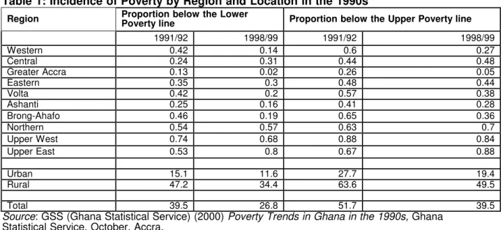
Official estimates of poverty in Ghana have been obtained using consumption expenditure per adult equivalent as the welfare measure (GSS, 2000). Using the traditional uni-dimensional approach to poverty analysis, the Ghana Statistical Service defines two nutrition-based poverty lines viz: an upper poverty line of 900,000 cedis and a lower poverty line of 700,000 cedis per adult per year. While the upper poverty line incorporates both essential food and essential non-food consumption, the lower poverty focuses on what is needed to meet the minimum nutritional requirements of household members. On the basis of the upper poverty line, poverty in Ghana is said to have declined in the 1990s from an estimate of 51.7 percent in 1991/92 to 39.5 percent in 1998/99. Similarly, the proportion of Ghanaians living under extreme poverty, i.e. below the lower poverty line seems to have fallen from 36.5 percent to approximately 27 percent of the total population during the same period. However, the favourable trend in the average masks wide spatial disparities. For instance, the headcount index among rural communities compared to urban communities is higher (Table 1). Extreme poverty is also higher in the country’sthree northern regions, ranging between 57 percent and 80 percent (Table 1) and lower (2%) in the Greater Accra Region. Moreover, the above-mentioned decline in overall poverty level did not occur in all the regions of the country; on the contrary, poverty levels even increased in the 1990s in three regions (Central, Northern and Upper East), two of which (Northern and Upper East) being among the poorest in the country. The above evidence of a general improvement in household welfare had however already been provided by Demery and Squire in 1996. In a study on macro-economic adjustment and poverty in six African countries, they found that the change in poverty in Ghana to reflect the joint impact of a growth in mean income as well as a change in inequality. They also noted that economic growth played a principal role in poverty reduction, particularly between1988-1992.
Table 1: Incidence of Poverty by Region and Location in the 1990s
Source: GSS (Ghana Statistical Service) (2000) Poverty Trends in Ghana in the 1990s, Ghana Statistical Service, October, Accra.
3. Methodology
As stated earlier, the various recent attempts to develop a framework - which allows for the multi-dimensionality, vagueness, and ambiguity of poverty - appear to concentrate on the use of the fuzzy-set theoretic approach (Chiappero Martinetti 1994 and 2000 and Lelli, 2001). The notion of fuzzy-sets was first conceptualised by Zadeh in 1965, (see also 1978) when he defined fuzzy-sets as “a class of objects with a continuum of grades of membership”. This implies that, given some classes of objects do not have precisely defined criteria of membership, it can thus be asserted that these sets do not constitute classes or sets in the usual way in mathematics. Thus the concept of fuzzy sets provides an ideal framework to deal with problems in the absence of a definite criterion for discerning what elements belong or do not belong to a given set. This is particularly the case for solving the problem of identifying the poor in a particular society. With this kind of approach, it is not necessary to specify an arbitrary poverty line as may be required in the case of a head count poverty approach.
For a short mathematical exposition of the fuzzy sets principle, let us consider X as a set and x an element of X. A fuzzy subset P of X can therefore be defined as follows: {x1
µ
P(x)} for all x ∈ X, where µP is a membership function which takes its values in the closed interval [0:1]. Each value µ
P(x) is the degree of membership of x to P.
In a simple application to poverty measurement we can let X be a set of n individuals (i = 1...n) and P, a fuzzy subset of X, the set of poor people. In the fuzzy approach µp(xi), the membership function of the poor set (of individual i) is defined as:
xij= 0, if individual i is absolutely non-poor,
xij= 1, if individual i completely belongs to the poor set, and
0 < xij < 1, if individual i reveals a partial membership to the poor set.
The main issue here therefore is the determination of the individual membership function µp(xi). In its empirical application to poverty Cerioli and Zani (1990) developed a fuzzy theoretical model to multi-dimensional analysis. This was later improved upon by Cheli and
Region Proportion below the Lower Poverty line Proportion below the Upper Poverty line
1991/92 1998/99 1991/92 1998/99 Western 0.42 0.14 0.6 0.27 Central 0.24 0.31 0.44 0.48 Greater Accra 0.13 0.02 0.26 0.05 Eastern 0.35 0.3 0.48 0.44 Volta 0.42 0.2 0.57 0.38 Ashanti 0.25 0.16 0.41 0.28 Brong-Ahafo 0.46 0.19 0.65 0.36 Northern 0.54 0.57 0.63 0.7 Upper West 0.74 0.68 0.88 0.84 Upper East 0.53 0.8 0.67 0.88 Urban 15.1 11.6 27.7 19.4 Rural 47.2 34.4 63.6 49.5 Total 39.5 26.8 51.7 39.5
Lemmi (1995) by deriving the deprivation indices directly from the distribution function of the attributes measured and called this method the Totally Fuzzy and Relative (TFR) method.
Various techniques for the estimation of the membership function have been proposed in the literature. These include the distance and frequency approaches, which may also take the form of (i) quadratic, similar to the sigmoid curve or simply the logistic function, (ii) linear membership function, which is well known and very simple in its application (Lelli 2001). The modalities involved in the selection of a method for estimating the membership function depends upon the ability to identify and specify the variety of variables to which such an indicator may be assigned, as well as the type of variable. Variables can be differentiated into (i) dichotomous or (ii) categorical, which can take on continuous or discrete values. For the aggregation of the indicators in their elementary units (categories) it is appropriate to categorise the steps into two operational stages: (i) the specification of membership for each indicator, and (ii) the specification of the weighting structure.
3.1 Dichotomous variables
Dichotomous variables are those variables whose attributes are defined from the questions of possession or non-possession of durable goods, e.g.: furniture, TV, electrical appliances, etc. The ‘have’ attribute is assumed to have a low risk of deprivation, while the ‘have not’ has a high risk of deprivation. The two attributes have the values of 0 and 1 in the closed set, i.e. [0, 1], whereby 0 takes the low risk of deprivation and 1 takes the high risk of deprivation. Following Costa (2002), upon definition of
i) the set P of poor households;
ii) the degree of membership to the set P of the ai-th household; iii) the deprivation ratio of the ai-th household; and
iv) the deprivation ratio of the population,
we can define the degree of membership to the fuzzy set P of the ai-th household (i=1,...,
n) with respect to the j-th attribute (j=1,..., m) as in equation 1. )) ( ( j i p ij X a x =
µ
(1)Given a population Aof n households, A = {a1, a2, …, an}, µp means membership of the subset of poor households P of which includes any household ai having some degree of poverty in at least one of the m attributes of X. In other words Xj(ai) represents an m-order
vector of socio-economic attributes which will result in the state of poverty of a household ai if partially or not possessed by the household.
In this case:
xij = 1 iff the ai-th household does not possess the j-th attribute.
∑
==
n i in
n
1.
Thus the deprivation index of the ai-th household, µp( )ai (i.e. the degree of membership of the ai-th household to the fuzzy set P), can be defined as the weighted average of xij:
(2)
Whereby wjis the weight attached to the j-th attribute, which stands for the intensity of deprivation of attribute Xj. The weight wj has an inverse relationship with the degree of depriva-tion: the smaller the household population (and the lower the level of deprivation), the greater is the weight wj. This essentially implies that the more an attribute is present in the population,
the fewer the number of households deprived and the more important it becomes. Consequently, such an attribute is likely to attract a greater weight among the attributes included in X. In order to reduce the arbitrariness involved in the estimation of the weights, Cerioli and Zani (1990) propose a logarithmic function, which they define as in equation 3:
where (3)
ni represents the weight attached to each household ai. In the case sample of a survey data, ni is equivalent to n times the relative frequency of households in the total population. It follows that 15 Dagum (2002) specifies the fuzzy poverty index of the population as a weighted average of the poverty ratio of the ai-th household which is stated in equation 4.
(4)
However, if the data is obtained from a random sample or census of households, the weight will be constant and .Thus the poverty ratio of the population could be constructed as in equation 5 (Cerioli and Zani 1990).
(5)
In a further refinement Costa (2002) defines another technique for aggregating the membership degrees into a multi-dimensional composite deprivation or poverty index, which allows the fuzzy set framework to simply obtain a uni-dimensional poverty ratio for each of the j attributes considered. This is in addition to the multi-dimensional poverty ratio of the ai-th household µp( )ai and of the population . In this case the difference between the
multi-dimensional and uni-multi-dimensional poverty ratios lies in the weight. While the multi-multi-dimensional poverty ratio for the ai-th household µp( )ai is the weighted average of xij, with weight wj, the uni-dimensional poverty ratio for the j-th indicator is the weighted average of xij, with weight ni:
(6)
This allows the multi-dimensional poverty ratio of the population as the weighted average of with the weight wj as defined in equation 7.
(7)
15
Equation 3 allows the weight assigned to the jth attribute not to be arbitrarily imposed but to be determined by the sample size and the deprivation index of the ai-th household in respect of the jth
attribute. Other past studies have used other techniques for creating index weights, including giving all items equal weight, using the reciprocal of the proportion of households with the items as a proxy for their relative values (Morris et al. 1999), principal components analysis (Filmer and Pritchett 2001), and factor analysis (Sahn and Stifel 1999).
∑
∑
= ==
m j j m j j ij i pa
x
w
w
1 1/
)
(
µ
∑
= = n i i p p a n 1 ) ( 1 µ µ 0 / log 1 ≥ =∑
= n i i ij j n x n w i n i i p n i i i n i i p p a n n n n a∑
∑
∑
= = = = = 1 1 1 ) ( 1 / ) (µ
µ
µ
n n n n i i i∑
= = 1 / 1 /∑
∑
∑
∑
= = = = = = m j j m j j j p n i i n i i i p p a n n X w w 1 1 1 1 ) ( ) ( µ µ µ∑
∑
= = = n i n i i i ij j p X x n n 1 1 / ) ( µ p µ , ) ( j p X µ.
pµ
Where
µ
p (composite deprivation index) is a monotonic increasing function of the degree of deprivation or poverty of each individual. In this case a deterioration of the living conditions of a subset of the population, other things remaining unchanged, results in an increase in the composite deprivation indexµ
p.The above transformation is done after noting that
(
)
1 1 n j ij pX
nx
µ
=∑
(8)For the estimation of the global overall poverty index P (also for discrete and continuous variables), we apply equation 9 first, which combines the multiple indicators of deprivation at the individual level. In the second step we then aggregate them across individuals into an overall index to satisfy the double decomposability feature (namely subgroup and attribute). This double decomposition is to facilitate the design of inexpensive and efficient programmes for poverty alleviation mainly when financial constraints preclude the elimination of poverty in an entire population segment or by a specific attribute.
[
]
{
(
)
[
(
)
]
}
1 1 j p m j i p n tX
a
P
∑
∑
µ
µ
= ==
(9) 3.2 Discrete Categorical VariablesLike all discrete variables, which may take on only one of a certain number of possible values, e.g. gender or marital status, discrete categorical variables are those with definite and discrete fixed points of values at any given time. Such indicators specifically have linear functions since their values at any given interval can be determined, for example, education. Using basic linear frequency technique16 that is commonly applied in empirical studies and whose extreme values depend exclusively on the variable x17, we shall define the membership function,
µ
y, as an increasing function in equation 10:1 if xij = xmin,j xij - xmin
xmax, j - xmin, j (10)
0 if xij ≥ xmax, j Where:
xmax, j and xmin,j represent the two thresholds (or extreme) values. If the values are
16 An alternative linear approach also mentioned in the literature is the
trapezoidal specification that takes two thresholds a1 and a2 (which are larger than the minimum and smaller than the maximum) with
respect to the variable x. With this approach all the elements of the domain falling within a given set will be given a particular membership function. It is, however, opened to criticism because of its potential arbitrariness. It requires the preliminary definition of two critical values to separate the definitely deprived and the definitely non-deprived, hence lays open to an obvious critique in what concerns the grounds on which the choice of the thresholds takes place. Usually, the subjective beliefs of the researcher performing the analysis represent the rationale for discriminating among the given modalities, thus introducing precise normative assumptions in the whole procedure (Lelli 2001).
17 These, easy to specify, interpret and visualize membership functions, presuppose the variables’
modalities to be equidistant from one another and assume a direct proportionality between the elements of the domain and the membership grade; a very restrictive and not always appropriate assumption (Lelli (2001).
if xmin,j < x <
arranged in increasing order of deprivation, xmin represents the extreme threshold under which
the individual is seen as more deprived in the dimension represented by the indicator j, and xmax, j is the threshold above which an individual is not deprived in the said indicator. The individual i can be said to be partially deprived in cases where xij lies between the two thresholds.
Where there exists a non-linear and monotonic relation between the indicator variable x and the degrees of membership, it is proposed to order the modalities of x with respect to the risk of deprivation k=1,...,K associated to them using the following specification recommended by Cheli and Lemmi (1995)18:
0 if x = xk; k = 1 β(xk) - β(xk-1)
µy = µ(xk-1) + if x = xk; (k > 1) (11) 1 - β(x1)
1 if x = xk; (k = K)
Where β(xk) represents the cumulative distribution of x ranked according to k.
In the view of Lelli (2001) this method offers a way out from the issue of aprioristic choices to intuition by allowing the membership function to be based exclusively on the empirical evidence of the real valued functions of the various categories in each indicator. 3.3 Continuous Categorical Variables
An indicator is said to be continuous categorical if its mass function has no definite or discrete fixed points of values. An obvious example of a quantitative continuous variable is income or expenditure. However, such an indicator can be categorised in stages or in groups such that their relative membership functions can be assigned to each category to allow a general membership function to such indicator to be defined. For ordinal continuous categorical variables, where the frequency associated to one of extreme categories assuming high levels, Filippone et al. (2001) recommend normalised membership fuzzy sets function19 as defined in equation 12.
1 if 0 < yij < ymin,j yij - ymin
ymax, j - ymin, j (12)
0 if yij > ymax, j
Where ymin and ymax stand for the minimum and maximum thresholds that were considered20.
18 This approach of Cheli and Lemmi (1995) is seen to be “relative” inasmuch as the cut-offs and the
way in which membership of the set of the poor varies with an indicator depends on the sampling distribution of the indicator. Further Qizilbash (2001) identifies a high level of multi-dimensionality in the framework.
19 We admit here that even though the estimated poverty results of equation 8 unlike equation 6 violate
the two core axioms of Sen (1976), namely the monotonicity and the transfer axioms, they nonetheless characterise poverty better than the headcount index (in one or many dimensional context).
20
By virtue of the fact that there is no ideal way of setting ymin and ymax without a bit of arbitrariness, we
use the estimated mean expenditure as the ymin and about 60 percent above the mean as the ymax. This
apparently gives an adequate fair distribution of the proportion of the population belonging to the poor and non-poor groups, without revealing any partial membership to a subset.
if ymin,j < yi < ymax, j
Considering income as a continuous variable, we use a synthetic description of the TFR method to derive the membership function defined as follows
H(yi) where the degree of poverty increases with increases in Xj
1 ─ H(yi) otherwise (13)
where (yi) is the equivalent income of household i, H(yi) is the income distribution function and Xj are attributes included in X. This specification derives its theoretical underpinning from the Totally Fuzzy and Relative (TFR) approach developed by Cheli and Lemmi (1995) and is coherent with a relative concept of poverty. It also has an empirical foundation as H(yi) or the income distribution is estimated based on the sample (Cheli 1995). The above function may assume a linearity if the income indicator is categorised, but takes on a non-linear or quadratic membership functional form if it is not categorised because of multiple factors and parameters in such function. An example is the Dagum model (Dagum and Lemmi 1989), which uses maximum likelihood function to estimate the parameters. Theoretically the membership function µ(yi) has the expectation E[yi] = 0.5, therefore E[1-(yi)] is also 0.5. This is a limitation to the model, since it seems to imply that the proportion of the deprived in the subset of household i would always be equal to at least half of the total population or equivalent to the proportion of those who are not deprived. Cheli (1995) therefore recommends attaching an exponential weight, α, to measure the relative weight of the more deprived with respect to the less deprived. This modified version of the membership function is defined in equation 14.
µ(yi)=[1 - (Hyi)]α , α≥1 (14)
The introduction of α exponent essentially serves to obtain poverty indices of the pseudo cardinal type like the head count ratio and the average poverty gap (Betti and Cheli 1998). In practice, equation 14 estimates the individual deprivation index of each household, and aggregating all these values using equation 15 we can obtain a composite index of the overall population.
P = E[µ(y)] = (1/n)∑µ(yi) (15)
4. Data Source
The methodology described above was applied to the data obtained from the third (1991-1992) and fourth (1998-1999) rounds of the Ghana Living Standards Survey (GLSS3 and GLSS4). This is a series of nation-wide household surveys which were conducted by the Ghana Statistical Service with technical assistance from the World Bank. This data source was used due to the lack of a continuous panel or longitudinal data set in Ghana, which should have been the appropriate data source for such a study of poverty dynamics. Ghana currently possesses four rounds of such surveys, which span the period between 1987 and 1999 and which have gained some high measure of reliability over time. The GLSS4 (1999) survey, for instance, includes data collected from about 5,998 households and some 25,000 household members in all the regions of Ghana. The survey contains detailed information on socio-economic and demographic characteristics of every household, including incomes and household expenditure patterns, education, occupational and employment characteristics,
assets and household durable goods, health, and other determinants of household welfare (Glewwe and Twum-Baah, 1991).
Since our study intends to take advantage of the multidimensionality of poverty measures that not only take into account the material situation of individuals but also capture their general living conditions, we shall combine various aspects of poverty as reflected in the above-mentioned socio-economic and demographic characteristics, which give a picture of poverty in the Ghanaian society. Our choice of indicators is based on a so-called welfarist understanding of standard of living, which is based solely on individual preferences or utility. Given the fundamental economic assumption that consumers purchase the best bundle of goods they can afford, the level of expenditure (or consumption) has emerged as a preferred indicator of living standards. But as we know, the expenditure measure of economic welfare ignores such items as non-market goods and non-material human conditions whose value is not translated into consumption behaviour, thus ignoring life-cycle issues (Essama-Nssah 1999). We therefore consider additional non-welfarist indicators such as primary goods (Rawls 1971), resources (Dworkin 1981), opportunities for welfare (Arneson 1989), access to advantage (Cohen 1989, 1990), and capabilities (Sen 1995).
From the numerous variables we select a small set of material and non-material indicators whose changes are assumed to impact on poverty. We classify these indicators, along the lines of Miceli (1998), into categories of indicators comprising the following: housing conditions, living conditions household durable goods, health, economic resources, and capabilities. We reiterate here that the choice of indicators was made by taking into consi-deration factors such as: i) cultural dependence of indicators, ii) temporal dependence, iii) presence of objective elements, and iv)balance between qualitative and quantitative items. A list of the selected indicators is presented in table 2.
Table 2: Categories of Indicators of Deprivation
Housing Conditions Household Durables (Livestock) Living Conditions
Floor Draught Cooking Fuel
Cement Cattle Electricity
Fibre-glass Sheep Gas
Stone Goats Kerosene
Wood Chicken Charcoal
Mud Pigs Wood
Other Others Other
Roof Materials Household Durables Light
Asbestos Furniture Electricity
Cement Refrigerator Generator
Iron Radio and Recorder Kerosene
Wood TV-Video Candles
Thatch Electric Iron Other
Other Car Type of Water
House Wall Living Comfort Indoor plumbing
Cement Number of Rooms Inside standpipe
Stone Economic Resources Water vendor
Corrugated Iron Occupation Status Water truck/tanker service
Wood Equivalent Income Neighbouring household
Mud Equivalent Expenditure (Welfare) Private outside standpipe/tap
Capabilities Clothing Well with pump
Education Footwear Well without pump
None Leisure, culture and Hotels River, lake, spring, pond
Primary Toilet Facilities Rainwater
Secondary Flush toilet Other
Tertiary Pit latrine Water Fetching Comfort
Health Pan/bucket Water distance
Immunisation KVIP
No toilet
A look at table 2 reveals that the selected indicators are mixed categories of dichotomous and continuous types. While most of the household durables are dichotomous variables, equivalent income and expenditure as well as health and distance to water sources are of the continuous type. Education is a discrete categorical variable with a tertiary category being assigned the least deprivation and no education going for the maximum deprivation. The quality of the house occupied by the household as well as living comfort is paramount to the welfare of the members. In this regard poverty ratios related to the type of dwelling, number of rooms and room space, utilities and amenities, as well as the physical characteristics of the dwelling are estimated. The housing conditions are all dichotomous variables, arranged in ascending order of deprivation. Accordingly, households living in houses with mud walls and floors, or with thatch roofing, are assumed to face higher deprivation, while those living in houses with a cement floor and walls, and asbestos roofing are supposed to face lesser deprivation.
The same logic applies to living conditions. Households with electric light are assumed here to face a lesser degree of deprivation than those with candles. Similarly, those enjoying access to water from indoor plumbing are regarded as less deprived than those depending on rivers, ponds, or rainwater as their source of drinking water. In many studies (Miceli 1998; Filippone et al. 2001; Ghellini et al. 1995) size of living space has been used to measure living conditions. In this study, we use the number of rooms available to the household, since rural dwellers can be observed to have large sizes of living space as compared with urban dwellers, but with limited individual comfort. The number of rooms is ranked in ascending order of deprivation with the maximum number of eight rooms being assigned to the less deprived and the minimum number of one room assigned to the deprived in the society.
For the categorisation of the indicators we adapt the suggested approach of Qizilbash (2003). This approach is based on the following plausible (if questionable) method of classifica-tion: if there are n classes in terms of which people or degrees of deprivation are ordered, 1 is the rank order of the class in which everyone is non-poor, and n is the rank order of the class in which everyone is definitely poor. This method of classification means that only the worst off category in each dimension is definitely poor. In the case of education, for instance, someone in the fourth category with no education is definitely poor, while someone in the highest ranked class - i.e. rank order 1 - with a tertiary qualification is non-poor. In the case of distance to water sources, for instance, a household which is less than 5 metres from water has a rank order of 1, and is non-poor, while one which is 500 metres away or more from a water source has rank 5 or 6 respectively and is definitely poor.
Income - represented by the expenditure equivalent proxy - as a measure of deprivation of a decent quality of life rather than the deprivation in the quality of life itself is included in the composite index. Here the continuous indicators of deprivation, income and expenditure (as seen in Table 2) are categorised into three groups in descending order of deprivation21.
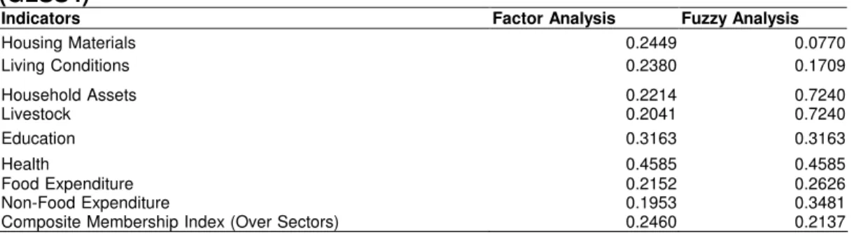
5. Results
The results of the estimation of the membership functions depicting the levels of deprivation for the various categories of deprivation indicators, together with the weights, are presented in table 3. Using data from the latest round of the Ghana Living Standards Survey (1998/99) our study estimates a composite deprivation degree of 0.2137 for the whole country, as compared to the uni-dimensional head count index of 0.395. This means that of Ghanaian households, 21 percent on average registered deprivation on the various wellbeing indicators. It must, however, be noted that the estimated fuzzy normalised proportion of the population suffering deprivation cannot be compared with the head count index of 0.395. Indeed there is no basis for such a comparison since the fuzzy result compensates deprivation in one area from the other. This means that the inability to get certain goods, facilities and opportunities, which are usual in the household environment, can be compensated for with the ability to get others (Pérez-Mayo 2003), whereas the head count is usually based on a single deprivation indicator.
Table 3: Fuzzy deprivation indices (membership functions) for Ghana
1992/93 1998/99 DEPRIVATION INDICATOR MF= µj Weight= ln(1/µj) MF*Weigh t MF=µj Weight= ln(1/µj) MF*Weigh t DIFFERENCE HOUSING CONDITIONS Roofing Materials 0.167 2 1.7883 0.2991 0.1661 1.7953 0.2982 Flooring Materials 0.033 0 3.4120 0.1125 0.0250 3.6872 0.0923 Wall Materials 0.1086 2.2199 0.2411 0.0901 2.4073 0.2168 Total 7.4201 0.6527 7.8898 0.6073 SECTORAL MF 0.0880 2.4308 0.2138 0.0770 2.5643 0.1974 -0.0110 LIVING CONDITIONS Cooking Fuel 0.175 4 1.7407 0.3053 0.1718 1.7613 0.3026 Light 0.206 7 1.5764 0.3259 0.1340 2.0101 0.2693 Water distance 0.147 8 1.9120 0.2826 0.1831 1.6978 0.3108 Type of Water 0.0852 2.4633 0.2098 0.0862 2.4506 0.2113 Nr of Rooms 0.2682 1.3162 0.3529 0.3150 1.1550 0.3639 Toilet 0.2342 1.4515 0.3400 0.2351 1.4476 0.3404 Total 10.4601 1.8164 10.5224 1.7984 SECTORAL MF 0.173 7 1.7507 0.3040 0.1709 1.7666 0.3019 -0.0027 CAPABILITY Education 0.3021 1.1970 0.3616 0.3163 1.1511 0.3641 Health 0.3965 0.9251 0.3668 0.4585 0.7799 0.3575
21 For the related equivalent expenditure it was simply decided to fix the minimum category at about 64
Total 2.1221 0.7284 1.9310 0.7216 SECTORAL MF 0.343 3 1.0693 0.3670 0.3737 0.9843 0.3678 0.0305 HOUSEHOLD ASSETS Household Durables 0.614 2 0.4875 0.2994 0.6807 0.3847 0.2618 Livestock 0.7229 0.3245 0.2346 0.7976 0.2261 0.1803 Total 0.8119 0.5340 0.6107 0.4422 SECTORAL MF 0.6576 0.4191 0.2756 0.7240 0.3230 0.2338 0.0663 HOUSEHOLD EXPENDITURE / WELFARE
Food Expenditure 0.248 3 1.3933 0.3459 0.2626 1.3373 0.3511 Non-Food Expenditure 0.237 1 1.4391 0.3413 0.3481 1.0553 0.3673 Total 2.8324 0.6872 2.3926 0.7185 SECTORAL MF 0.2426 1.4163 0.3436 0.3003 1.2030 0.3612 0.0577 COMPOSITE MEMBERSHIP INDEX* 0.212 3 0.2137 0.0015
* The composite membership index is obtained by first adding the various sectoral MF*Weights and dividing this by the sum of sectoral weights.
The levels of deprivation as reflected in the degrees of membership function differ widely from deprivation characteristic to characteristic, with 0.0770 and 0.7240 as the minimum and maximum respectively, considering quality of housing conditions and household durables as indicator characteristics of deprivation. For example, table 3 reveals a very low average degree of deprivation for floor quality (0.0330). However, this should come as no surprise, given that more than 85 percent of the sampled population of houses has cement floors. On the other hand the table reveals high membership deprivation degrees with respect to household durable goods ranging from 0.6807 to 0.7976 for household durable items and agricultural livestock, respectively.
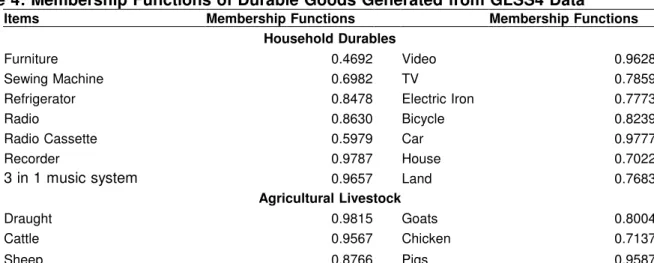
These high deprivation measures (see Table 4) reflect the fact that seemingly “non-essential” household items such as televisions, refrigerators, electric irons, sewing machines, cars, video machines, and others are not so widespread in Ghana. On the average less than about 20 percent of the population were estimated to possess these durable goods. For example, almost 56 percent of the surveyed Ghanaians do not possess household durables assets such as television (57%), radio (52%), refrigerator (65%), fan (54%), car (63%), sewing machine (43%), etc. This evidence, however, stands in sharp contrast with the situation prevailing in most European countries, where these items are regarded as necessities. In his fuzzy poverty study of Switzerland, for example, Miceli (1998) found that a very low proportion (2.5%) of Swiss households was deprived of these items. A little surprising is the high deprivation membership measures for agricultural livestock. Since Ghana, as a developing country, is highly dependent on agriculture, it should be expected to have a lot of livestock. As can be seen in table 4 however, it appears that a sizeable portion of Ghanaians do not keep household farm animals such as sheep, cattle, pigs, etc.
A close look at the degrees of deprivation as reflected in the various membership functions for the various poverty indicators shows a lifestyle among Ghanaians geared toward fulfilling basic necessities. This is manifested in the low deprivation degrees for housing, food, clothing and living conditions. As far as living conditions are concerned, it appears that
Ghanaians have little problem with potable water, since only about 8.6 percent of households do not seem to possess potable water. However, the distance to water sources seems to pose some problems for households. About 18 percent seem to travel long distances to fetch water, and indeed the survey data indicates that over 50 percent of the population travel at least about half a kilometre to fetch potable water.
Table 4: Membership Functions of Durable Goods Generated from GLSS4 Data
Items Membership Functions Membership Functions Household Durables
Furniture 0.4692 Video 0.9628
Sewing Machine 0.6982 TV 0.7859
Refrigerator 0.8478 Electric Iron 0.7773
Radio 0.8630 Bicycle 0.8239
Radio Cassette 0.5979 Car 0.9777
Recorder 0.9787 House 0.7022
3 in 1 music system 0.9657 Land 0.7683
Agricultural Livestock
Draught 0.9815 Goats 0.8004
Cattle 0.9567 Chicken 0.7137
Sheep 0.8766 Pigs 0.9587
With regard to indicators related to equivalent income and expenditure Miceli (1998) cautions on the interpretation of the fuzzy proportion of poor households. Here the membership function is considered along the lines of the average position of households in relation to two extremes, the most deprived and that of the well to do. A look at table 3 above shows that equivalent expenditure was, on average, closer to the bottom end of the distribution in 1998/99. It appears that, while intensity of deprivation seemed to be lower for food expenditures, non-food expenditure was quite high over the same period.
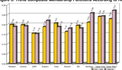
6. Deprivation Trends
In this section we attempt to present poverty patterns and trends using estimates of fuzzy sets theoretic membership functions. We compare GLSS4 data from the 1998/ 1999 survey with that from the previous round (GLSS3) in 1991/1992, which provides an opportunity to trace trends in household deprivation levels or well being over the decade. Even though this study attempts to compare deprivation measures derived from the fourth round with those from the third round and thereby reveal variations in living conditions in the 1990s, we must sound a note of caution that the results reported here are not strictly comparable. This is partly because the use of cross sectional data sets for the analysis gives little insight to poverty dynamics in Ghana22, i.e. investigating the welfare movements of particular households or individuals over time. Moreover, analysis of trends in certain household indicator characteristics is complicated by the fact that the questionnaires for the two surveys are not totally the same. While it was possible to adjust for some of these inconsistencies, it was not possible to correct all of them. Caution therefore has to be exercised in interpreting the trend data.
This constraint notwithstanding, a cursory comparison of the results from the last two rounds of the GLSS, as presented in table 3 above, indicates that deprivation trends have witnessed scarcely any change in Ghana. The results even suggest a slight deterioration in the deprivation trends from 0.2123 in 1991/1992 to 0.2137 in 1998/1999. This appears contrary to the findings of the Ghana Statistical Service, which reports, on the basis of a uni-dimensional income poverty analysis, an overall broadly favourable trend in poverty in Ghana during the 1990s (GSS 2000).
However, there are some differences in the degree of the membership functions or deprivation over time with respect to the various household characteristics. During the nineties, for instance, our results show an improvement in the membership functions with respect to membership functions for household housing characteristics. The respective proportions of the households assumed to be deprived, given certain housing characteristics like roofing, floor and wall materials declined, showed an overall decline in the sectoral membership function from 0.088 in 1991/1992 to 0.077 in 1998/1999. A similar decline can also be observed for living conditions, albeit slight, during the same period (see Table 3). The membership function for light, i.e., the proportion of the population regarded as deprived of electricity, for instance, declined from 0.2067 in 1991/1992 to 0.1340 in 1998/1999.
These findings seem to be confirmed by other survey reports covering the same period. For instance, apart from the GLSS4 report (2000), the GDHS (2004), also reports a 40 percent increase in the use of electricity during the second half of the nineties. On the other hand the trend of the membership functions for household conditions covering capability, assets, and expenditure characteristics experienced various degrees of deterioration. The membership function for the capability characteristic, i.e. the proportion of households deprived of proper health and education, for instance, increased from 0.3433 in 1991/1992 to 0.3737 in 1998/1999, whereas that of household durable assets and expenditure characteristics increased from 0.6576 to 0.7240 and 0.2426 to 0.3003 respectively during the same period. In the case of health the increase in the deprivation levels in Ghana seems to be confirmed by the latest round of data from the Ghana Demographic and Health Survey (GDHS 2004), which reports a decline in vaccination ratios, indicators used as proxy for the health characteristic for the study.
Information on the trends of membership functions or proportion of households owning different consumer durable characteristics in 1991-1992 and 1998-1999 is presented in figures 1 and 2 according to geographical location. We observe in both periods that membership functions are substantially higher in rural areas than urban areas, thus supporting the widely held view that poverty in Ghana is disproportionately a rural phenomenon. We also observe from both figures 1 and 2 that the urban centres seem to have suffered increasing deprivation trends in almost all the identified characteristics as compared to the rural areas, this being especially noticeable for housing and living characteristics. For instance, during the nineties the rural areas seem to have experienced an improvement in housing and living characteristics, while the urban areas seem to have shown a decline with respect to these characteristics.
22 See Appiah-Kubi and others (2004) for attempts at using cross sectional data sets to analyse
Fig. 1 Trends of Membership Functions Urban Fig. 2 Trends of Membership Functions, Rural 0.00 0.10 0.20 0.30 0.40 0.50 0.60
HOUSING LIVING
CAPA-BILITY ASSETS EXPEN-DITURE Tot al Characteristics 1991 / 1992 1998 / 1999
In the case of education and health characteristics, which are often labelled “basic needs” and hence seen as complementary to the consumption-based welfare (expenditure) indicator, a close look at figures 1 and 2 reveal sharp increases in the membership functions of the urban population with respect to these basic needs welfare (expenditure) characteristics. This thus indicates a deterioration in living standards of the urban households during the nineties. This finding also stands in contrast to the findings of the GLSS 4, which reports of slight gains in the basic need characteristics of all households in Ghana.
On the other hand it appears that the rural population seems to have made some improvements in their housing and living conditions during the nineties. This is reflected in the decline in the trend membership functions between 1991/1992 and 1998/1999. The results also seem to corroborate that of the GLSS4 (2004) report that the rural areas appear to have experienced a much bigger change in their housing and living conditions. This change is reflected in the increase in the proportion of households with access to improved housing facilities, water, adequate toilet facilities, electricity, etc., during the nineties. The rural areas, however, appear to have experienced an increase in the membership functions or deterioration in welfare with regard to their ownership of various assets and durables.
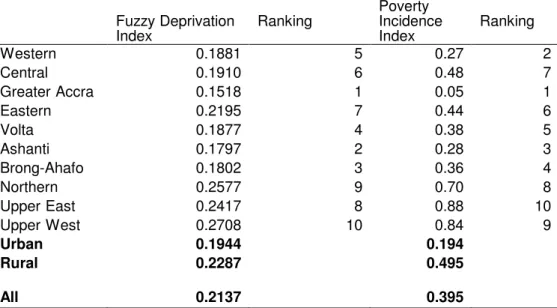
Regional Decomposition of Results
In this section we present some decomposition of deprivation levels with respect to geographical zones in Ghana, which seem to harbour varying degrees of poverty in the various geographical zones. In table 5 we decompose the above-mentioned deprivation levels computed using the 1998/99 round of GLSS according to the administrative regions of Ghana as well as the country’s urban-rural dichotomy. Of all the administrative demarcations in Ghana, the Greater Accra Region has the smallest class of deprived households (about 15.18% of its total households). As would be expected, it ranks first followed by Ashanti Region with a deprivation index of 17.97 percent, while the Upper East Region ranks last as the administrative region with the largest proportion of its households suffering some kind of deprivation. The picture about the regional levels of deprivation is, however, different if one considers the individual categories of deprivation characteristics. With respect to household durables, for instance, the situation concerning the degrees of deprivation is totally the reverse of the usual known order. The three supposedly relatively poor Northern Regions have less proportion of their population living in deprivation as opposed to the other supposedly relatively
0.00 0.10 0.20 0.30 0.40 0.50 0.60
Housing Living Capability Assets Expenditure Total
Characteristics