Lorentz Dispersion Model

Lorentz Dispersion Model

Spectroscopic ellipsometry (SE) is a technique based on the measurement of the relative phase

change of reflected and polarized light in order to characterize thin film optical functions and other

properties. The measured data are used to describe a model where each layer refers to a given

ma-terial. The model uses mathematical relations called dispersion formulae that help to evaluate the

thickness and optical properties of the material by adjusting specific fit parameters.

This application note deals with the Lorentzian dispersion formula.

Note that the technical notes «Classical dispersion model» and «Drude dispersion model» are

com-plementary to this one.

Theoretical model

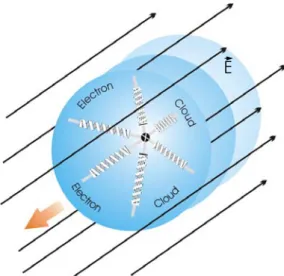
The Lorentz classical theory (1878) is based on the classical theory of interaction between light and matter and is used to describe frequency dependent polariza-tion due to bound charge. The bindings between elec-trons and nucleus are supposed to be similar to the that of a mass-spring system.

Electrons react to an electromagnetic field by vibrating like damped harmonic oscillators. The way the dipole replies to a submitted electric field is given by the fol-lowing equation of motion of a bound electron:

where:

• m d2r/dt2 is the acceleration force;

• mΓ₀ dr/dt is the viscous force; Γ₀ is the damping factor;

• mω_t2r is the Hooke’s force; m is the electronic mass and ω_t is the resonant frequency of the oscillator; • -e E_loc is the local electric field driving force; e is the

magnitude of the electronic charge and Eloc is the

lo-cal electric field acting on the electron. The assump-tion is made that the macroscopic and local electric fields are equal and vary in time as eiωt.

The solution to the previous equation yields the expres-sion for the amplitude of oscillation r depending on the photon energy ω:

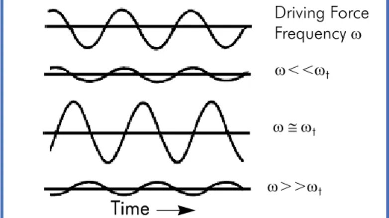
At low frequencies ω<<ω_t, the amplitude r has a me-dium finite value and is in phase with E.

At the resonance frequency ω ≅ ω_t the amplitude is imaginary and maximum when denominator is mini-mum. More, at ω ≅ ω_t there is a 90° phase shift be-tween E and r.

At high frequencies ω>>ω_t, the amplitude r vanishes.

Fig. 1 Restoring force between the orbiting electron and the atomic centre (Ref. 4).

E

( )

1 2 0 2 2 E e r ω m dt r d Γ m dt r d m⋅ r + ⋅ ⋅ r+ ⋅ _t ⋅r=− ⋅ r_loc

( )

1

₍

₎

( )

2 0 2 2

_ω

_ω

ω

ω

⋅ Γ ⋅ + − ⋅ − ⋅ = i E e m r t loc r r

Fig. 2 The oscillator amplitude as a function of frequency (Ref. 5). Phase Amplitude ω<<ω_t ω>>ω_t OSCILLATOR DISPLACEMENT

The induced dipole moment μ is related to r through this relation:

The polarizability α(ω) is given by μ(ω)=α(ω)E(ω) where:

Taking the sum of the single atom dipole moment over all atoms in a volume, it comes that the polarization per unit volume is given by:

The susceptibility χ(ω) is deduced from the previous equation:

squared ω_p2.

The dielectric function is then given through this rela-tion

The limits ε_s and ε_∞ of the dielectric function respec-tively at low and high frequencies are given by:

The complex dielectric function can also be expressed in terms of the constants ε_s and ε_∞ by substituting equations (8) into (7) which yields the following equa-tion:

where ε_s is defined as:

Lorentz model describes radiation absorption due to in-ter-band transitions (quantum-mechanical interpreta-tion). Interband transitions are transitions for which the electron moves to a final state corresponding to a dif-ferent band without changing its k-vector in Brillouin’s first zone.

Extension to multiple oscillators

If there is more than one oscillator, the dielectric func-tion is assumed to be equal to the sum of contribufunc-tions from individual oscillators. This situation fits better to the case of real materials.

In DeltaPsi2 software, the mathematical formulation used for a collection of:

- three Lorentz oscillators is:

- N (N ≥ 1) Lorentz oscillators is:

Increasing the number of oscillators leads to a shift of the peaks of absorption toward the ultraviolet region.

Fig. 3 The response of an oscillator amplitude to a periodic driving force depends on the resonance frequency (Ref 5).

Driving Force Frequency ω ω>>ω_t ω<<ω_t ω ≅ ω_t

Time

( )

( )

( )

_[

₍

₎

_]

( )

3 0 2 2 2

ω

ω

ω

ω

μ

ω

ω

μ

⋅ Γ ⋅ + − ⋅ ⋅ = ⇒ ⋅ − = i m E e r e t loc r r r r

( )

₍

₎

1

( )

4 0 2 2 2

ω

ω

ω

ω

α

⋅ Γ ⋅ + − ⋅ = i m e t

( )

ω

N

α

( ) ( )

ω

E

ω

ε

₀

χ

( ) ( ) ( )

ω

E

ω

5 P = ⋅ ⋅ = ⋅ ⋅

Atom Atom in E-field

r

E

Fig. 4 Polarization of the electronic cloud due to external E-field. (Hecht, Ref. 3)

( )

1

( )

6 0 2 2 0 2

ω

ω

ω

ε

ω

χ

⋅ Γ ⋅ + − ⋅ ⎟⎟ ⎠ ⎞ ⎜⎜ ⎝ ⎛ ⋅ ⋅ = i m e N t

( )

1

( )

1

( )

7 ~ 0 2 2 2

ω

ω

ω

ω

ω

χ

Γ + − + = + = i ω ε t p

(

)

(

)

( )

8 1 ~ 1 0 ~ 2 2 ⎪ ⎩ ⎪ ⎨ ⎧ = ∞ → = + = → = ∞ ε ω ω ε t p s

ε

ω

ω

ε

( )

(

)

( )

9 ~ 0 2 2 2

ω

ω

ω

ω

ε

ε

ε

ω

ε

⋅ Γ ⋅ + − ⋅ − + = ∞ ∞ i t t s 2 2 t p s

_ω

ω

ε

ε

= _∞ +

( )

(

)

_∑

= ∞ ∞ _{− + ⋅ ⋅} ⋅ + ⋅ Γ ⋅ + − ⋅ − + = 2 1 2 2 2 0 0 2 2 2 ~ j oj j j j t t s i f i

ω

ω

γ

ω

ω

ω

ω

ω

ω

ε

ε

ε

ω

ε

( )

_∑

= ∞ _{− + ⋅ ⋅} ⋅ + = N j oj j j j ω γ i ω ω ω f ε ω ε 1 2 2 2 0 ~

The parameters of the equations

4 parameters may be used in the expressions of the single Lorentz oscillator but it may be possible to char-acterize the function with fewer coefficients.

Parameters describing the real part of the dielectric function

• The constant ε_∞ is the high frequency dielectric con-stant; it takes into account the contribution of high energy inter-band transition. Generally, ε_∞=1 but can be greater than 1 if oscillators in higher energies exist and are not taken into account.

• The constant ε_s (ε_s>ε_∞) gives the value of the static dielectric function at a zero frequency. The difference ε_s-ε_∞ represents the strength of the single Lorentz os-cillator. The larger it is then the smaller the width Γ₀ of the peak of the single Lorentz oscillator.

Parameters describing the imaginary part of the sin-gle Lorentz oscillator dielectric function

• ω_t (in eV) is the resonant frequency of the oscillator whose energy corresponds to the absorption peak. When ω_t increases then the peak is shifted to higher photon energies. Generally, 1 ≤ ω_t ≤ 20.

• Γ₀ (in eV) is the broadening of each oscillator also known as the damping factor. The damping effect is due to the absorption process involving transitions between two states. On a graphic representing ε_i(ω), Γ₀ is generally equal to the Full Width At Half Maxi-mum (FWHM) of the peak. As Γ₀ increases the width of the peak increases, but its amplitude decreases. Generally, 0 ≤ Γ₀ ≤ 10.

Parameters describing the imaginary part of the mul-tiple Lorentz oscillators dielectric function.

• fj (j = 1, 2 … N) term is the oscillator strength present in the expression of the multiple Lorentz os-cillator. As fj increases then the peak amplitude in-creases, but the width of the peak γ_j decreases. Generally, 0≤fj≤10.

• ω_0j (in eV) (_j = 1, 2 … N) is the resonant (peak) en-ergy of an oscillator for a collection of several Lorentzian oscillators. It is similar to ω_t. Generally, 1≤ ω_0j≤ 8.

• γ_j (in eV) (j = 1, 2 … N) parameter is the broadening parameter corresponding to the peak energy of each oscillator. It behaves like Γ₀. Generally, 0≤ γ_j≤10.

Limitation of the model

The Lorentz oscillator is not suitable for describing the properties (presence of gap energy and quantum ef-fects) of real absorbing (amorphous, semiconductors) materials.

Parameter set up

Note that:

1. The Lorentzian dielectric function is available in the Classical dispersion formula in the DeltaPsi2 soft-ware.

2. The sign « » before a given parameter means that either the amplitude or the broadening of the peak is linked to that parameter.

3. For each multiple oscillator the graphs show the dif-ferent contributions (in red dashed lines) of the N Lorentzian oscillators to the imaginary part of the Lorentz dielectric function (in red bold line).

> Transparent Lorentz function

- This function exhibits no absorption: Γ₀=0.

- This case corresponds to normal dispersion where ε_r(ω) increases with photon energy.

> Absorbing Lorentz function - This function exhibits absorption: Γ₀≠0.

- The real part of the dielectric function increases with increasing frequency (normal dispersion) except for a region between [3eV - 4eV] where the dispersion be-comes anomalous. The absorption peak is given by the imaginary part of the dielectric function ε_i (ω) and is always positive.

∞

> Multiple oscillator Lorentz function

Applications to materials

The Lorentz oscillator model is applicable to insulators. It describes well for example the behaviour of a trans-parent or weakly absorbent material (insulators, semi-conductors). The spectral range of validity of the Lorentz formula depends on the material but usually the fit is performed over the region ω<ω_t for the single Lorentz oscillator and ω<ω_i in case of multiple oscilla-tors where ω_i is the transition energy of the oscillator of highest order.

List of materials following single lorentz oscillator model

Representation of a Lorentz absorbing function

Dielectric function of CuPc described by 2 oscillators

Dielectric function of a green colored filter described by 4 oscillators

Materials ε? εs ωt Г0 S. R. (eV) AlAs 1.0 8.27 4.519 0.378 0 - 3 AlGaN 1.0 4.6 7.22 0.127 0.6 - 4 AlN 1.0 4.306 8.916 0 0.75 - 4.75 Al2O3 1.0 2.52 12.218 0 0.6 - 6 AlxOy 1.0 3.171 12.866 0.861 0.6 - 6 Aminoacid 1.0 1.486 14.822 0 1.5 - 5 Au disc 1.0 2.409 1.628 0.708 Biofilm 1.0 2.12 12.0 0 1.5 - 5 CaF2 1.0 2.036 15.64 0 0.75 - 4.75 CrO 0.687 3.1 8.0 1.694 Red Color Filter 1.0 2.497 5.278 0 0.65 - 2 GaAs Ox. 2.411 3.186 5.855 0.131 0.75 - 4.75 GeOx 1.0 2.645 16.224 0.463 0.6 - 4 H2O 1.0 1.687 11.38 0 1.5 - 6 HfN 1.0 3.633 8.452 0 HfO2 1.0 2.9 9.4 3.00 1.5 - 6 HMDS 1.0 2.1 12.0 0.500 1.5 - 6.5 ITO 1.0 3.5 6.8 0.637 1.5 - 6 o - LaF3 1.0 2.546 14.098 0.177 0.75 - 4.75 e - LaF3 1.0 2.521 16.842 0.670 0.75 - 4.75 LiGdF4:Eu3+ _{1.0 2.256 16.594 8.416 1,0 - 6.5} LiNbO3 1.0 5.0 12.0 0 LTO 1.0 2.204 13.784 0 MgF2 1.0 1.899 16.691 0 0.8 - 3.8 MgO 11.232 2.599 1.0 0 1.5 - 5.5 NBF3 1.0 2.503 13.911 0 NiO 1.0 121.480 3.470 0.360 ∞ _{εε ∞∞} ε_{s ωt}

List of materials following single Lorentz oscillator

model List of materials following multiple oscillator model

References

1) H. M. Rosenberg, The Solid State, Oxford University Press 2) F. Wooten, Optical Properties of Solids, Academic Press (1972) 3) Eugene Hecht, Optics, Chap. 3, Hardcover (2001)

4) http://www.ifm.liu.se/~boser/surfacemodes/L3.pdf 5) langley.atmos.colostate.edu/at622/notes/at622_sp06_sec13.pdf Materials ε? εs ωt Г0 S. R. (eV) PEI 1.0 2.09 12.0 0 0.75 - 4.75 PEN 1.0 2.466 4.595 0 1.5 - 3.2 PET 1.0 3.2 7.0 0 PMMA 1.0 2.17 11.427 0 0.75 - 4.55 Polycar-bonate 1.0 2.504 12.006 0 1.5 - 4 Polymer 1.0 2.3 12.0 5.0 0.75 - 4.75 PP 1.0 2.16 8.579 0.065 1.5 - 6.5 p-Si 1.0 12.0 4.0 0.5 1.5 - 5 Spincoated Polystryol 1.0 2.25 8.0 0 1.5 - 5 PTFE 1.0 1.7 16.481 0 1.5 - 6.5 PVC 1.0 2.304 12.211 0 1.5 - 4.75 Quartz 1.0 2.264 11.26 0 Resist 1.0 2.189 10.814 0.334 1.5 - 6.5 Sapphire 1.0 3.09 13.259 0 1.5 - 5.5 a-Si : H 3.22 15.53 3.71 2.14 1.5 - 6 a-Si 3.109 17.68 3.93 1.92 1.5 - 6 SiC 3.0 6.8 8.0 0 0.6 - 4 SiN 2.320 3.585 6.495 0.398 0.6 - 6 Si3N4 1.0 5.377 3.186 1.787 1.5 - 5.5 SiO2 1.0 2.12 12.0 0.1 0.7 - 5 SiO2 doped As 1.0 2.154 11.788 0 1.8 - 5 SiOxCHy 1.0 2.099 13.444 0 1.45 - 2.75 SiON 1.0 2.342 10.868 0 0.75 - 3 SnO2 3.156 3.995 4.786 1.236 Ta2O5 1.0 4.133 7.947 0.814 0.75 - 4 TiOx 0.290 3.820 6.50 0 0.6 - 3 YAG:Tb(10%) 1.0 2.545 10.342 0.793 1,0 - 6.5 Y2O3 1.0 2.715 9.093 0 1.55 - 4 ZrO2 1.0 3.829 9.523 0.128 1.5 - 3 ε_s ε_∞ ω_t CuPc Green Color Filter Pentacene/Si e_{∞ 1.800 2.481 1.834} f₁ 0.140 0.00623 1.093 ω0,1 2.000 1.687 1.981 γ1 0.130 0.122 0.207 f2 0.400 0.0170 -1.539* ω_0,2 3.700 1.868 1.982 γ2 0.900 0.127 0.164 f3 0.140 0.00825 0.579 ω0,3 1.700 2.648 1.982 γ3 0.150 0.0717 0.133 f4 0.130 0.0109 1.524 ω_0,4 2.550 2.789 3.100 γ4 0.950 0.162 11.005 Th is do cu me nt i s no t co ntr act ua lly bindi ng under any c ircumstance s - Prin ted in Fr ance - 09/ 200 6 Materials Parameters

ε