econstor
www.econstor.eu
Der Open-Access-Publikationsserver der ZBW – Leibniz-Informationszentrum Wirtschaft The Open Access Publication Server of the ZBW – Leibniz Information Centre for Economics
Nutzungsbedingungen:
Die ZBW räumt Ihnen als Nutzerin/Nutzer das unentgeltliche, räumlich unbeschränkte und zeitlich auf die Dauer des Schutzrechts beschränkte einfache Recht ein, das ausgewählte Werk im Rahmen der unter
→ http://www.econstor.eu/dspace/Nutzungsbedingungen nachzulesenden vollständigen Nutzungsbedingungen zu vervielfältigen, mit denen die Nutzerin/der Nutzer sich durch die erste Nutzung einverstanden erklärt.
Terms of use:
The ZBW grants you, the user, the non-exclusive right to use the selected work free of charge, territorially unrestricted and within the time limit of the term of the property rights according to the terms specified at
→ http://www.econstor.eu/dspace/Nutzungsbedingungen By the first use of the selected work the user agrees and declares to comply with these terms of use.
Badunenko, Oleg; Fritsch, Michael; Stephan, Andreas
Working Paper
Allocative efficiency measurement
revisited: Do we really need input
prices?
The Postgraduate Research Programme working paper series / Europa-Universität Viadrina Frankfurt (Oder), Graduiertenkolleg "Kapitalmärkte und Finanzwirtschaft im erweiterten Europa", No. 2006,7
Provided in cooperation with:
Europa-Universität Viadrina Frankfurt (Oder)
Suggested citation: Badunenko, Oleg; Fritsch, Michael; Stephan, Andreas (2006) : Allocative efficiency measurement revisited: Do we really need input prices?, The Postgraduate Research Programme working paper series / Europa-Universität Viadrina Frankfurt (Oder), Graduiertenkolleg "Kapitalmärkte und Finanzwirtschaft im erweiterten Europa", No. 2006,7, http://hdl.handle.net/10419/22112
Allocative efficiency measurement revisited–
Do we really need input prices?
By Oleg Badunenko, Michael Fritsch and Andreas Stephan∗
January 16, 2006
Abstract
The traditional approach to measuring allocative efficiency is based on input prices, which are rarely known at the firm level. This paper proposes a new approach to measure allocative efficiency which is based on the output-oriented distance to the frontier in a profit–technical efficiency space-and which does not require informa-tion on input prices. To validate the new approach, we perform a Monte-Carlo experiment which provides evidence that the estimates of the new and the tradi-tional approach are highly correlated. Finally, as an illustration, we apply the new approach to a sample of about 900 enterprises from the chemical industry in Ger-many.
JEL Classification: D61, L23, L25, L65
Keywords: allocative efficiency, data envelopment analysis, frontier analysis, tech-nical efficiency, Monte-Carlo study, chemical industry
∗Badunenko, Oleg: (corresponding author) Department of Economics, European University
Vi-adrina; Große Scharrnstr. 59, D-15230, Frankfurt (Oder), Germany,+49(0)33555342946, Fax:
+49(0)33555342959, e-mail: badunenko@uni-ffo.de; Fritsch, Michael: Technical University of Freiberg,
German Institute for Economic Research (DIW Berlin), and Max-Planck Institute of Economics, Jena,
Germany; Lessingstr. 45, D-09596 Freiberg, Germany, e-mail: michael.fritsch@tu-freiberg.de; Stephan,
Andreas: European University Viadrina and German Institute for Economic Research (DIW-Berlin);
1
Introduction
A significant number of empirical studies have investigated the extent and determi-nants of technical efficiency within and across industries (see Alvarez and Crespi 2003,
Caves and Barton 1990, Gumbau-Albert and Joaqu´ın 2002, Green and Mayes 1991, and
Fritsch and Stephan 2004a). Comprehensive literature reviews of the variety of empirical applications are made byLovell 1993andSeiford 1996,1997) Compared to this literature, attempts to quantify the extent and distribution of allocative efficiency are relatively rare (see Greene 1997).1
This is quite surprising since allocative efficiency has traditionally attracted the attention of economists: what is the optimal combination of inputs so that output is produced at minimal cost? How much could the profits be increased by simply reallocating resources? To what extent does competitive pressure reduce the heterogene-ity of allocative inefficiency within industries?2
A firm is said to have realized allocative efficiency if it is operating with the optimal combination of inputs given prices of inputs. The traditional approach to measuring allocative efficiency requires input prices (see
Atkinson and Cornwell 1994, Greene 1997, Kumbhakar 1991, Kumbhakar and Tsionas 2005, and Oum and Zhang 1995) which are hardly available in reality.3
This explains why empirical studies of allocative efficiency are highly concentrated on certain indus-tries, particularly banking, because information on input price can be obtained for these industries.
This paper introduces a new approach to estimating allocative efficiency, which is solely based on quantities and profits and does not require information on input prices. An indicator for allocative efficiency is derived as the output-oriented distance to a frontier in a profit–technical efficiency space. What is, however, needed is an assessment of input-saving technical efficiency; i.e., how less input could be used to produce given outputs.
The paper proceeds as follows: Section 2 theoretically derives a new method for esti-mating allocative efficiency and introduces a theoretical framework for activity analysis models. Section 3 presents the results of the Monte-Carlo experiment on comparison of
allocative efficiency scores calculated using both traditional and new approaches. Sec-tion 4 provides a rationale and a simple illustration using the new approach; Section 5
concludes.
2
Measurement of Allocative Efficiency
2.1
Traditional Approach to Allocative Efficiency
A definition of technical and allocative efficiency was made byFarrell 1957. According to this definition, a firm is technically efficient if it uses the minimal possible combination of inputs for producing a certain output (input orientation). Allocative efficiency, or as Farrell called it price efficiency, refers to the ability of a firm to choose the optimal com-bination of inputs given input prices. If a firm has realized both technical and allocative efficiency, it is then cost efficient (overall efficient).
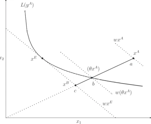
x2 x1 L(yA) xE c b (θxA) w(θxA) wxE wxA xB xA a 6 -s s s s
Figure 1, similarly to Kumbhakar and Lovell 2000, shows firm A producing output
yA represented by the isoquant L(yA). Dotted lines are the isocosts which show level of expenditures for a certain combination of inputs. The slope of the isocosts is equal to the ratio of input prices, w(w1, w2). If the firm is producing output yA with the fac-tor combination xA (a in Figure 1), it is operating technically inefficient. Potentially, it could produce the same output contracting both inputs x1 and x2 (available at prices
w), proportionally (radial approach); the smallest possible contraction is in point b, rep-resenting (θxA) a factor combination. Having reached this point, the firm is considered to be technically efficient. Formally, technical efficiency is measured by the ratio of the current input level to the lowest attainable input level for producing a given amount of output. In terms of Figure 1, technical inefficiency of unit xA is given by
T E(yA, xA) =θ = w(θx A)
wxA (1)
or geometrically by ob/oa. The measure of cost inefficiency (overall efficiency) is given by the ratio of potentially minimal cost to actual cost:
CE(yA, xA, wA) = wxE
wxA (2)
or geometrically by oc/oa. Thus, cost inefficiency is the ratio of expenditures at xE to expenditures at xA while technical efficiency is the ratio of expenditures at (θxA) to expenditures at xA. The remaining portion of the cost efficiency is given by the ratio of expenditures at xE to expenditures at (θxA). It is attributable to the misallocation of inputs given input prices and is known as allocative efficiency:
AE = CE
T E =
wxE/wxA
w(θxA)/wxA (3)
2.2
A New Approach to Allocative Efficiency
When input prices are available, allocative efficiency in the pure Farrell sense can be calcu-lated using, for example, a non-parametric frontier approach F¨are, Grosskopf and Lovell 1994 or a parametric one (Greene 1997, among others). However, if input prices are not available these approaches are not applicable. In contrast to this, the new approach we propose allows measuring allocative efficiency without information on input prices. An estimate of allocative efficiency can be obtained with the new approach that is solely based on information on input and output quantities and on profits.
The first step of this new approach involves the estimation of technical efficiency; whereby, in the second step allocative efficiency is estimated as an output-oriented dis-tance to the frontier in a profit–technical efficiency space.
Proposition 1 Existence of the frontier in profit–technical efficiency space A profit maximum exists for any level of technical efficiency.
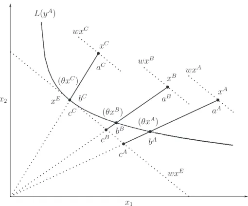
In Figure 2, three firms, A, B, and C using inputs xA, xB and xC, available at prices w,4
produce output yA, which is measured by the isoquant L(yA). For the sake of argument, firms A, B, and C are all equally technically efficient (the level of technical efficiencyθ, however, is arbitrarily chosen) which is read from expenditure levels at (θxA), (θxB), and at (θxC), respectively. In geometrical terms obA/oaA=obB/oaB =obC/oaC. The costs of these three firms are determined by wxA, wxB, and by wxC. The isocost corresponding to expenditures at xC is the closest possible to the origin o for this level of technical efficiency and, therefore, implies the lowest level of cost. This is because xC is the combination of inputs lying on the ray from origin and going through the tangent point of the isocost (corresponding to expenditure level of wxE) to the isoquant L(yA). This implies that forθ-level of technical efficiency costs have a lower bound and using the fact that firms are producing the same output yA, profits have an upper bound. Without loss of generality, for each levelθ of technical efficiency there is a profit maximum, which proves the existence of a frontier in profit–technical efficiency space.
x2 x1 L(yA) xE (θxC) bC cC (θxB) bB cB cA bA (θxA) wxE wxC wxB wxA xC xB xA aC aB aA 6 -s s s s s s s s
Figure 2: Bound of a profit
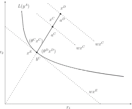
Remark 1 Frontier in profit–technical efficiency space is sloped upwards
In Figure 3, two firms, C and D, use inputs xC and xD to produce output yA, which is measured by the isoquant L(yA). Both firms are allocatively efficient because they lie on the same ray from the origin that goes through the tangent point xE; thus, in terms of Proposition 1 we only look at the frontier points. These firms operate, however, at different levels of technical efficiency θC and θD, respectively. Since the isocost repre-senting the level of expenditure wxC is closer to the origin than that of the expenditure level wxD, costs of firm C are smaller than those of firm D and firm C is more profitable than firm D. Since obC/oaC > obC/oaD, θC > θD, larger technical efficiency is associated with larger profits for points forming the frontier in profit–technical efficiency space. This proves that such frontier is upward sloping.
Proposition 2 The higher the allocative efficiency the higher the profit For any arbitrarily chosen level of technical efficiency, the closer the input combination to the
x2 x1 L(yA) xE (θCxC) (θDxD) bC wxE wxC wx C xC xD aC aD 6 -s s s
Figure 3: Relationship between technical efficiency and profit
optimal one (i.e., the larger the allocative efficiency) the larger the profit will be.
Equation 3 suggests that in terms of Figure 2 (all three firms are equally technically efficient) expenditures solely depend on allocative efficiency. Moreover, the smaller the allocative efficiency the larger the expenditure. Keeping in mind that these firms produce the same output yA, we conclude that for θ-level of technical efficiency (again chosen arbitrarily) the larger the allocative efficiency the lower the costs and the larger the profit is; as allocative efficiency reaches its maximum (for firm C), the maximal profit is also achieved. Without loss of generality, this statement is true for any level of technical efficiency.
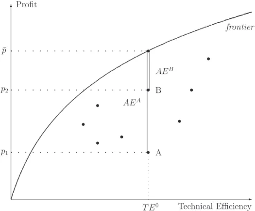
Proposition 3 Allocative efficiency in profit–technical efficiency space Output-oriented distance to the frontier in profit–technical efficiency space measures allocative efficiency.
AEA AEB A B p1 p2 ¯ p T E0 Technical Efficiency Profit frontier 6 -s s s s s s s s s s
Figure 4: Allocative efficiency in profit–technical efficiency space
In Figure 4 frontier is the locus of the maximum attainable profits as defined in Propo-sition 1. The firms A, B, and C have the same technical efficiency level T E0
; however, they have different profit levels: p1, p2, and p, respectively. The potential level of profit
which firms can reach is p. The closer the observation is to the frontier, the larger the profit is. As we recall from Figure2, the shift from firm A to firm C is only possible when the input-mix is changed; i.e., allocative efficiency is improved. Thus, in Figure 4 the shift from firm A to firm B means an increase in allocative efficiency (distance AEA is larger then distance AEB), and further increase in allocative efficiency within the same level of technical efficiency is only possible up to firm Cs observation, for which both profit and allocative efficiency are at the maximum. Thus, which is most remarkable, a vertical distance from the observation to the frontier serves as a measure of the allocative efficiency.
specif-ically, this is the output-oriented distance to the frontier in profit–technical efficiency space.
3
Monte-Carlo simulation
To analyze whether our new approach to measuring allocative efficiency yields valid es-timates, we conducted several Monte-Carlo experiments. According to a micro-economic theory, a firm which chooses such a combination of inputs, that their ratio cost shares is equal to the ratio of output elasticities of the respective inputs, will be most profitable. When we speak of optimal combination of inputs, the original notion of allocative effi-ciency comes into play, and we suggest that the closer the cost share ratio of inputs to the ratio of elasticities the larger a firm’s allocative efficiency will be.
3.1
Empirical implementation of the traditional approach
The traditional approach can be used when input prices are known. Under technologyT
such that
T ={(x, y) can produce y} (4) we measure input-oriented technical efficiency as the greatest proportion that the inputs can be reduced and still produce the same outputs:
Fi(y, x) = inf{λ: λx can still produce y} (5)
We employ the Data Envelopment Analysis (DEA) all the way through the empirical estimation. For K observations, M outputs, and N inputs an estimate of the Farrell Input-Saving Measure of Technical Efficiency can be calculated by solving a linear programming problem for each observation j (j = 1, . . . , K):
d TEj =Fcji(y, x|C) = min ( λ: K X k=1 zkykm ≥yj, K X k=1 zkxkn≤xjλ, zk≥0 ) (6)
for m= 1, . . . , M and n = 1, . . . , N. Note that superscript istands for input orientation while C denotes constant returns-to-scale. Other returns-to-scale are modeled adjusting process operating levels zks (see F¨are and Primont 1995 for details).
When input prices and quantities are given we can calculate the total costs and the minimum attainable cost (solve linear programming problem) and then compute an estimate ofcost efficiency for each observationj (j = 1, . . . , K) as in equation (2):
c Ci j(y, x, w|C) = minnPNn=1wjnxjn: PK k=1z ′ kykm ≥yj, PK k=1z ′ kxkn ≥xj, z ′ k ≥0 o PN n=1wjnxjn (7)
for m = 1, . . . , M and n = 1, . . . , N. We refer to the residual of technical and cost efficiencies as Input Allocative Efficiency, which can be computed for each observation j
(j = 1, . . . , K) as: d AEij(y, x, w|C) = c Ci j(y, x, w|C) c Fi j(y, x|C) (8)
3.2
Empirical implementation of the new approach
As mentioned above, the main virtue of the new approach is that we do not necessarily need input prices for measuring allocative efficiency. Technically, we need output-oriented distances to the frontier in the profit–technical efficiency space. We take advantage of the technical efficiency estimates (denoted by TE) obtained as in equation (6) and profitability measure (denoted by Pr) to calculate (solve linear programming problem) allocative efficiency for each observation j (j = 1, . . . , K) as follows:
d AEij(y, x|C) = max ( θ: K X k=1 zk′′Prk ≥Prjθ, K X k=1 zk′′TEk ≤TEj, z ′′ k ≥0 ) (9)
3.3
Design of the Monte-Carlo experiments
In each of the Monte-Carlo trials, we study a production process which uses two inputs to produce one output. Data for the ith observation in each Monte-Carlo experiment were
generated using the following algorithm.
(i). We chose output elasticities of two inputs to be 0.2 and 0.8. (ii). Draw x1 ∼(φ+λ·uniform); uniform on the interval [0;1].
(iii). Draw r ∼ uniform; uniform on the interval [0;8]. This is meant to be an experi-mental ratio of used inputs.
(iv). Setx2 =rx1.
(v). Choose ǫ. In doing so, we allow the ratio of inputs in each Monte-Carlo trial to vary on the interval [ǫ; 8−ǫ]. Therefore, we obtain enough variation of inefficient combinations of inputs, or in other words, enough variation of allocative inefficiency. (vi). Drawu∼N+
(0, σ2
u) and set ‘te drawn’ equalexp(−u).
(vii). Generate output data assuming trans-log production function, which will contain inefficiency component:5 yi= 0.2x1i+ 0.8x2+γ11x 2 1i+γ22x 2 2i+ 1 2γ12x1ix2i+ te drawni, i= 1, . . . , N (10) The chosen parameter values ensure homogeneity of degree one. We run the simulations with N = 100 and with N = 400.
(viii). Draw price of input x1: w1 ∼(ϕ+ψ·uniform), uniform on the interval [0;1]. The
price of input x2 is calculated as w2 = θw1—we want to keep the ratio of input
prices constant to have the isoquants parallel (recall Figure 2).
(ix). Set profit as output (we set output price equal to 1) minus cost and this is divided by output.
(xi). DEA our measures of allocative efficiency using technical efficiency drawn in step(vi)
as in equation (9).
(xii). Solve for technical efficiency as in equation (6), and DEA our measure of allocative efficiency using these solved technical efficiency scores.
(xiii). Calculate rank correlation coefficient between allocative efficiency estimates based on traditional and our approaches.
(xiv). Repeat steps (i) through(xiii) L times.
In each of our experiments we set φ= 1, λ= 7, ϕ= 1, ψ = 0.05, γ11 = 0.01,γ22= 0.01,
and γ12 = −0.02. In order to look at different variabilities of inappropriately chosen
ratios of inputs, we set ǫ = 0.5, ǫ = 1, and ǫ = 2. With ǫ = 2, variability of allocative efficiency is expected to have been reduced considerably-range becomes [2;6]; and vice versa, ǫ = 0.5 ensures very large variability—range increases to [0.5;7.5]. We conduct three sets of experiments setting σ2
u to 0.0025, 0.025, and 0.25; this ensures covering a plausible range of standard deviations of technical efficiency.6
In each experiment we ran L=500 Monte-Carlo trials.7
3.4
Results
From Tables 1-6 it is clearly seen that in all three cases the DEA estimates the drawn technical efficiency scores fairly accurately—the rank correlation coefficient (Corr4) is close to one. This is an expected outcome since we do not assume a stochastic term in the production output generation (step (vii)of the experiment). The same argument applies to the rank correlation coefficient between allocative efficiency calculated in step(xi)and that calculated in step(xii)(Corr3). Thus, there is not much difference in using the true or the estimated technical efficiency in the new approach. However, what is of most interest to us are the rank correlation coefficients between allocative efficiency estimates from the traditional and our new approach (Corr1 and Corr2). Corr1 has been computed with the
estimates of allocative efficiency based on “true” technical efficiency while Corr2 has been computed with the estimates of allocative efficiency based on estimated values of technical efficiency. As previously mentioned, the rank correlation between these measures is quite high (Corr3). We argue that it is more appropriate to draw conclusions from Corr2 since we do not know the “true” technical efficiency in practice.
The first observation worth mentioning is that when variability of sub-optimal ratios decreases (ǫ increases): our method is less successful in yielding similar estimates as the traditional one. Hence, our method deteriorates in terms of exactness when “true” allocative efficiency is not very heterogeneous.
Furthermore, the results show that our approach is robust with respect to variance of the drawn technical efficiency, σ2
u. Looking closely at correspondent ratios, one can notice that for the same θ’s Corr2 is increasing when σ2
u increases, whereas for other
θ’s Corr2 decreases when we increase σ2
u; however, the changes are minor. The same argument applies to the standard deviation of Corr2. This implies that for different levels of σ2
u distributions of Corr2 are virtually the same. The skewness of the variable Corr2 is always negative and is about –0.6 which means that the distribution of Corr2 is skewed to the left and more values are clustered to the right of the mean. Kurtosis is about 0.6, but it varies more than the skewness; it increases with increase of σ2
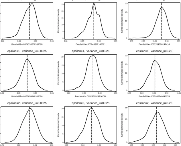
u. Kernel density estimates of Corr2 for the case θ = 0.75 are shown in Figure 5. Note that we use the Gaussian kernel function and the Sheather and Jones 1991 rule to determine the “optimal” bandwidth.
The results are better when the sample size is increased to 400 (Tables 4-6). However, the improvement does not change our main conclusions based on the experiments with sample size 100. As expected, standard deviations of rank coefficients are almost halved when the sample size is quadrupled.
Results of one run8
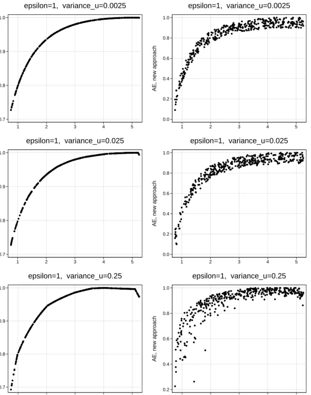
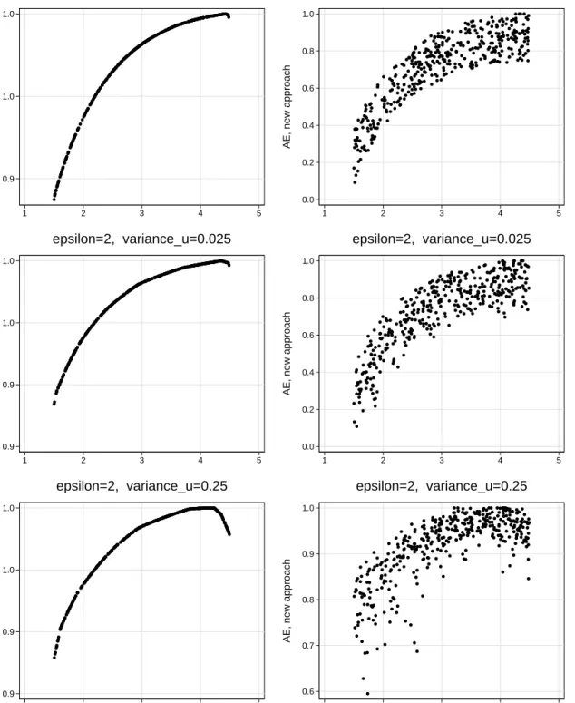
(sample size 500) are summarized in Figure 6. Our methodology almost completely repeats the trend of the traditional approach for ǫ = 0.5 which is backed by a high correlation coefficient in Tables 1 and 4; as ǫ becomes larger Figure 6
suggests that our methodology is less able to predicts allocative efficiency. However, it is most remarkable that our methodology is in line with the traditional approach.
4
Empirical illustration of the new approach
4.1
Data
To illustrate the usefulness of the new approach for measuring allocative efficiency when input prices are not available, we apply it to micro-data from the German Cost Structure Census9
of manufacturing for the year 2003. Our sample comprises only enterprises from the chemical industry. The measure of output is gross production. This mainly consists of the turnover and the net-change of the stock of the final products.10
The Cost Structure Census contains information for a number of input categories.11
These categories are payroll, employers’ contribution to the social security system, fringe benefits, expenditure for material inputs, self-provided equipment, and goods for resale, for energy, for external wage-work, external maintenance and repair, tax depreciation of fixed assets, subsidies, rents and leases, insurance costs, sales tax, other taxes and public fees, interest on outside capital as well as “other” costs such as license fees, bank charges and postage, or expenses for marketing and transport.
Some of the cost categories which include expenditures for external wage-work and external maintenance and repair contain a relatively high share of reported zero values because many firms do not utilize these types of inputs. Such zeros make the firms incomparable and, thus, might bias the DEA results. In order to reduce the number of reported zero input quantities, we aggregated the inputs into the following categories: (i) material inputs (intermediate material consumption plus commodity inputs), (ii) labor compensation (salaries and wages plus employer’s social insurance contributions), (iii) energy consumption, (iv) user cost of capital (depreciation plus rents and leases), (v) external services (e.g., repair costs and external wage-work), and (vi) “other” inputs related to production (e.g., transportation services, consulting, or marketing).
Profits are computed as one minus the total costs divided by the turnover. Since the DEA requires positive values, we standardize the profit measure to the interval (0,1) by adding the minimum profit and dividing this by the range of profits.
4.2
Results
Figure 7 shows profitability plotted against estimated technical efficiency. Remarkably, a frontier, as could be theoretically expected from Proposition 1, indeed exists. Another observation worth mentioning is that within a certain level of technical efficiency (i) prof-itability greatly varies suggesting variation in allocative efficiency (as firms A, B, and C in Proposition3) and (ii) profits are bounded from above. Moreover, the frontier is posi-tively sloped as was stated in the first theoretical part of this paper. Interestingly, Figure 7 suggests that even with 100 percent technical efficiency enterprises can be allocatively inefficient.
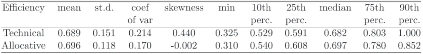
We calculated technical efficiency scores as in equation (6). Table7, which contains de-scriptive statistics of the estimated technical efficiencies, suggests that an average German chemical manufacturing enterprise is fairly inefficient. The median of technical efficiency implies that half of firms have an efficiency of 68 percent or less. The scores for alloca-tive efficiency are obtained solving the linear programming problem as in equation (9). Descriptive statistics on allocative efficiency are also presented in Table 7. At a first glance, the mean and the variation of allocative efficiency appear to be strikingly similar to that of technical efficiency. However, the distribution of allocative efficiency is more symmetric and has a lower variance compared to the technical efficiency distribution.
Kernel estimated density of technical efficiency is shown in the left panel of Figure8; we use Gaussian kernel function and the Sheather and Jones 1991 rule to determine the “optimal” bandwidth. Although the number of firms is quite large, we analyze the sensitivity of efficiency scores relative to the sampling variations of the estimated frontier in an additional step. Consequently, we perform the homogeneous bootstrap as described by Simar and Wilson 1998. The geometric mean of the bias-corrected efficiency scores
is 0.6066, which is on average 0.0886 lower than that estimated via the DEA; the mean variance of bias is 0.0036. In comparison to other studies, however, the bias of estimates and its standard error are rather low, thereby indicating a robustness of the technical efficiency scores.
5
Conclusions
Allocative inefficiency, introduced in the seminal work by Farrell 1957, has important implications from the perspective of the firm. How much could firms increase their profits-given a certain output they produce-just by reallocating resources? On the other hand, the existing empirical evidence on the extent and determinants of allocative efficiency within and across industries is rather limited. The main reason is that the traditional approach to assessing allocative efficiency requires input prices. However, input prices are rarely accessible, whichper se, precludes the analysis of the allocative efficiency with non-parametric approach.
In this paper, a new method is developed which enables calculating allocative efficiency without knowing input prices. This indicator is derived as the output-oriented distance to the frontier in profit–technical efficiency space. Thus, besides input and output quantities, only the profits of the firms are needed for calculating allocative efficiency. A simple Monte-Carlo experiment was performed to check the validity of the new methodology. We obtain high-rank correlation coefficients between allocative efficiency estimates based on both traditional and new approaches for different parameter constellations. Moreover, the new approach proved to be quite robust with respect to variance of true technical efficiency. Finally, we applied the new approach to a sample of about 900 enterprises in the German chemical industry. The results suggest a large variation of allocative efficiency even for technically efficient enterprises. Thus, the example highlights the usefulness of our method for obtaining allocative efficiency measures when input prices are not available.
Endnotes
∗The research on this project has benefited from the comments of participants of the Royal Economic
Society Conference [2005], 3d
International Industrial Organization Conference, 10th
Spring Meeting of Young Economists, and IX European Workshop on Efficiency and Productivity Analysis.
1
For studies in the financial sector, see the review byBerger and Humphrey 1997and alsoTopuz, Darrat and Shelor
2005,F¨are, Grosskopf and Weber 2004,Isik and Hassan 2002. Some studies have been performed for the
agricultural sector (e.g.,Coelli, Rahman and Thirtle 2002,Chavas and Aliber 1993,Chavas, Petrie and Roth
2005, and Grazhdaninova and Zvi 2005). Studies for manufacturing sector are relatively rare (e.g.,
Burki, Khan and Bratsberg 1997, andKim and Gwangho 2001)
2
Moreover, allocative efficiency is also import for the analysis of the production process; e.g., to
estimate the bias of (i) the cost function parameters, (ii) returns to scale, (iii) input price elasticities, and
(iv) cost-inefficiency Kumbhakar and Wang forthcoming or to validate the aggregation of productivity
indexRaa 2005).
3
This includes retrieving allocative efficiency using shadow prices (seeGreene 1997andLovell 1993).
4
Let us assume that the ratios of input prices are equal for each firm. This assumption is needed to have the isocosts parallel to each other.
5
Since the DEA is deterministic, we do not incorporate a stochastic term in the Monte-Carlo trials.
6
Using a different experiment, Greene 2005 obtains estimates of technical efficiency with standard
deviations from 0.09 to 0.43.
7
The simulation is programmed in SAS 9.1.3; computationally, one run with N=100, L=500 takes about 7 hours on a Pentium IV processor running at 3GHz. Thus, we defined relatively few parameter constellations in the performed experiment.
8
We repeated this experiment many times and the general picture was always similar; however, due to space constraints it is not possible to present all results here.
9
Aggregate figures are published annually in Fachserie 4, Reihe 4.3 of Kostenstrukturerhebung im
Verarbeitenden Gewerbe (diverse years). For more details on the Cost Structure Census, see Appendix
A1.
10
We do not include turnover from activities that are classified as miscellaneous such as license fees, commissions, rents, leasing etc. because this kind of revenue cannot adequately be explained by the means of a production function.
11
Though the production theory framework requires real quantities, using expenditures as proxies for
inputs in the production function is quite common in the literature (seee.g.,Paul, Nehring, Banker and Somwaru
References
Alvarez, Roberto and Crespi, Gustavo: 2003, Determinants of technical efficiency in small firms,Small Business Economics 20, 233–244.
Atkinson, Scott E. and Cornwell, Christopher: 1994, Parametric estimation of technical and allocative inefficiency with panel data,International Economic Review35(1), 231– 243.
Berger, Allen N. and Humphrey, David B.: 1997, Efficiency of financial institutions: international survey and directions for future research,European Journal of Operational Research98, 175–212.
Burki, Abid A., Khan, Mushtaq A. and Bratsberg, Bernt: 1997, Parametric tests of allocative efficiency in the manufacturing sectors of India and Pakistan, Applied Eco-nomics29(1), 1–22.
Caves, Richard E. and Barton, David R.: 1990, Efficiency in U.S. manufacturing indus-tries, MIT Press, Cambridge (Mass.).
Chavas, Jean-Paul and Aliber, M.: 1993, An analysis of economic efficiency in agriculture: A nonparametric approach,American Journal of Agricultural Economics 18, 1–16. Chavas, Jean-Paul, Petrie, Ragan and Roth, Michael: 2005, Farm household production
efficiency: Evidence from the Gambia, American Journal of Agricultural Economics
81(1), 160–179.
Coelli, Tim, Rahman, Sanzidur and Thirtle, Colin: 2002, Technical, allocative, cost and scale efficiencies in Bangladesh rice cultivation: A non-parametric approach, Journal of Agricultural Economics53(3), 607–626.
F¨are, Rolf, Grosskopf, Shawna and Lovell, C. A. Knox: 1994, Production Frontiers, Cambridge University Press, Cambridge U.K.
F¨are, Rolf, Grosskopf, Shawna and Weber, William L.: 2004, The effect of risk-based capital requirements on profit efficiency in banking,Applied Economics36, 1731–1743. F¨are, Rolf and Primont, Daniel: 1995,Multi-Output Production and Duality, Theory and
Applications, Kluwer Academic Publishers, Boston.
Farrell, Michael J.: 1957, The measurement of productive efficiency, Journal of the Royal Statistical Society. Series A (General)120(3), 253–290.
Fritsch, Michael and Stephan, Andreas: 2004a, The distribution and heterogeneity of technical efficiency within industries–an empirical assessment, Discussion paper, DIW, Berlin.
G¨orzig, Bernd, Fritsch, Michael, Hennchen, Ottmar and Stephan, Andreas: 2004, Cost structure surveys in Germany,Journal of Applied Social Science Studies124, 557–566. Grazhdaninova, Margarita and Zvi, Lerman: 2005, Allocative and technical efficiency of
corporate farms in Russia, Comparative Economic Studies47(1), 200–213.
Green, Alison and Mayes, David: 1991, Technical inefficiency in manufacturing industries, The Economic Journal 101(406), 523–538.
Greene, William: 1997, Frontier production functions, M. Hashem Pesaran and Pe-ter Schmidt (eds.): Handbook of Applied Econometrics, vol. II, Blackwell Publishers, pp. 81–166.
Greene, William: 2005, Reconsidering heterogeneity in panel data estimators of the stochastic frontier model,Journal of Econometrics126, 269–303.
Gumbau-Albert, Mercedes and Joaqu´ın, Maudos: 2002, The determinants of efficiency: the case of the Spanish industry, Applied Economics 34, 1941–1948.
Isik, Ihsan and Hassan, M. Kabir: 2002, Technical, scale and allocative efficiencies of Turkish banking industry, Journal of Banking and Finance26(4), 719–766.
Kim, Sangho and Gwangho, Han: 2001, A decomposition of total factor productivity growth in Korean manufacturing industries: A stochastic frontier approach,Journal of Productivity Analysis 16(3), 269–281.
Kostenstrukturerhebung im Verarbeitenden Gewerbe: diverse years, German Federal Sta-tistical Office, Stuttgart: Metzler-Poeschel, Fachserie 4, Reihe 4.3.
Kumbhakar, Subal C.: 1991, The measurement and decomposition of cost-inefficiency: The translog cost system,Oxford Economic Papers, New Series 43(4), 667–683. Kumbhakar, Subal C. and Lovell, C.A. Knox: 2000, Stochastic Frontier Analysis,
Cam-bridge University Press.
Kumbhakar, Subal C. and Tsionas, Efthymios G.: 2005, Measuring technical and alloca-tive inefficiency in the translog cost system: a Bayesian approach, Journal of Econo-metrics 126, 355–384.
Kumbhakar, Subal C. and Wang, Hung-Jen: forthcoming, Pitfalls in the estimation of a cost function that ignores allocative inefficiency: A Monte Carlo analysis, Journal of Econometrics .
Lovell, C.A. Knox: 1993, Production frontier and productive efficiency, Harold O. Fried, C.A. Knox Lovell and Shelton S. Schmidt (eds.): The Measurement of Productive Ef-ficiency? Technics and Applications, Oxford University Press, pp. 3–67.
Oum, Tae Hoon and Zhang, Yimin: 1995, Competition and allocative efficiency: The case of the U.S. telephone industry, The Review of Economics and Statistics 77(1), 82–96. Paul, Catherine J. Morrison and Nehring, Richard: 2005, Product diversification,
pro-duction systems, and economic performance in U.S. agricultural propro-duction, Journal of Econometrics126, 525–548.
Paul, Catherine, Nehring, Richard, Banker, David and Somwaru, Agapi: 2004, Scale economies and efficiency in U.S. agriculture: Are traditional farms history?, Journal of Productivity Analysis22(3), 185–205.
Raa, Thijs Ten: 2005, Aggregation of productivity indices: The allocative efficiency correction,Journal of Productivity Analysis 24, 203–209.
Seiford, Lawrence M.: 1996, Data envelopment analysis: The evolution of the state-of-the-art (1978-1995),Journal of Productivity Analysis7(2/3), 99–138.
Seiford, Lawrence M.: 1997, A bibliography for data envelopment analysis (1978-1996), Annals of Operations. Research73, 393–438.
Sheather, Simon J. and Jones, Michael C.: 1991, A reliable data based bandwidth selec-tion method for kernel density estimaselec-tion, Journal of Royal Statistical Society, Series B 53, 683–990.
Simar, Leopold and Wilson, Paul W.: 1998, Sensitivity analysis of efficiency scores: How to bootstrap in nonparametric frontier models,Management Science 44, 49–61. Topuz, John C., Darrat, Ali F. and Shelor, Roger M.: 2005, Technical, allocative and
scale efficiencies of REITs: An empirical inquiry, Journal of Business Finance and Accounting32, 1961–1994.
Appendix A1
The Cost Structure Census is gathered and compiled by the German Federal Statis-tical Office (Statistisches Bundesamt). Enterprises are legally obliged to respond to the Cost Structure Census; hence, missing observations due to non-response are pre-cluded. The survey comprises all large German manufacturing enterprises which have 500 or more employees. Enterprises with 20-499 employees are included as a random sample that is representative for this size category in a particular industry. For more information about cost structure census surveys in Germany, we refer the reader to
Table 1: Means of Rank Correlations.a ǫ= 0.5, N = 100. σ2 u 0.0025 0.025 0.25 θ 0.75 1 1.25 0.75 1 1.25 0.75 1 1.25 Corr1b 0.8566 0.7375 0.6954 0.8608 0.7326 0.6942 0.8087 0.6879 0.6413 0.0442 0.0625 0.0677 0.0434 0.0621 0.0686 0.0649 0.076 0.0772 Corr2c 0.8642 0.7485 0.7038 0.8695 0.7526 0.7115 0.8712 0.7885 0.7365 0.0416 0.059 0.0663 0.0407 0.0589 0.0664 0.0469 0.0687 0.0818 Corr3d 0.9899 0.988 0.9894 0.9915 0.9901 0.9895 0.9468 0.9419 0.9464 0.0194 0.0212 0.0188 0.0148 0.0159 0.0168 0.0531 0.0492 0.0397 Corr4e 0.8928 0.8937 0.8893 0.9524 0.9528 0.956 0.983 0.9816 0.9825 0.0409 0.0405 0.0423 0.0275 0.0268 0.0254 0.0124 0.0148 0.0141 a
Standard errors initalics
b
Corr1 is the rank correlation between allocative efficiency calculated in step(x)and that calculated
in step(xi),
c
Corr2 is the rank correlation between allocative efficiency calculated in step(x)and that calculated
in step(xii),
d
Corr3 is the rank correlation between allocative efficiency calculated in step(xi)and that calculated
in step(xii),
e
Corr4 is the rank correlation between technical efficiency calculated in equation (6) and that drawn
in step(vi).
Table 2: Means of Rank Correlations. ǫ= 1, N = 100.
σ2 u 0.0025 0.025 0.25 θ 0.75 1 1.25 0.75 1 1.25 0.75 1 1.25 Corr1 0.8569 0.7043 0.6192 0.8519 0.6991 0.6053 0.7851 0.6381 0.5476 0.0412 0.0653 0.0744 0.0429 0.0685 0.0779 0.0706 0.0803 0.0838 Corr2 0.8611 0.7111 0.6264 0.8598 0.7197 0.6263 0.847 0.7481 0.6709 0.0393 0.0641 0.0722 0.0405 0.0654 0.0771 0.048 0.0753 0.0944 Corr3 0.9928 0.9922 0.9919 0.9912 0.9903 0.9889 0.9469 0.9356 0.9384 0.0163 0.0152 0.0157 0.0149 0.0146 0.017 0.053 0.0542 0.0419 Corr4 0.9183 0.9209 0.9196 0.959 0.9633 0.9626 0.9874 0.987 0.9869 0.0341 0.0344 0.0353 0.0278 0.0248 0.0254 0.0111 0.0111 0.0113
Notes from Table1apply.
Table 3: Means of Rank Correlations. ǫ= 2, N = 100.
σ2 u 0.0025 0.025 0.25 θ 0.75 1 1.25 0.75 1 1.25 0.75 1 1.25 Corr1 0.814 0.5782 0.3386 0.8042 0.5561 0.3168 0.6841 0.4515 0.2602 0.0453 0.0762 0.0835 0.0438 0.0794 0.0928 0.102 0.1063 0.0984 Corr2 0.8155 0.5837 0.3448 0.8091 0.575 0.3498 0.7638 0.6048 0.4864 0.0437 0.0738 0.0828 0.0425 0.0791 0.0937 0.0609 0.0992 0.1294 Corr3 0.9939 0.9948 0.9938 0.9917 0.9904 0.9878 0.9265 0.9117 0.9049 0.0144 0.0124 0.013 0.0152 0.0156 0.0202 0.0765 0.0838 0.0652 Corr4 0.9455 0.9449 0.9443 0.9749 0.9743 0.9731 0.991 0.9908 0.991 0.0283 0.03 0.03 0.0202 0.0197 0.0206 0.009 0.0089 0.0075
Table 4: Means of Rank Correlations. ǫ= 0.5,N = 500. σ2 u 0.0025 0.025 0.25 θ 0.75 1 1.25 0.75 1 1.25 0.75 1 1.25 Corr1 0.8812 0.7551 0.7132 0.881 0.7543 0.7126 0.8585 0.7297 0.675 0.0182 0.0288 0.0311 0.0173 0.0286 0.0297 0.0232 0.0308 0.0334 Corr2 0.8824 0.7567 0.7144 0.8828 0.7605 0.7173 0.8773 0.7675 0.7114 0.0176 0.0287 0.0307 0.0171 0.0281 0.0295 0.0211 0.0418 0.0412 Corr3 0.9987 0.999 0.9987 0.9988 0.9985 0.9986 0.9887 0.9856 0.987 0.0035 0.0031 0.0036 0.0028 0.003 0.0023 0.0122 0.0215 0.0095 Corr4 0.9726 0.973 0.9733 0.9909 0.9905 0.9904 0.9968 0.9969 0.9968 0.0096 0.0106 0.0099 0.0053 0.0063 0.006 0.0026 0.0025 0.0027
Notes from Table1apply.
Table 5: Means of Rank Correlations. ǫ= 1, N = 400.
σu2 0.0025 0.025 0.25 θ 0.75 1 1.25 0.75 1 1.25 0.75 1 1.25 Corr1 0.876 0.7169 0.6362 0.8734 0.7185 0.6309 0.8363 0.6754 0.5798 0.0178 0.0334 0.035 0.0186 0.0316 0.037 0.024 0.035 0.0402 Corr2 0.8766 0.7185 0.6375 0.8748 0.7247 0.637 0.8547 0.7185 0.6257 0.0176 0.0333 0.0349 0.0185 0.0313 0.0371 0.0214 0.0395 0.0501 Corr3 0.9992 0.9991 0.9992 0.9987 0.9984 0.9984 0.9882 0.9845 0.9853 0.0026 0.0028 0.0025 0.0029 0.0031 0.0031 0.0139 0.0144 0.0104 Corr4 0.9814 0.9809 0.9821 0.993 0.9932 0.9931 0.9978 0.9978 0.9977 0.0086 0.0086 0.0085 0.0049 0.0047 0.0049 0.002 0.0019 0.002
Notes from Table1apply.
Table 6: Means of Rank Correlations. ǫ= 2, N = 400.
σ2 u 0.0025 0.025 0.25 θ 0.75 1 1.25 0.75 1 1.25 0.75 1 1.25 Corr1 0.8337 0.5911 0.341 0.8269 0.5692 0.3253 0.7463 0.4934 0.2858 0.0195 0.0361 0.0455 0.0205 0.0395 0.047 0.0359 0.0458 0.0476 Corr2 0.8339 0.5924 0.3422 0.8271 0.5752 0.3353 0.7661 0.5512 0.378 0.0192 0.0362 0.0455 0.0206 0.0393 0.047 0.0302 0.0485 0.0734 Corr3 0.9994 0.9994 0.9995 0.999 0.9986 0.9981 0.984 0.9777 0.9754 0.0025 0.0022 0.0017 0.0021 0.0028 0.0037 0.0175 0.0227 0.0195 Corr4 0.9884 0.9882 0.9879 0.9955 0.9955 0.9957 0.9985 0.9985 0.9985 0.0066 0.0071 0.0072 0.0037 0.0037 0.0033 0.0015 0.0014 0.0015
Notes from Table1apply.
Table 7: Descriptive statistics of technical and allocative efficiency, N=905
Efficiency mean st.d. coef skewness min 10th 25th median 75th 90th
of var perc. perc. perc. perc.
Technical 0.689 0.151 0.214 0.440 0.325 0.529 0.591 0.682 0.803 1.000
0 5 10 15 20
Kernel estimated density
0.80 0.85 0.90 0.95 Bandwidth=.0054330366359568 epsilon=0.5, variance_u=0.0025 0 5 10 15 20 25
Kernel estimated density
0.80 0.85 0.90 0.95 Bandwidth=.003943919148661 epsilon=0.5, variance_u=0.025 0 5 10 15 20
Kernel estimated density
0.75 0.80 0.85 0.90 0.95 Bandwidth=.0067704606149414 epsilon=0.5, variance_u=0.25 0 5 10 15 20 25
Kernel estimated density
0.80 0.85 0.90 0.95 Bandwidth=.0053654948363096 epsilon=1, variance_u=0.0025 0 5 10 15 20
Kernel estimated density
0.80 0.85 0.90 0.95 Bandwidth=.0052980924716794 epsilon=1, variance_u=0.025 0 5 10 15 20
Kernel estimated density
0.75 0.80 0.85 0.90 0.95 Bandwidth=.0065933740646074 epsilon=1, variance_u=0.25 0 5 10 15 20
Kernel estimated density
0.75 0.80 0.85 0.90 Bandwidth=.0063053442595356 epsilon=2, variance_u=0.0025 0 5 10 15 20
Kernel estimated density
0.75 0.80 0.85 0.90 Bandwidth=.0055963553920641 epsilon=2, variance_u=0.025 0 5 10 15
Kernel estimated density
0.65 0.70 0.75 0.80 0.85 Bandwidth=.0092401247265667 epsilon=2, variance_u=0.25
Note: In each panel the vertical dashed line is the mean value of the corresponding density.
Figure 5: Estimates of Sampling Densities of Corr2 (θ = 0.75, L = 500, ǫ = 0.5, ǫ = 1 and ǫ= 2)
0.5 0.6 0.7 0.8 0.9 1.0
AE, traditional approach
0 2 4 6 epsilon=0.5, variance_u=0.0025 0.0 0.2 0.4 0.6 0.8 1.0
AE, new approach
0 2 4 6 epsilon=0.5, variance_u=0.0025 0.5 0.6 0.7 0.8 0.9 1.0
AE, traditional approach
0 2 4 6 epsilon=0.5, variance_u=0.025 0.0 0.2 0.4 0.6 0.8 1.0
AE, new approach
0 2 4 6 epsilon=0.5, variance_u=0.025 0.5 0.6 0.7 0.8 0.9 1.0
AE, traditional approach
0 2 4 6 epsilon=0.5, variance_u=0.25 0.2 0.4 0.6 0.8 1.0
AE, new approach
0 2 4 6
epsilon=0.5, variance_u=0.25
Figure 6: Allocative efficiency calculated using traditional and new approaches plotted against ratio of expenditure shares, w2x2/w1x1 (θ = 0.75, N = 400, ǫ = 0.5, ǫ = 1 and
0.7 0.8 0.9 1.0
AE, traditional approach
1 2 3 4 5 epsilon=1, variance_u=0.0025 0.0 0.2 0.4 0.6 0.8 1.0
AE, new approach
1 2 3 4 5 epsilon=1, variance_u=0.0025 0.7 0.8 0.9 1.0
AE, traditional approach
1 2 3 4 5 epsilon=1, variance_u=0.025 0.0 0.2 0.4 0.6 0.8 1.0
AE, new approach
1 2 3 4 5 epsilon=1, variance_u=0.025 0.7 0.8 0.9 1.0
AE, traditional approach
1 2 3 4 5 epsilon=1, variance_u=0.25 0.2 0.4 0.6 0.8 1.0
AE, new approach
1 2 3 4 5
epsilon=1, variance_u=0.25
Figure6continued: Allocative efficiency calculated using traditional and new approaches plotted against ratio of expenditure shares,w2x2/w1x1 (θ = 0.75,N = 400,ǫ= 0.5,ǫ= 1
0.9 1.0 1.0
AE, traditional approach
1 2 3 4 5 epsilon=2, variance_u=0.0025 0.0 0.2 0.4 0.6 0.8 1.0
AE, new approach
1 2 3 4 5 epsilon=2, variance_u=0.0025 0.9 0.9 1.0 1.0
AE, traditional approach
1 2 3 4 5 epsilon=2, variance_u=0.025 0.0 0.2 0.4 0.6 0.8 1.0
AE, new approach
1 2 3 4 5 epsilon=2, variance_u=0.025 0.9 0.9 1.0 1.0
AE, traditional approach
1 2 3 4 5 epsilon=2, variance_u=0.25 0.6 0.7 0.8 0.9 1.0
AE, new approach
1 2 3 4 5
epsilon=2, variance_u=0.25
Figure6continued: Allocative efficiency calculated using traditional and new approaches plotted against ratio of expenditure shares,w2x2/w1x1 (θ = 0.75,N = 400,ǫ= 0.5,ǫ= 1
0.2 0.4 0.6 0.8 1.0 Profitability 0.2 0.4 0.6 0.8 1.0
Estimated technical efficiency
Figure7: Profitability plotted against estimated technical efficiency scores for about 900 German enterprises from the chemical industry
0 1 2 3
Kernel estimated density
0.20 0.40 0.60 0.80 1.00 Bandwidth=.0238421720298753
Technical efficiency
0 1 2 3Kernel estimated density
0.20 0.40 0.60 0.80 1.00
Bandwidth=.0343363307840508
Allocative efficiency
Note: In each panel the vertical dashed line is the mean value of the corresponding density.
Postgraduate Research Programme
“Capital Markets and Finance in the Enlarged Europe”
Working Paper Series
2001
- The Problem of Optimal Exchange Rate Systems for Central European Countries, Volbert Alexander, No. 1/2001.
- Reaktion des deutschen Kapitalmarktes auf die Ankündigung und Verabschiedung der Unternehmenssteuerreform 2001, Adam Gieralka und Agnieszka Drajewicz, FINANZ BETRIEB.
- Trading Volume and Stock Market Volatility: The Polish Case, Martin T. Bohl und Harald Henke, International Review of Financial Analysis.
- The Valuation of Stocks on the German „Neuer Markt“ in 1999 and 2000, Gunter Fischer,
FINANZ BETRIEB.
- Privatizing a Banking System: A Case Study of Hungary, István Ábel und Pierre L. Siklos,
Economic Systems.
- Periodically Collapsing Bubbles in the US Stock Market?, Martin T. Bohl, International Review of Economics and Finance.
- The January Effect and Tax-Loss Selling: New Evidence from Poland, Harald Henke,
Eurasian Review of Economics and Finance.
- Forecasting the Exchange Rate. The Model of Excess Return Rate on Foreign Investment, Michal Rubaszek und Dobromil Serwa, Bank i Kredyt.
2002
- The Influence of Positive Feedback Trading on Return Autocorrelation: Evidence for the German Stock Market, Martin T. Bohl und Stefan Reitz, in: Stephan Geberl, Hans-Rüdiger Kaufmann, Marco Menichetti und Daniel F. Wiesner, Hrsg., Aktuelle Entwicklungen im Finanzdienstleistungsbereich, Physica-Verlag, Heidelberg.
- Tax Evasion, Tax Competition and the Gains from Nondiscrimination: The Case of Interest Taxation in Europe, Eckhard Janeba und Wolfgang Peters, The Economic Journal.
- When Continuous Trading is not Continuous: Stock Market Performance in Different Trading Systems at the Warsaw Stock Exchange, Harald Henke, No. 3/2002.
- Redistributive Taxation in the Era of Globalization: Direct vs. Representative Democracy, Silke Gottschalk und Wolfgang Peters, International Tax and Public Finance.
- Structure and Sources of Autocorrelations in Portfolio Returns: Empirical Investigation of the Warsaw Stock Exchange, Bartosz Gebka, International Review of Financial Analysis.
- The Overprovision Anomaly of Private Public Good Supply, Wolfgang Buchholz und Wolfgang Peters, Journal of Economics.
- EWMA Charts for Monitoring the Mean and the Autocovariances of Stationary Processes, Maciej Rosolowski und Wolfgang Schmid, Sequential Analysis.
- Distributional Properties of Portfolio Weights, Yarema Okhrin und Wolfgang Schmid,
Journal of Econometrics.
- The Present Value Model of US Stock Prices Redux: A New Testing Strategy and Some Evidence, Martin T. Bohl und Pierre L. Siklos, Quarterly Review of Economics and Finance.
- Sequential Methods for Detecting Changes in the Variance of Economic Time Series, Stefan Schipper und Wolfgang Schmid, Sequential Analysis.
- Handelsstrategien basierend auf Kontrollkarten für die Varianz, Stefan Schipper und Wolfgang Schmid, Solutions.
- Key Factors of Joint-Liability Loan Contracts: An Empirical Analysis, Denitza Vigenina und Alexander S. Kritikos, Kyklos.
- Monitoring the Cross-Covariances of Multivariate Time Series, Przemyslaw Sliwa und Wolfgang Schmid, Metrika.
- A Comparison of Several Procedures for Estimating Value-at-Risk in Mature and Emerging Markets, Laurentiu Mihailescu, No. 15/2002.
- The Bundesbank’s Inflation Policy and Asymmetric Behavior of the German Term Structure, Martin T. Bohl und Pierre L. Siklos, Review of International Economics.
- The Information Content of Registered Insider Trading Under Lax Law Enforcement, Tomasz P. Wisniewski und Martin T. Bohl, International Review of Law and Economics.
- Return Performance and Liquidity of Cross-Listed Central European Stocks, Piotr Korczak und Martin T. Bohl, Emerging Markets Review.
2003
- When Continuous Trading Becomes Continuous, Harald Henke, Quarterly Review of Economics and Finance.
- Volume Shocks and Short-Horizon Stock Return Autocovariances: Evidence from the Warsaw Stock Exchange, Bartosz Gebka, Applied Financial Economics.
- Institutional Trading and Return Autocorrelation: Empirical Evidence on Polish Pension Fund Investors’ Behavior, Bartosz Gebka, Harald Henke und Martin T. Bohl, Global
- Insiders’ Market Timing and Real Activity: Evidence from an Emerging Market, Tomasz P. Wisniewski, in: S. Motamen-Samadian, Hrsg., Risk Management in Emerging Markets (3), Palgrave Macmillan, New York.
- Financial Contagion Vulnerability and Resistance: A Comparison of European Capital Markets, Dobromil Serwa und Martin T. Bohl, Economic Systems.
- A Sequential Method for the Evaluation of the VaR Model Based on the Run between Exceedances, Laurentiu Mihailescu, Allgemeines Statistisches Archiv.
- Do Words Speak Louder Than Actions? Communication as an Instrument of Monetary Policy, Pierre L. Siklos und Martin T. Bohl, Journal of Macroeconomics.
- Die Aktienhaussen der 80er und 90er Jahre: Waren es spekulative Blasen?, Martin T. Bohl, Kredit und Kapital.
- Institutional Traders’ Behavior in an Emerging Stock Market: Empirical Evidence on Polish Pension Fund Investors, Svitlana Voronkova und Martin T. Bohl, Journal of Business Finance and Accounting.
Modelling Returns on Stock Indices for Western and Central European Stock Exchanges -a M-arkov Swiching Appro-ach, Jedrzej Bi-alkowski, South-Eastern Europe Journal of Economics.
- Instability in Long-Run Relationships: Evidence from the Central European Emerging Stock Markets, Svitlana Voronkova, International Review of Financial Analysis.
- Exchange Market Pressure and Official Interventions: Evidence from Poland, Szymon Bielecki, No. 12/2003.
- Should a Portfolio Investor Follow or Neglect Regime Changes? Vasyl Golosnoy und Wolfgang Schmid, No. 13/2003.
- Sequential Monitoring of the Parameters of a One-Factor Cox-Ingersoll-Ross Model, Wolfgang Schmid und Dobromir Tzotchev, Sequential Analysis.
- Consolidation of the Polish Banking Sector: Consequences for the Banking Institutions and the Public, Olena Havrylchyk, Economic Systems.
- Do Central Banks React to the Stock Market? The Case of the Bundesbank, Martin T. Bohl, Pierre L. Siklos und Thomas Werner, Journal of Banking and Finance.
- Reexamination of the Link between Insider Trading and Price Efficiency, Tomasz P. Wisniewski, Economic Systems.
- The Stock Market and the Business Cycle in Periods of Deflation, (Hyper-) Inflation, and Political Turmoil: Germany 1913 – 1926, Martin T. Bohl und Pierre L. Siklos, in: Richard C. K. Burdekin und Pierre L. Siklos, Eds., Deflation: Current and Historical Perspectives,
Cambridge University Press, Cambridge.
- Price Limits on a Call Auction Market: Evidence from the Warsaw Stock Exchange, Harald Henke und Svitlana Voronkova, International Review of Economics and Finance.
- Efficiency of the Polish Banking Industry: Foreign versus Domestic Banks, Olena Havrylchyk, No. 21/2003.
- The Distribution of the Global Minimum Variance Estimator in Elliptical Models, Taras Bodnar und Wolfgang Schmid, No. 22/2003.
- Intra- and Inter-regional Spillovers between Emerging Capital Markets around the World, Bartosz Gebka und Dobromil Serwa, Research in International Business and Finance.
- The Test of Market Efficiency and Index Arbitrage Profitability on Emerging Polish Stock and Futures Index Markets, Jedrzej Bialkowski und Jacek Jakubowski, No. 24/2003.
2004
- Firm-initiated and Exchange-initiated Transfers to Continuous Trading: Evidence from the Warsaw Stock Exchange, Harald Henke und Beni Lauterbach, Journal of Financial Markets.
- A Test for the Weights of the Global Minimum Variance Portfolio in an Elliptical Model, Taras Bodnar und Wolfgang Schmid, No. 2/2004.
- Testing for Financial Spillovers in Calm and Turmoil Periods, Jedrzej Bialkowski, Martin T. Bohl und Dobromil Serwa, Quarterly Review of Economics and Finance.
- Do Institutional Investors Destabilize Stock Prices? Emerging Market’s Evidence Against a Popular Belief, Martin T. Bohl und Janusz Brzeszczynski, Journal of International Financial Markets, Institutions & Money.
- Do Emerging Financial Markets React to Monetary Policy Announcements? Evidence from Poland, Dobromil Serwa, Applied Financial Economics.
- Natural Shrinkage for the Optimal Portfolio Weights, Vasyl Golosnoy, No. 6/2004
- Are Financial Spillovers Stable Across Regimes? Evidence from the 1997 Asian Crisis, Bartosz Gebka und Dobromil Serwa, Journal of International Financial Markets, Institutions & Money.
- Managerial Ownership and Informativeness of Accounting Numbers in a European Emerging Market, Adriana Korczak, No. 8/2004.
- The individual stocks arbitrage: Evidence from emerging Polish market, Jedrzej Bialkowski und Jacek Jakubowski, No. 9/2004.
- Financial Contagion, Spillovers, and Causality in the Markov Switching Framework, Jedrzej Bialkowski und Dobromil Serwa, Quantitative Finance.
- Foreign Acquisitions and Industry Wealth Effects of Privatisation: Evidence from the Polish Banking Industry, Martin T. Bohl, Olena Havrylchyk und Dirk Schiereck, No. 11/2004.
- Do Insiders Crowd Out Analysts? Aaron Gilbert, Alireza Tourani-Rad und Tomasz Piotr Wisniewski, Finance Research Letters.
- Measuring the Probability of Informed Trading: Estimation Error and Trading Frequency, Harald Henke, No. 14/2004.
- Discount or Premium? New Evidence on the Corporate Diversification of UK Firms, Rozalia Pal und Martin T. Bohl, No. 15/2004.
- Surveillance of the Covariance Matrix of Multivariate Nonlinear Time Series, Przemysław
Śliwa und Wolfgang Schmid, Statistics.
- Specialist Trading and the Price Discovery Process of NYSE-Listed Non-US Stocks, Kate Phylaktis und Piotr Korczak, No. 17/2004.
- The Impact of Regulatory Change on Insider Trading Profitability: Some Early Evidence from New Zealand, Aaron Gilbert, Alireza Tourani-Rad und Tomasz Piotr Wisniewski, in: M. Hirschey, K. John and A.K. Makhija, Eds., Corporate Governance: A Global Perspective, Advances in Financial Economics, Vol. 11, Elsevier, Amsterdam.
- Macroeconomic Uncertainty and Firm Leverage, Christopher F. Baum, Andreas Stephan und Oleksandr Talavera, No. 19/2004.
- Is the Close Bank-Firm Relationship Indeed Beneficial in Germany? Adriana Korczak und Martin T. Bohl, No. 20/2004.
- International Evidence on the Democrat Premium and the Presidential Cycle Effect, Martin T. Bohl und Katrin Gottschalk, North American Journal of Economics and Finance.
- Technological Change, Technological Catch-up, and Capital Deepening: Relative Contributions to Growth and Convergence During 90's. A Comment, Oleg Badunenko und Valentin Zelenyuk, No. 22/2004.
- The Distribution and Heterogeneity of Technical Efficiency within Industries – An Empirical Assessment, Michael Fritsch und Andreas Stephan, No. 23/2004.
- What Causes Cross-industry Differences of Technical Efficiency? – An Empirical Investigation, Michael Fritsch und Andreas Stephan, No. 24/2004.
- Correlation of Order Flow and the Probability of Informed Trading, Harald Henke, No. 25/2004.
2005
- Steht der deutsche Aktienmarkt unter politischem Einfluss?, Martin T. Bohl und Katrin Gottschalk, FINANZ BETRIEB.
- Optimal Investment Decisions with Exponential Utility Function, Roman Kozhan und Wolfgang Schmid, No. 2/2005.
- Regional Disparities in the European Union: Convergence and Agglomeration, Kurt Geppert, Michael Happich und Andreas Stephan, No. 4/2005.
- Do Eurozone Countries Cheat with their Budget Deficit Forecasts? Tilman Brück und Andreas Stephan, No. 5/2005.
- The Role of Asset Prices in Euro Area Monetary Policy: Specification and Estimation of Policy Rules and Implications for the European Central Bank, Pierre L. Siklos und Martin T. Bohl, No. 6/2005.
- Trading Behavior During Stock Market Downturns: The Dow, 1915 – 2004, Martin T. Bohl und Pierre L. Siklos, No. 7/2005.
- The Bundesbank’s Communications Strategy and Policy Conflicts with the Federal Government, Pierre L. Siklos und Martin T. Bohl, Southern Economic Journal.
- The Relationship between Insider Trading and Volume-Induced Return Autocorrelation, Aaron Gilbert, Alireza Tourani-Rad und Tomasz P. Wisniewski, Finance Letters.
- The Individual Micro-Lending Contract: Is it a Better Design than Joint-Liability? Evidence from Georgia, Alexander S. Kritikos und Denitza Vigenina, Economic Systems.
- Tail Behaviour of a General Family of Control Charts, Wolfgang Schmid und Yarema Okhrin, Statistics & Decisions.
2006
- Leaders and Laggards: International Evidence on Spillovers in Returns, Variance, and Trading Volume, Bartosz Gębka, No. 1/2006.
- Stock Market Volatility around National Elections, Jedrzej Bialkowski, Katrin Gottschalk und Tomasz Piotr Wisniewski, No. 2/2006.
- Investment Decisions with Distorted Probability and Transaction Costs, Roman Kozhan und Wolfgang Schmid, No. 3/2006.
- Multiple Priors And No-Transaction Region, Roman Kozhan, No. 4/2006.
- Mean-Variance Portfolio Analysis under Parameter Uncertainty, Taras Bodnar und Wolfgang Schmid, No. 5/2006.
- Institutional Investors and Stock Market Efficiency: The Case of the January Anomaly, Martin T. Bohl, Katrin Gottschalk, Harald Henkeund Rozália Pál, No. 6/2006.
- Allocative efficiency measurement revisited – Do we really need input prices? Oleg Badunenko, Michael Fritsch und Andreas Stephan, No. 7/2006