HAL Id: hal-02366422
https://hal.archives-ouvertes.fr/hal-02366422
Submitted on 15 Nov 2019HAL is a multi-disciplinary open access archive for the deposit and dissemination of sci-entific research documents, whether they are pub-lished or not. The documents may come from teaching and research institutions in France or abroad, or from public or private research centers.
L’archive ouverte pluridisciplinaire HAL, est destinée au dépôt et à la diffusion de documents scientifiques de niveau recherche, publiés ou non, émanant des établissements d’enseignement et de recherche français ou étrangers, des laboratoires publics ou privés.
Hoeffding decomposition of an unknown function by
solving RKHS ridge group sparse optimization problem
Halaleh Kamari, Sylvie Huet, Marie-Luce Taupin
To cite this version:
Halaleh Kamari, Sylvie Huet, Marie-Luce Taupin. RKHSMetaMod: An R package to estimate the Hoeffding decomposition of an unknown function by solving RKHS ridge group sparse optimization problem. 2019. �hal-02366422�
Journal of Statistical Software
MMMMMM YYYY, Volume VV, Issue II. doi: 10.18637/jss.v000.i00
RKHSMetaMod: An R package to estimate the
Hoeffding decomposition of an unknown function
by solving RKHS ridge group sparse optimization
problem
Halaleh KamariUniversité d’Evry Val d’Essonne and INRA
Sylvie Huet INRA
Marie-Luce Taupin Université d’Evry Val d’Essonne
Abstract
In the context of the Gaussian regression model, the packageRKHSMetaModallows to estimate a meta model by solving the ridge group sparse optimization problem based on the Reproducing Kernel Hilbert Spaces (RKHS). The obtained estimator is an additive model that satisfies the properties of the Hoeffding decomposition, and its terms esti-mate the terms in the Hoeffding decomposition of the unknown regression function. The estimators of the Sobol indices are deduced from the estimated meta model. This pack-age provides an interface from R statistical computing environment to the C++ libraries EigenandGSL. In order to speed up the execution time, almost all of the functions of the RKHSMetaModpackage are written using the efficient C++ libraries throughRcppEigen andRcppGSLpackages. These functions are then interfaced in the R environment in order to propose an user friendly package.
Keywords: meta model, Hoeffding decomposition, optimization problem, Reproducing Kernel Hilbert Spaces, Sobol indices.
1. Introduction
We consider a Gaussian regression model
Y =m(X) +σε, (1)
where variablesX ={X1, ..., Xd}are distributed independently and identically with a known
law PX =Qda=1PXa on X, a compact subset of R
Normal distribution, i.e. ε∼ N(0,1), and is independent ofX. The varianceσ2 is unknown,
and the number d of the variablesX may be large. The function m :Rd → R is unknown,
it may present high complexity as strong non linearities and high order interaction effects between its coordinates, and we suppose that it is square-integrable, i.e. m∈L2(X, P
X).
On the basis ofndata points (Xi, Yi),i= 1, ..., n, we estimate meta models and perform
sen-sitivity analysis in order to determine the influence of each variable and groups of variables on the output Y. This approach combines the variance-based methods for global sensitivity
analysis of complex models and the statistical tools for sparse non-parametric estimation in multivariate Gaussian regression model. The estimated meta model approximates the Hoeffd-ing decomposition of the functionm and allows to estimate its Sobol indices. This estimator
belongs to a Reproducing Kernel Hilbet Spaces (RKHS) H, which is constructed as a direct
sum of the Hilbert spaces. It is calculated by minimizing a least-squares criteria penalized by the sum of two penalty terms: the Hilbert norm and the empirical norm. Moreover, this procedure allows to select the subsets of variablesXthat contribute to predict the outputY.
Let us briefly recall the usual context of the global sensitivity analysis, when the functionm
is known, and the objectives of the meta modelling in this context. Letg= (g1, ..., gn) be the
outputs ofnruns of the true modelmbased onnrealizations of the input vectorX, so{Xi}ni=1
is the experimental design andgi=m(Xi),i= 1, ..., n. A meta model is an approximation of
the original model which is built from the experimental design of limited size. In the context of the global sensitivity analysis, the meta model is used in order to quantify the influence of some input variablesX or groups of them on the output g. The original model is replaced
by the meta model which could be used then to compute the sensitivity indices in negligible time.
Let us introduce some notations. We denote byPthe set of parts of{1, . . . , d}with dimensions
1 tod. For allX∈ X andv∈ P,Xv represents the vector with componentsXafor alla∈v.
The cardinality of a setAis denoted by |A|. For all v∈ P,mv :R|v|→Rdenotes a function
ofXv.
The independency between the input variables X allows to write the function m according
to its Hoeffding decomposition (Hoeffding(1948),Sobol(1993), Van der Vaart(1998)):
m(X) =m0+
X
v∈P
mv(Xv), (2)
wherem0 is a constant.
When |v| = 1, the function mv(Xv) corresponds to the main effect of Xv. When |v| = 2,
i.e. v ={a, a0} and a=6 a0, the function mv(Xv) corresponds to the second-order interaction
betweenXa and Xa0. And the same holds for |v|>2.
This expansion (2) is unique (Sobol(1993)), all the functions mv are centered, and they are
orthogonal with respect toL2(X, PX).
In the framework of sensitivity analysis, a functional decomposition of the variance could be obtained as follows (Efron and Stein (1981)):
Var(m(X)) =X
v
Var(mv(Xv)).
defined by:
Sv = Var(
mv(Xv))
Var(m(X)) . (3)
For eachv,Sv expresses the portion of Var(m(X)) explained byXv.
The classical computation of the Sobol indices is based on the Monte Carlo simulation (see for example: Sobol(1993) for the main effect and interaction indices, and Saltelli(2002) for the main effect and total indices). For models that are expensive to evaluate, the Monte Carlo simulation leads to high computational burden. One solution to this problem is to build a meta model.
A meta model is a function ofX that estimates the unknown function mwith high precision
and presents much lower computational complexity. In the frame work of sensitivity analysis it allows to directly obtain the sensitivity indices.
Several approaches of meta model construction can be found in the literature on the variance-based methods for global sensitivity analysis. The meta model construction variance-based on poly-nomial chaos expansions (Wiener (1938), Schoutens (2000)) has been presented in Sudret (2008). Blatman and Sudret(2011) build meta models based on sparse polynomial chaos ex-pansion to approximate the Hoeffding decomposition ofmand deduce its Sobol indices. They
propose a method for truncating the polynomial chaos expansion and an algorithm based on least angle regression for selecting the terms in the expansion.
The principle of the polynomial chaos is to projectmonto a basis of orthonormal polynomials.
The chaos representation of m, is written as (Soize and Ghanem(2004)): m(X) =
∞ X
j=0
hjφj(X1, ..., Xd),
where{hj}∞j=0are the coefficients, and{φj(X1, ..., Xd)}∞j=0are multivariate orthonormal
poly-nomials inX that are determined according to the distribution of X. Therefore, for a given
distribution of the input variablesX, only one family of orthonormal polynomials is
consid-ered to construct the functional space. However, this family may not be necessarily the best functional basis to approximatem well. In this approach, the Sobol indices are obtained by
summing up the squares of the suitable coefficients.
Another approach to construct meta models is given by Gaussian Process (GP) modelling which has been introduced in the context of sensitivity analysis by Welch, Buck, Sacks, Wynn, Mitchell, and Morris(1992),Oakley and O’Hagan(2004),Marrel, Iooss, Laurent, and Roustant(2009). The principle of GP regression is to consider that the prior knowledge about the function m(X), can be modeled by a GP Z(X) with a mean mZ(X) and a covariance kernelkZ(X, X0). To perform the sensitivity analysis from a GP model one may replace the true model m(X) with the mean of the conditional GP, and deduce the sensitivity indices
from it. The meta modelling approach based on the polynomial chaos and GP have been reviewed recently byLe Gratiet, Marelli, and Sudret(2017).
The kriging meta models (Kleijnen(2007,2009)) are similar to the GP meta models, excepting that they do not rely on Bayesian interpretation. The formulation of the kriging meta model provides also analytical formula for the Sobol indices, associated with interval confidence coming from the kriging error (Le Gratiet, Cannamela, and Iooss(2014),Oakley and O’Hagan (2004),Marrelet al. (2009)).
Durrande, Ginsbourger, Roustant, and Carraro(2013) consider a class of functional approx-imation methods similar to the GP regression and obtain a meta model that satisfies the properties of the Hoeffding decomposition. They propose to approximate m by functions
belonging to a RKHS which is constructed as a direct sum of the Hilbert spaces, such that the projection of m onto the RKHS is an approximation of the Hoeffding decomposition of m.
In the regression framework, when the values ofm(Xi),i= 1, ..., nare not observed, one may
estimate the functionm using non-parametric approaches and deduce the estimators for the
Sobol indices from the obtained estimator. In the context of the Gaussian regression model (see Equation (1)), Huet and Taupin (2017) consider the same approximation functional spaces as proposed by Durrande et al. (2013), and propose an estimator of a meta model that approximates the Hoeffding decomposition ofm. They deduce from this estimated meta
model, estimators for the Sobol indices of m.
In this work we consider meta model construction as proposed by Durrande et al. (2013). The unknown function m is approximated by its orthogonal projection, denoted byf∗, on a
RKHS H. This space is constructed as a direct sum of Hilbert spaces, H= 1 +X
v∈P
Hv,
leading to the Hoeffding decomposition of f∗. The function f∗ is defined as the minimizer
over the functions f ∈ Hof the following criteria,
EX(m(X)−f(X))2. (4)
Let < ., . >H be the scalar product in H. We denote by k and kv the reproducing kernels
associated with the RKHS H and the RKHS Hv, respectively. The properties of the RKHS H insures that any function f ∈ H, f : X ⊂ Rd → R could be written as the following
decomposition:
f(X) =< f, k(X, .)>H=f0+
X
v∈P
fv(Xv), (5)
wheref0 is a constant, and fv :R|v|→Ris defined by, fv(X) =< f, kv(X, .)>H.
For allv∈ P, the functions fv(Xv) are centered and for all v6=v0, the functions fv(Xv) and
fv0(Xv0) are orthogonal with respect to L2(X, PX). So the decomposition of the function f
presented in Equation (5) is its Hoeffding decomposition. As the functionf∗ belongs to the
RKHSH, it is written as:
f∗=f0∗+X
v∈P
fv∗, (6)
and each function fv∗ approximates the function mv in Equation (2). In the decomposition
(6) of the functionf∗, we have|P|termsfv∗ that should be estimated. The cardinality ofP is
equal to 2d−1 which may be huge since it raises very quickly by increasingd. In order to deal
with this problem, one may estimatef∗ by a sparse meta model ˆf ∈ H. To this purpose, the
estimation off∗ is done on the basis of nobservations by minimizing a least square criteria
with the possibly large number of functions that have to be estimated. As we are interested in estimatingf∗ by a sparse meta model, the penalty function should enforce the sparsity to
the obtained solution.
There exists various ways of enforcing sparsity for a minimization (maximization) problem, see for exampleHastie, Tibshirani, and Wainwright(2015) for a review. Some methods, such as the sparse additive models (SpAM) procedure (Ravikumar, Lafferty, Liu, and Wasserman (2009), Liu, Wasserman, and Lafferty (2009)), are based on a combination of the l1-norm
with the empiricalL2-norm,
kfkn,1 = d X a=1 kfakn, where kfak2n= 1 n n X i=1 fa2(Xai),
is the squared empiricalL2-norm for the univariate function fa. The COSSO method
devel-oped byLin and Zhang(2006), enforces sparsity using a combination of the l1-norm with the
Hilbert norm, kfkH,1= d X a=1 kfakHa.
Instead of focusing on only one penalty term, one may consider the more general family of estimators, doubly penalized estimator, that could be obtained by minimizing a criteria penalized by the following penalty function,
γkfkn,1+µkfkH,1, (7)
where γ, µ∈R are the tuning parameters that should be suitably chosen.
Meier, van de Geer, and Buhlmann (2009) proposed a related family of estimators, based on the penalization with the empiricalL2-norm. Their penalty function is the sum of the sparsity
penalty term, kfkn,1, and a smoothness penalty term. They establish some oracle properties
of the empirical risk for estimating the projection of m onto the set of univariate additive
functions. Raskutti, Wainwright, and Yu (2009, 2012) derived minimax bounds for sparse additive models. They showed that thedoubly penalized estimator could reach these bounds for various RKHS families. Koltchinskii and Yuan(2008) analyzed the COSSO estimator and established oracle inequalities on the excess risk assuming that the function m has a sparse
representation. They generalized their results to adoubly penalized estimator inKoltchinskii and Yuan(2010).
In this paper, we consider adoubly penalized estimator of a meta model which approximates the Hoeffding decomposition of m as described in Huet and Taupin (2017). The estimator
ˆ
f, called RKHS meta model, is obtained by solving a penalized residual sum of squares
minimization. The penalty function (7) is replaced by the sum of the Hilbert norm and the empirical norm of the multivariate functionsfv,v∈ P:
with kfkn= X v∈P kfvkn and kfkH= X v∈P kfvkHv.
This procedure, called ridge group sparse, estimates the groups v that are suitable for
pre-dictingf∗, and the relationship betweenfv∗ andXv for each group. Ifγ = 0, then the penalty
function contains only the Hilbert norm and the RKHS ridge group sparse procedure reduces to the RKHS group lasso procedure. The estimators for the Sobol indices are deduced from
ˆ
f. Our approach makes it possible to estimate the Sobol indices for all groups in the support
of the ˆf, including the interactions of possibly high order, a point known to be difficult in
practice.
The theoretical properties of the estimator based on a ridge group sparse type procedure have been established in the case of the classical non-parametric additive model, i.e. for all
v,|v|= 1 in decomposition (5), by Raskutti et al.(2012). When v∈ P an oracle inequality
with respect to the empirical and integrated risks for the RKHS meta model is derived by Huet and Taupin(2017). They obtained an upper bound for the distance between the true functionmand its estimation ˆf into the RKHSH.
We propose an R package that implements the approach described in Huet and Taupin (2017), by considering the input variables X ={X1, ..., Xd} that are mutually independent
and uniformly distributed onX = [0,1]d, i.e. X ∼ PX =P1×...×Pd, with Pa, a= 1, ..., d
representing the uniform lawU[0,1]. This package allows to:
(1) calculate reproducing kernels and their associated Gram matrices (see section 3.1). (2) implement the RKHS ridge group sparse and the RKHS group lasso optimization
prob-lems in order to estimate the termsfv∗ in the Hoeffding decomposition off∗ leading to
an estimation of the unknown function m (see section3.2).
(3) estimate the Sobol indices of the unknown function m (see section2.4).
To the best of our knowledge there is no other package available to apply our procedure. The
RKHSMetaModpackage is dedicated to the meta model estimation on a RKHS. The convex
optimization algorithms used in this package are adapted to take into account the problem of high dimensionality in this context. This package is available from the Comprehensive R Archive Network (CRAN) athttps://cran.r-project.org/web/packages/RKHSMetaMod/. In section2, we present the RKHS ridge group sparse and the RKHS group lasso optimization problems, the approach of constructing RKHS, the choice of the tuning parameters, and the estimation of the Sobol indices. The algorithms used in the RKHSMetaMod package to
obtain the RKHS meta model are described in section3. In section 4, we give an overview of theRKHSMetaMod functions as well as a brief documentation of them, and in section5,
we illustrate the performances of these functions through four examples.
2. Estimation method
In section2.1, we describe the RKHS ridge group sparse and the RKHS group lasso optimiza-tion problems. In secoptimiza-tion2.2, we present the method to construct the RKHSH. The strategy
of choosing the tuning parameters in the RKHS ridge group sparse algorithm is described in section 2.3, and in section 2.4 we present the calculation of the empirical Sobol indices of RKHS meta model.
2.1. RKHS Ridge group sparse criteria
Let denote byn, the number of observations. The dataset consists of a vector ofnobservations Y = (Y1, ..., Yn), and an×dmatrix of features X with components,
(Xai, i= 1, ..., n, a= 1, ..., d)∈Rn×d.
For some tuning parameters γ and µ, the RKHS ridge group sparse criteria is defined by,
1 n n X i=1 Yi−f0− X v∈P fv(Xvi) 2 +γ X v∈P kfvkn+µ X v∈P kfvkHv, (8)
whereXv represents the matrix of variables corresponding to the v-th group, i.e.
Xv = (Xvi, i= 1, ..., n, v∈ P)∈Rn×|P|, and kfvk2n= 1 n n X i=1 fv2(Xvi).
The penalty function in the criteria above is the sum of the Hilbert norm and the empirical norm, which allows to select few terms in the additive decomposition of f over sets v ∈ P. Moreover, the Hilbert norm favours the smoothness of the estimated fv, v ∈ P. The
minimization of Equation (8) is carried out over a proper subset of the RKHS H (see Huet and Taupin(2017)).
According to the Representer Theorem (Kimeldorf and Wahba (1970)), for allv∈ P, and for
some matrixθ= (θvi, i= 1, ..., n, v ∈ P)∈Rn×|P| we have, fv(.) =
n
X
i=1
θvikv(Xvi, .).
Therefore, the minimization of the functional criteria in Equation (8) over the RKHSHcomes
down to the minimization of the parametric criteria in Equation (9) overf0 ∈R, andθv ∈Rn
forv∈ P: C(f0, θ) =kY −f0In− X v∈P Kvθvk2+ √ nγ X v∈P kKvθvk+nµ X v∈P kKv1/2θvk, (9)
wherek.kis the Euclidean norm inRn, andK
v is then×nGram matrix associated with the
kernelkv(Xv, .).
By considering only the second part of the penalty function,nµP
v∈PkK
1/2
v θvk, in the criteria
(9), i.e. setγ = 0, we obtained the RKHS group lasso criteria: Cg(f0, θ) =kY −f0In− X v∈P Kvθvk2+nµ X v∈P kKv1/2θvk, (10)
which is a group lasso criteria (Yuan and Lin (2006a)) up to a scale transformation.
In the RKHSMetaModpackage, the RKHS ridge group sparse algorithm is initialized using
the solutions obtained by solving the RKHS group lasso algorithm. Indeed, the penalty function in the RKHS group lasso criteria (10) insures the sparsity in the solution. Therefore, for a given value of µ, by implementing the RKHS group lasso algorithm (see section 3.2.1),
we obtain a RKHS meta model with few terms in its additive decomposition. We denote by ˆ
SfˆGroup Lasso and ˆθGroup Lasso, the support and the coefficients obtained by implementing this
algorithm, respectively.
From now on we denote the tuning parameter in the RKHS group lasso algorithm by:
µg=
√
nµ. (11)
2.2. RKHS construction
For all v, v0 inP, the Hoeffding decomposition of m displayed in Equation (2) satisfies, EX(mv(Xv)) =EX(mv(Xv)mv0(Xv0)) = 0.
The idea is to construct the spaces H such that any function f ∈ H is decomposed as its
Hoeffding decomposition (Sobol (2001), Van der Vaart (1998)). So, any function f in the
RKHS His a candidate to approximate the Hoeffding decomposition ofm. The construction
of spaces H, based on ANOVA kernels, was initially given by Durrande et al.(2013):
Let X = X1 ×. . .× Xd be a compact subset of Rd. For each a ∈ {1,· · · , d}, we choose a
RKHSHaand its associated kernel ka defined on the setXa⊂Rsuch that the two following
properties are satisfied:
(i) ka:Xa× Xa→Ris Pa×Pa measurable,
(ii) EPa
p
ka(Xa, Xa)<∞.
The RKHSHamay be decomposed as Ha=H0a
⊥
⊕ H1a, where
H0a={fa ∈ Ha, EPa(fa(Xa)) = 0},
H1a={fa ∈ Ha, fa(Xa) =C},
and the kernelk0aassociated to the RKHSH0ais defined as follows (seeBerlinet and
Thomas-Agnan(2003)): k0a(Xa, Xa0) =ka(Xa, Xa0)− EU∼Pa(ka(Xa, U))EU∼Pa(ka(X 0 a, U)) E(U,V)∼Pa×Paka(U, V) . (12)
The ANOVA kernel k(., .) is defined by:
Let kv(Xv, Xv0) = Y a∈v k0a(Xa, Xa0), then k(X, X0) = d Y a=1 1 +k0a(Xa, Xa0) = 1 +X v∈P kv(Xv, Xv0),
and its corresponding RKHS, H=⊗da=1 1⊕ H⊥ 0a = 1 + X v∈P Hv,
whereHv is the RKHS associated with the kernel kv.
According to this construction, any function f ∈ H satisfies Equation (5), which is an
ap-proximation of the Hoeffding decomposition ofm.
The regularity properties of the RKHSHconstructed as described above, depend on the set
of the kernels (ka,a= 1, ..., d). This method allows to choose different approximation spaces
independently of the distribution of the input variables X, by choosing different sets of the
kernels. The distribution ofX occurs only for the orthogonalization of the spacesHv,v∈ P.
This is one of the main advantages of this method compared to the decomposition based on the truncated polynomial chaos expansion where the smoothness of the approximation is handled only by the choice of the truncation (Blatman and Sudret (2011)).
2.3. Choice of the tuning parameters
In the RKHS ridge group sparse criteria (9), we have two tuning parameters µ and γ to be
chosen. To do so, we propose to use a sequence of the tuning parameters, (µ, γ≥0), to create
a sequence of estimators.
In order to set up the grid of the values ofµ, one may set γ = 0 and find µmax, the smallest
value of µg presented in Equation (11), such that the solution to the minimization of the
RKHS group lasso problem isθv= 0 for all v∈ P, by:
µmax= maxv 2 √ nkK 1/2 v (Y −Y¯)k . (13) Then µl= µmax (√n×2l), l∈ {1, ..., lmax},
could be a grid of values of µ. The grid of values ofγ is chosen arbitrary and is done by the
user.
For a given grid of values of (µ, γ) a sequence of the RKHS meta models are calculated
by solving the RKHS ridge group sparse optimization algorithm (or the RKHS group lasso optimization algorithm ifγ = 0). Then, the obtained estimators are evaluated using a testing
dataset (Yitest, Xitest),i= 1, ..., ntest. For each value of (µ, γ) in the sequence, let ˆf(µ,γ)be the
estimation of m, obtained by the learning dataset. Then, the prediction error is calculated
by, ErrPred(µ, γ) = 1 ntest ntest X i=1 (Yitest−fˆ(µ,γ)(Xitest))2, where ˆ f(µ,γ)(Xtest) = ˆf0+ X v n X i=1 kv(Xvi, Xvtest)ˆθvi.
We choose the pair (ˆµ,γˆ) with the smallest value of the prediction error. The model associated
In the RKHSMetaMod package, the algorithm to calculate a sequence of the RKHS meta
models, the value ofµmax, and the prediction error is implemented asRKHSMetMod(),mu_max(),
andPredErr() functions, respectively. These functions are described in section 4, and
illus-trated in Example 5.1, Example 5.3, and Examples 5.1,5.3,5.4, respectively. 2.4. Estimation of the Sobol indices
The Sobol indices of the function m are estimated by the Sobol indices of the estimator ˆf.
According to Equation (3) the Sobol indices of ˆf are defined by, Sv = Var( ˆ
fv(Xv))
Var( ˆf(X)) .
The variances of the functions ˆfv,v ∈ P are estimated as follows:
Let ˆfv. be the empirical mean of ˆfv(Xvi),i= 1, ..., n, then
d Var( ˆfv) = 1 n−1 X i ( ˆfv(Xvi)−fˆv.)2.
Besides ˆf belongs to the RKHSH, so we have,
Var( ˆf(X)) =X
v
Var( ˆfv(Xv)) and Var( ˆd f(X)) = X
v
d
Var( ˆfv(Xv)).
For the groupsv in the support of ˆf, the estimators of the Sobol indices of mare defined by,
ˆ Sv = d Var( ˆfv(Xv)) d Var( ˆf(X)) ,
and ˆSv = 0, for the groups v that do not belong to the support of ˆf.
In the RKHSMetaMod package, the algorithm to calculate the empirical Sobol indices ˆSv,
v∈ P is implemented as a functionSI_emp(). This function is described in section 4.2 and
illustrated in Examples5.1,5.3,5.4.
3. Algorithms
The RKHSMetaMod package implements two optimization algorithms: the RKHS ridge
group sparse (see Equation (9)) and the RKHS group lasso (see Equation (10)). These algorithms rely on the Gram matricesKv,v∈ P, that have to be positive definite. Therefore,
the first and essential step in this package, is to calculate these matrices and insure their positive definiteness. This procedure is detailed in an algorithm that is described in section 3.1.
The second step is to estimate the RKHS meta model. In the RKHSMetaMod package we
consider two different objectives based on different procedures in order to calculate these estimators:
A sequence of values of the tuning parameters (µ, γ) is considered, and the RKHS meta
models associated with each pair of values of (µ, γ) is calculated. Forγ = 0, the RKHS
meta model is obtained by solving the RKHS group lasso algorithm, while forγ 6= 0 the
RKHS ridge group sparse algorithm is used to calculate the RKHS meta model. The obtained meta models are evaluated by considering a new dataset. The RKHS meta model with minimum value of prediction error is chosen as the "best" estimator. The algorithms for solving the RKHS ridge group sparse and the RKHS group lasso optimization problems are detailed in sections 3.2.2and 3.2.1, respectively.
2. The RKHS meta model with at most qmaxactive groups:
The tuning parameter γ is set as zero. A value of µfor which the number of groups in
the solution of the RKHS group lasso problem is equal toqmax, is computed. This value
will be denoted byµqmax. Then, the RKHS ridge group sparse algorithm is implemented
for a grid of values of γ 6= 0 andµqmax. This algorithm is described in section 3.2.3.
3.1. Calculation of the Gram matrices
In theRKHSMetaMod package, the algorithm to calculate the Gram matrices Kv, v∈ P is
implemented as a functioncalc_Kv(). This algorithm is based on three essential points:
(1) Set up and modify the chosen kernel:
The available kernels in the RKHSMetaMod package are: linear kernel, quadratic
ker-nel, brownian kerker-nel, matern kernel and gaussian kernel. The usual presentation of these kernels is given in Table 1. In order to satisfy the conditions of constructing the RKHSH(see section2.2), these kernels should be modified according to Equation (12).
Kernel type Mathematics formula foru∈Rn, v ∈
R RKHSMetaMod name
Linear ka(u, v) =uTv+ 1 "linear"
Quadratic ka(u, v) = (uTv+ 1)2 "quad"
Brownian ka(u, v) = min(u, v) + 1 "brownian"
Matern ka(u, v) = (1 + 2|u−v|) exp(−2|u−v|) "matern"
Gaussian ka(u, v) = exp(−2ku−vk2) "gaussian"
Table 1: List of the reproducing kernels used to construct the RKHSH.
In this package we consider the input variables X that are uniformly distributed on
[0,1]d. If the inputsXare not distributed uniformly, one may modify the calculation of
kernels k0a,a= 1, ..., d(see Equation (12)) with respect to the law ofX in the function
calc_Kv() (see section 4.2) of this package.
(2) Calculate the Gram matricesKv for all v:
Firstly, for all a = 1, ...d the Gram matrices Ka are calculated using Equation (12),
then each Kv is obtained by the Hadamard product ofKa fora∈v, i.e.
Kv =
K
a∈v
(3) Insure the positive definiteness of the matrices Kv:
The output of the function calc_Kv() is one of the input arguments of the functions
associated with the RKHS group lasso and the RKHS ridge group sparse algorithms. As both of these algorithms rely on the positive definiteness of these matrices, it is mandatory to have Kv,v ∈ P that are positive definite. The options, "correction" and
"tol", are provided by the functioncalc_Kv()in order to insure the positive definiteness
of the matrices Kv,v∈ P. Let us briefly explain this part of the algorithm:
For each group v∈ P, letλv,i, i= 1, ..., nbe the eigenvalues associated with the matrix
Kv. Setλmax= maxiλv,i and λmin= miniλv,i. For each matrix Kv
"ifλmin < λmax×tol",
then the correction to Kv is done. That is,
"The eigenvalues ofKv are replaced by λv,i+ epsilon",
where epsilon=λmax×tol".
The value of "tol" is set as 1e−8 by default, but it may be considered smaller (or greater)
depending on the chosen kernel.
The function calc_Kv() is described in section 4.2and illustrated in Example5.3.
3.2. Optimization algorithms
The RKHS meta model is the solution of one of the optimization problems: the minimization of the RKHS group lasso criteria presented in Equation (10) (ifγ = 0), or the minimization of
the RKHS ridge group sparse criteria presented in Equation (9) (if γ 6= 0). The RKHSMeta-Mod package implements RKHS group lasso and RKHS ridge group sparse algorithms via
the functions RKHSgrplasso() and pen_MetMod(), respectively. In the following we present
these algorithms in more details.
RKHS group lasso
A popular technique for doing group wise variable selection is group lasso (Yuan and Lin (2006a)). With this procedure, depending on the value of the tuning parameter µ, an
entire group of predictors may drop out of the model. An efficient algorithm for solv-ing group lasso problem is block coordinate descent algorithm. Followsolv-ing the idea of Fu (1998), Yuan and Lin (2006b) implemented a block wise descent algorithm for the group lasso penalized least squares, under the condition that the model matrices in each group are orthonormal. A block coordinate (gradient) descent algorithm for solving the group lasso penalized logistic regression is then developed by Meier, van de Geer, and Bühlmann (2008). This algorithm is implemented in the grplasso R package available from CRAN at
https://cran.r-project.org/web/packages/grplasso/. Yang and Zou (2015) proposed an unified algorithm, named groupwise majorization descent, for solving the general group lasso learning problems by assuming that the loss function satisfies a quadratic majorization condition. The implementation of their work is done in the gglasso R package available at
The RKHSMetaMod package applies the block coordinate descent algorithm to the RKHS
group lasso problem. In what follows we explain the block coordinate descent algorithm adapted to the RKHS group lasso used in our package.
The minimization of criteria Cg(f0, θ) (see Equation (10)) is done along each group v at a
time. At each step of the algorithm, the criteria is minimized as a function of the current blockâĂŹs parameters, while the parameters values for the other blocks are fixed to their current values. The procedure is repeated until convergence.
This procedure leads to Algorithm1. This algorithm is fully described in AppendixA. Algorithm 1RKHS group lasso algorithm using block coordinate descent algorithm:
1: Setθ0 = [0]|P|×n 2: repeat 3: Calculate f0= argminf0Cg(f0, θ) 4: forv∈ P do 5: Calculate Rv=Y −f0−Pv6=wKwθw 6: if k√2 nK 1/2 v Rvk ≤µg then 7: θv ←0 8: else 9: θv ←argminθvCg(f0, θ) 10: end if 11: end for 12: until convergence
In theRKHSMetaModpackage the Algorithm1is implemented by the functionRKHSgrplasso().
This function is described in section4.2and illustrated in Example5.3.
RKHS ridge group sparse
In order to solve the RKHS ridge group sparse optimization problem, we use once again block coordinate descent algorithm. We describe briefly this algorithm in AppendixA, and we refer the reader to the work byHuet and Taupin(2017) for details. The block coordinate descent procedure to solve the RKHS ridge group sparse optimization problem is detailed in Algorithm 2, and is implemented in theRKHSMetaModpackage, as the function pen_MetMod(). This
function provides two steps:
Step 1 Initialize the input parameters by the solutions of the RKHS group lasso algorithm for each value of the tuning parameterµ, and run the RKHS ridge group sparse algorithm
through active support of the RKHS group lasso solutions until it achieves convergence. This step is provided in order to decrease the execution time. In fact, instead of im-plementing the RKHS ridge group sparse algorithm over the set of all groups P, it is
implemented only over the active support obtained by the RKHS group lasso algorithm, ˆ
Sfˆ
Group Lasso.
Step 2 Re-initialize the input parameters with the obtained solutions of Step 1 and imple-ment the RKHS ridge group sparse algorithm through all groups in P until it achieves
Algorithm 2RKHS ridge group sparse algorithm using block coordinate descent algorithm:
1: Step 1:
2: Setθ0 = ˆθGroup Lasso and ˆP = ˆSfˆGroup Lasso
3: repeat
4: Calculate f0= argminf0C(f0, θ)
5: forv∈Pˆ do
6: Calculate Rv=Y −f0−Pv6=wKwθw
7: Solve J∗= argminˆtv∈Rn{J(ˆtv), such thatkK −1/2 v tˆvk ≤1} 8: if J∗ ≤γ then 9: θv ←0 10: else 11: θv ←argminθvC(f0, θ) 12: end if 13: end for 14: until convergence 15: Step 2:
16: Implement the same procedure asStep 1with θ0 = ˆθold, ˆP =P . θˆold is the estimation
of θ inStep 1.
This second step makes it possible to verify that no group is missing in the output of Step 1.
The functionpen_MetMod() is described in section4.2 and illustrated in Example5.3.
RKHS meta model with qmax active groups
By considering some prior information about the data, one may be interested in a meta model with the number of active groups not greater than some "qmax". To do so,
• Firstly,γ is set to zero in order to find a valueµqmaxfor which the solution of the RKHS
group lasso algorithm, Algorithm 1, contains exactly qmaxactive groups.
• Then the RKHS ridge group sparse algorithm, Algorithm 2, is implemented by setting the tuning parameter µ equals to µqmax, and a grid of values of the tuning parameter
γ >0.
This procedure leads us to Algorithm3.
As both terms in the penalty function of criteria (9) enforce sparsity to the solution, the estimator obtained by solving the RKHS ridge group sparse associated with the pair of the tuning parameters (µqmax, γ >0) may contain a smaller number of groups than the solution
of the RKHS group lasso optimization problem (i.e. the RKHS ridge group sparse with (µqmax, γ = 0)). And therefore, the estimated RKHS meta model contains at most "qmax"
active groups.
We implement Algorithm3in theRKHSMetaModpackage, as a functionRKHSMetMod_qmax().
Algorithm 3Algorithm to estimate RKHS meta model with at most qmax active groups:
1: Calculate µmax= maxv √2nkKv1/2(Y −Y)k
2: Setµ1 =µmax and µ2= µratmax . "rat" is setted by user.
3: repeat
4: Implement RKHS group lasso algorithm, Algorithm 1, withµi = µ1+µ2 2
5: Setq=|SˆfˆGroup Lasso|
6: if q > qmax then
7: Set µ1 =µ1 and µ2 =µi
8: else
9: Set µ1 =µi and µ2 =µ2
10: end if
11: until q=qmaxori >Num . "Num" is setted by user. 12: Implement RKHS ridge group sparse algorithm, Algorithm 2, with (µ=µqmax, γ >0)
4. Overview of the RKHSMetaMod functions
In the R environment, one can install and load the RKHSMetaMod package by using the
following commands:
R> install.packages("RKHSMetaMod") R> library("RKHSMetaMod")
The optimization problems in this package are solved using block coordinate descent algo-rithm which requires various computational algoalgo-rithms including generalized Newton, Broy-den and Hybrid methods. In order to gain the efficiency in terms of the calculation time and be able to deal with high dimensional problems, we use the computationally efficient tools of C++ packages Eigen (http://eigen.tuxfamily.org/) and GSL (https://www. gnu.org/software/gsl/) via RcppEigen (https://cran.r-project.org/web/packages/ RcppEigen/) andRcppGSL(https://cran.r-project.org/web/packages/RcppGSL/) pack-ages. We refer the reader to Eddelbuettel (2013) to have a review of the RcppEigen and RcppGSlfunctions.
The complete documentation of RKHSMetaMod package is available at https://cran. r-project.org/web/packages/RKHSMetaMod/RKHSMetaMod.pdf. Here, we present a brief documentation of some of its main and companion functions in sections4.1 and 4.2, respec-tively.
4.1. Main RKHSMetaMod functions
RKHSMetMod()function: calculates the Gram matricesKv,v∈ P associated with a chosen
kernel (see Table1), and fits the solution to the RKHS ridge group sparse (if γ 6= 0) or the
RKHS group lasso problem (ifγ = 0) for each pair of the tuning parameters (µ, γ). Table 2
gives a summary of all input arguments of theRKHSMetMod() function and default values for
non mandatory arguments.
The RKHSMetMod() function returns a list of l components, with l equals to the number of
Input parameter Description
Y Vector of the response observations of size n.
X Matrix of the input observations with n rows and d columns. Rows
correspond to the observations and columns correspond to the variables. kernel Character, indicates the type of the kernel (see Table 1) chosen to
con-struct the RKHSH.
Dmax Integer, between 1 and d, indicates the maximum order of interactions
considered in the RKHS meta model: Dmax= 1 is used to consider only the main effects, Dmax= 2 to include the main effects and the second-order interactions, and so on.
gamma Vector of non negative scalars, values of the tuning parameter γ in
de-creasing order. If γ = 0 the function solves the RKHS group lasso
optimization problem and for γ > 0 it solves the RKHS ridge group
sparse optimization problem.
frc Vector of positive scalars. Each element of the vector sets a value to the tuning parameter µ: µ = µmax/(
√
n×frc). The value µmax (see
Equation (13)) is calculated inside the program.
verbose Logical. Set as TRUE to print: the groupv for which the correction of
the Gram matrix Kv is done (see section 3.1), and for each pair of the
tuning parameters (µ, γ): the number of current iteration, active groups
and convergence criteria. It is set as FALSE by default. Table 2: List of the input arguments of theRKHSMetMod() function.
an instance of the "RKHSMetMod" class. Its three attributes contain all outputs: • mu: value of the tuning parameter µ (see Equation (9)) if γ > 0, or µg =
√
n×µ if γ = 0.
• gamma: value of the tuning parameter γ (see Equation (9)).
• Meta-Model: an RKHS ridge group sparse or RKHS group lasso object associated with the tuning parameters mu and gamma.
RKHSMetMod_qmax() function: calculates the Gram matrices Kv,v ∈ P associated with a
chosen kernel (see Table 1), determines µ, denoted µqmax, for which the number of active
groups in the RKHS group lasso solution is equal to qmax. This function returns an RKHS
meta model with at mostqmaxactive groups for each pair of the tuning parameters (µqmax, γ)
(see Algorithm 3). It has the following input arguments:
− Y,X, kernel, Dmax, gamma, verbose (see Table 2).
− qmax: integer, the maximum number of active groups in the obtained solution. − rat: positive scalar, to restrict the minimum value of µconsidered in Algorithm 3,
µmin =
µmax
(√n×rat),
− Num: integer, to restrict the number of different values of the tuning parameter µ
to be evaluated in the RKHS group lasso algorithm until it achieves µqmax. For
in-stance, if Num equals to 1 the program is implemented for three different values of
µ∈[µmin, µmax): µ1 = ( µmin+µmax) 2 µ2 = (µmin+µ1)
2 if |Sˆf(µˆ 1)Group Lasso|< qmax
(µ1+µmax)
2 if |Sˆf(µˆ 1)Group Lasso|> qmax
µ3 =µmin,
where|Sˆfˆ(µ1)Group Lasso|is the number of active groups in the solution of the RKHS group
lasso algorithm 1 associated withµ1.
If Num>1, the path to cover the interval [µmin, µmax) is detailed in Algorithm 3.
The RKHSMetMod_qmax() function returns an instance of the "RKHSMetMod_qmax" class.
Its three attributes contain the followings outputs: • mus: vector of all values of µi in Algorithm 3.
• qs: vector with the same length as mus. Each element of the vector shows the number of active groups in the RKHS meta model obtained by solving RKHS group lasso algorithm for an element in mus.
• MetaModel: list of the l =|gamma| (see input arguments) components. Each
compo-nent of the list is an instance of the "RKHSMetMod" class for the obtained µqmax and
one value of the tuning parameter γ.
4.2. Companion functions
calc_Kv() function: calculates the Gram matrices Kv, v ∈ P, for a chosen kernel (see
Table1), and returns their associated eigenvalues and eigenvectors, forv= 1, ...,vMax, with
vMax = Dmax X j=1 d j ! .
This function has,
• four mandatory input arguments: – Y,X, kernel, Dmax (see Table2).
• three facultative input arguments:
– correction: logical, set as TRUE to make correction to the matricesKv (see section
– verbose: logical, set as TRUE to print: the group for which the correction is done. It is set as TRUE by default.
– tol: scalar to be chosen small, set as 1e−8 by default.
Thecalc_Kv() function returns a list of two components "kv" and "names.Grp":
• kv: list of vMax components, each component is a list of, – Evalues: vector of eigenvalues.
– Q: matrix of eigenvectors.
• names.Grp: vector of group names of size vMax.
RKHSgrplasso() function: fits the solution of the RKHS group lasso problem for a given value ofµg (see Algorithm1). It has
• three mandatory input arguments: – Y (see Table 2).
– Kv: list of the eigenvalues and the eigenvectors of the positive definite Gram matri-cesKvforv= 1, ...,vMax and their associated group names (output of the function
calc_Kv()).
– mu: positive scalar indicates the value of the tuning parameter µg defined in
Equation (11).
• two facultative input arguments:
– maxIter: integer, to set the maximum number of loops through all groups. It is set as 1000 by default.
– verbose: logical, set as TRUE to print: the number of current iteration, active groups and convergence criteria. It is set as FALSE by default.
This function returns an RKHS group lasso object associated with the tuning parameterµg.
mu_max() function: calculates the value of the tuning parameter µg defined by Equation
(11), when the first penalized parameter group enters the model, i.e. the value µmax defined
in Equation (13).
It has two mandatory input arguments: the response vector Y, and the list matZ of the
eigenvalues and eigenvectors of the positive definite Gram matrices Kv for v = 1, ...,vMax.
This function returns theµmax value.
pen_MetMod() function: fits the solution of the RKHS ridge group sparse optimization problem for each pair of values of the tuning parameters (µ, γ) (see Algorithm 2). This
function has
– Y, gamma (see Table2).
– Kv: list of the eigenvalues and the eigenvectors of the positive definite Gram matri-cesKvforv= 1, ...,vMax and their associated group names (output of the function
calc_Kv()).
– mu: vector of positive scalars. Values of the tuning parameter µ (see Equation
(9)) in decreasing order.
– resg: list of the RKHSgrplasso() objects associated with each value of the tuning
parameter µ, used as initial parameters at Step 1 (see section3.2.2).
– gama_v and mu_v: vector of vMax positive scalars. These two inputs are optional, they are provided to associate the weights to the two penalty terms in the RKHS ridge group sparse criteria (9). They set to scalar 0, to consider no weights, i.e. all weights equal to 1.
• three facultative input arguments:
– maxIter: integer, to set the maximum number of loops through initial active groups at Step 1 and maximum number of loops through all groups at Step 2 (see section 3.2.2). It is set as 1000 by default.
– verbose: logical, set as TRUE to print: for each pair of the tuning parameters (µ, γ): the number of current iteration, active groups and convergence criteria. It
is set as FALSE by default.
– calcStwo: logical, set as TRUE to execute Step 2 (see section 3.2.2). It is set as FALSE by default.
The functionpen_MetMod()returns an RKHS ridge group sparse object associated with each
pair of the tuning parameters (µ, γ).
PredErr() function: calculates the prediction errors for the obtained RKHS meta models by considering a testing dataset. It has eight mandatory input arguments:
− X, gamma, kernel, Dmax (see Table 2).
− XT: matrix of observations of the testing dataset withntest rows and dcolumns.
− Y T: vector of response observations of the testing dataset of size ntest.
− mu: vector of positive scalars. Values of the tuning parameter µ(see Equation (9)) in
decreasing order.
− res: list of the estimated RKHS meta models for the learning dataset associated with the
tuning parameters (µ, γ) (it could be the output of one of the functionsRKHSMetMod(), RKHSMetMod_qmax() orpen_MetMod()).
Note that, the same kernel and Dmax should be chosen as the ones used for the learning dataset.
The functionPredErr()returns a matrix of the prediction errors. Each element of the matrix
SI_emp()function: calculates the empirical Sobol indices for an input or a group of inputs. It has two input arguments:
− res: list of the estimated meta models using RKHS ridge group sparse or RKHS
group lasso algorithms (it could be the output of one of the functions RKHSMetMod(), RKHSMetMod_qmax() orpen_MetMod()).
− ErrPred: matrix or NULL. If matrix, each element of the matrix corresponds to the
prediction error of an RKHS meta model in "res" (output of the function PredErr()).
Set as NULL by default.
The empirical Sobol indices are then calculated for each RKHS meta model in "res", and a list of vectors of the Sobol indices is returned.
If the argument "ErrPred" is the matrix of the prediction errors, the vector of empirical Sobol indices is returned for the "best" RKHS meta model in the "res".
5. RKHSMetaMod through examples
Recall our model, Y = m(X) +σε, with errors ε that are distributed identically and
inde-pendently with centered gaussian law, εi ∼ N(0,1), and σ >0. We consider the g-function
of Sobol (Saltelli, Chan, and Scott (2009)) for which the Sobol indices could be expressed analytically. The g-function is defined over [0,1]dby,
m(X) = d Y a=1 |4xa−2|+ca 1 +ca , ca>0. (14)
Set c1 = 0.2, c2 = 0.6, c3 = 0.8 and (ca)a>3 = 100. With these values of coefficients ca,
the variablesX1, X2 andX3 explain 99.99% of the variance of the functionm(X) (Durrande
et al.(2013)).
In this section, we present four examples. In all examples the value of Dmax is set as three. Example 5.1 illustrates the use of the RKHSMetMod() function by considering three
different kernels, "matern", "brownian", and "gaussian" (see Table 1), and three datasets of
n ∈ {50,100,200} observations and d = 5 input variables. In Example 5.2, the function
RKHSMetMod_qmax() is illustrated for dataset of n = 500 observations and d = 10 input
variables. The larger datasets with n ∈ {1000,2000,5000} observations and d = 10 input
variables are studied in Examples5.3and 5.4.
In each example, two independent datasets: (X, Y) to estimate the meta models, and (XT, Y T)
to estimate the prediction error, are generated. The design matricesX andXT are the Latin
Hypercube Samples of the inputs that are generated using maximinLHS() function of the
package lhs available at https://CRAN.R-project.org/package=lhs. The response vari-ablesY andY T are calculated asY =m(X) +σεand Y T =m(XT) +σεT, whereεandεT
are distributed independently according to the centered Gaussian distribution with variance equals to one andσ= 0.2.
We set n ∈ {50,100,200}, d = 5, and we generate a n point maximinLHS() over [0,1]5. In
this example, we consider a grid of five values for each of the tuning parameters µand γ as: µ(1:5)= µmax
(√n×2(2:6)), γ(1:5) = (0.2,0.1,0.01,0.005,0).
The experiment is repeated Nr = 50 times. At each repetition, the RKHS meta models
associated with the pair of the tuning parameters (µ, γ) are estimated using theRKHSMetMod()
function:
R> Dmax <- 3
R> gamma <- c(0.2,0.1,0.01,0.005,0) R> frc <- 1/(0.5^(2:6))
R> res <- RKHSMetMod(Y,X,kernel,Dmax,gamma,frc,FALSE)
These meta models are evaluated using a testing dataset. The prediction errors are computed for them using the PredErr() function. The RKHS meta model with minimum prediction
error is chosen to be the "best" estimator for the model. Finally, the Sobol indices are computed for the "best" RKHS meta model using the function SI_emp():
R> l <- length(gamma)
R> mu <- vector(); for(i in 1:length(frc)){mu[i] <- res[[(i-1)*l+1]]$mu} R> Err <- PredErr(X,XT,YT,mu,gamma,res,kernel,Dmax)
R> SI_emp(res,Err)
The performances of this method for estimating a meta model are evaluated by a third dataset (m(Xithird), Xithird), i= 1, ..., N, with N = 1000. The global prediction error is calculated as
follows:
Let ˆfr(.) be the "best" RKHS meta model obtained in the repetitionr,r= 1, ..., Nr, then
GP E= 1 Nr Nr X r=1 1 N N X i=1 ( ˆfr(Xithird)−m(Xithird))2.
The values ofGP E obtained for different kernels and values ofn are given in Table3. n 50 100 200
GP Em 0.13 0.07 0.03
GP Eb 0.14 0.10 0.05
GP Eg 0.15 0.11 0.07
Table 3: Example 5.1: The columns of the table correspond to the different datasets with
n∈ {50,100,200}and d= 5. Each line of the table, from up to down, gives the value of GPE
obtained for each dataset associated with the "matern", "brownian" and "gaussian" kernels, respectively.
As expected the value of GP E decreases as n increases. The lowest values of GP E are
obtained when using the "matern" kernel.
In order to sum up the behaviour of our procedure for estimating the Sobol indices, we estimate the mean square error (MSE) as follows:
Let b2v = ( ˆSv,.−Sv)2 and w2v = 1 Nr Nr X r=1 ( ˆSv,r−Sˆv,.)2,
where for each groupv,Sv denotes the true value of the Sobol indices of group v, ˆSv,r is the
empirical Sobol indices in repetitionr, and
ˆ Sv,.= 1 Nr Nr X r=1 ˆ Sv,r. Then, M SE=X v (b2v+w2v).
The obtained values of MSE for different kernels and values ofn, are given in Table4. n 50 100 200
M SEm 75.1 46.7 28.2
M SEb 110.7 85.0 41.1
M SEg 78.2 94.7 67.0
Table 4: Example 5.1: The columns of the table correspond to the different datasets with
n∈ {50,100,200}and d= 5. Each line of the table, from up to down, gives the value of MSE
obtained for each dataset associated with the "matern", "brownian" and "gaussian" kernels, respectively.
As expected, the values of MSE are smaller for larger values of n. The smallest values are
obtained when using "matern" kernel.
The means of the empirical Sobol indices of the "best" RKHS meta models through all repe-titions forn= 200 and "matern" kernel are displayed in Table 5.
v {1} {2} {3} {1,2} {1,3} {2,3} {1,2,3} sum
Sv 43.3 24.3 19.2 5.63 4.45 2.50 0.57 99.98
ˆ
Sv,. 46.1 26.3 20.6 2.9 2.2 1.1 0.0 99.2
Table 5: Example 5.1: The first line of the table gives the true values of the Sobol indices
×100 greater than 10−2. The second line gives the mean of the estimated empirical Sobol
indices ×100 greater than 10−2 calculated over fifty simulations for n = 200 and "matern"
kernel. The sum of the Sobol indices is displayed in the last column.
It appears that the estimated Sobol indices are close to the true ones, nevertheless they are over estimated for the main effects, i.e. groups v∈ {{1},{2},{3}}, and under estimated for
the interactions of order two and three, i.e. groups v∈ {{1,2},{1,3},{2,3},{1,2,3}}.
Note that, the strategy of choosing the tuning parameters is based on the minimization of the prediction error of the estimated meta model, which may not minimize the error of estimating the Sobol indices.
Taking into account the results obtained for this Example 5.1, we continue the calculations in the rest of the examples using only the "matern" kernel.
Example 5.2 Estimate the meta models with at most "qmax" active groups:
We generate a n point maximinLHS() over [0,1]d with n = 500 and d = 10. According to
the true values of the Sobol indices presented in Table 5, we notice that the main factors
X1, X2,and X3 explain almost all of the variability in the model. So, one may be interested
in estimating the functionm(X) (see Equation (14)) by a meta model that includes at most
three active groups (the main effects only). We consider five values of the tuning parameter
γ(1:5) = (0.2,0.1,0.01,0.005,0). We aim to find aµqmax=3, such that the RKHS meta model
associated with (µqmax=3, γi = 0) contains three active groups. Then, we estimate the RKHS
meta models for (µqmax=3, γi), i= 1, ...,5 that contain at most three active groups. To this
purpose, we use theRKHSMetMod_qmax() function with
• "rat"= 100: the minimum value of µconsidered in the algorithm is then µmin =
µmax
(√n×100),
• "Num"= 10: the maximum number of values of µ ∈ [µmin, µmax) to be evaluated is
equal to twelve (see Algorithm 3).
R> Dmax <- 3
R> res <- RKHSMetMod_qmax(Y,X,kernel,Dmax,gamma,qmax,Num,rat,FALSE)
The RKHS meta models are estimated for the obtained value of µqmax and different values
of the tuning parameterγ:
R> for(i in 1:length(gamma)){ + print(paste("In meta model ",i))
+ print(paste("the value of mu is: ",res$MetaModel[[i]]$mu, + "and the value of gamma is: ",res$MetaModel[[i]]$gamma)) + print("the active groups are: ")
+ print(res$MetaModel[[i]]$`Meta-Model`$Nsupp) + }
[1] "In meta model 1"
[1] "the value of mu is: 0.093 and the value of gamma is: 0.2" [1] "the active groups are: "
[1] "v1." "v2." "v3." [1] "In meta model 2"
[1] "the value of mu is: 0.093 and the value of gamma is: 0.1" [1] "the active groups are: "
[1] "v1." "v2." "v3." [1] "In meta model 3"
[1] "the value of mu is: 0.093 and the value of gamma is: 0.01" [1] "the active groups are: "
[1] "v1." "v2." "v3." [1] "In meta model 4"
[1] "the active groups are: " [1] "v1." "v2." "v3."
[1] "In meta model 5"
[1] "the value of mu is: 2.083 and the value of gamma is: 0" [1] "the active groups are: "
[1] "v1." "v2." "v3."
The value of the tuning parameterµqmax=3 is equal to 0.093.
Let us comment the outputs of the function RKHSMetMod_qmax(): for γ = 0 the value "mu"
corresponds to the value of µg defined in Equation (11), i.e.
µg =
√
n×0.093 = 2.083,
while for γ 6= 0 it corresponds to the value ofµ in the RKHS ridge group sparse criteria (9).
For each pair of the tuning parameters (µqmax, γi), i = 1, ...,5, the estimated RKHS meta
model contains three groups. As expected, the groups associated with X1, X2, X3 are "v1.",
"v2.", and "v3.", that are active in the estimators obtained.
Example 5.3 A time saving trick to obtain the "optimal" tuning parameters when dealing with larger datasets:
We take n= 1000,d= 10, and we generate a 1000 point maximinLHS()over [0,1]10. Firstly,
the eigenvalues and eigenvectors of the positive definite matrices Kv, and the value of µmax
is computed using functions calc_Kv() andmu_max(), respectively:
R> Dmax <- 3
R> Kv <- calc_Kv(X,kernel,Dmax,TRUE,TRUE) R> mumax <- mu_max(Y,Kv$kv)
Then we consider the two following steps: 1. Set γ = 0 and,
µ(1:9) = µmax
(√n×2(2:10)).
Calculate an RKHS meta model for each value of µg = µ×
√
n using the
func-tion RKHSgrplasso(). Gather all the RKHS meta models obtained by solving RKHS
group lasso algorithm in a list, res_g (while this job could be done with the function
RKHSMetMod() by setting γ = 0, in this example we use the function RKHSgrplasso()
in order to avoid the re-calculation of Kv’s at the next step). Thereafter, the prediction
error for each estimator in the res_g is calculated using the function PredErr(). We
denote by µi the value ofµ with the smallest error of prediction in this step.
Let us implement this step:
For a grid of values of µg, a sequence of the RKHS meta models are calculated, and
R> mu_g <-c(mumax*0.5^(2:10))
R> resg <- list() ; res_g <- list() R> for(i in 1:length(mu_g)){
resg[[i]] <- RKHSgrplasso(Y,Kv, mu_g[i] , 1000, FALSE)
res_g[[i]] <- list("mu_g"=mu_g,"gamma"=0,"MetaModel"=resg[[i]]) }
Output res_g contains nine RKHS meta models and they are evaluated using a testing dataset:
R> gamma <- c(0)
R> Err_g <- PredErr(X,XT,YT,mu_g,gamma,res_g,kernel,Dmax)
The prediction errors of the RKHS meta models obtained in this step are displayed in Table6.
µg 1.304 0.652 0.326 0.163 0.081 0.040 0.020 0.010 0.005
γ = 0 0.196 0.156 0.144 0.097 0.063 0.055 0.056 0.063 0.073
Table 6: Example 5.3: Obtained prediction errors in step 1.
It appears that the minimum prediction error corresponds to the solution of the RKHS group lasso algorithm with µg = 0.040, soµi = 0.040/
√
n.
2. Choose a smaller grid of values of µ, (µ(i−1), µi, µ(i+1)), and set a grid of values of
γ > 0. Estimate the RKHS meta models associated with each pair of the tuning
parameters (µ, γ) by the functionpen_MetMod(). Calculate the prediction error for the
new sequence of the RKHS meta models using the function PredErr(). Compute the
empirical Sobol indices for the "best" estimator.
Let us go back to the implementation of the example and apply this step 2: The grid of values of µin this step is,
(0√.081 n , 0.040 √ n , 0.020 √ n ).
We set γ(1:4) = (0.2,0.1,0.01,0.005), and we estimate the RKHS meta models for this
new grid of values of (µ, γ) usingpen_MetMod() function:
R> mu <- c(mu_g[5],mu_g[6],mu_g[7])/sqrt(n) R> gamma <- c(0.2, 0.1, 0.01, 0.005)
R> res <- pen_MetMod(Y,Kv,gamma,mu,resg,0,0)
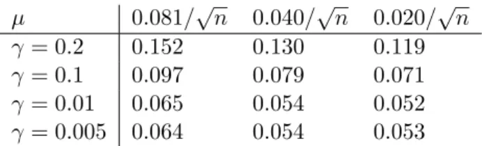
The output "res" is a list of twelve RKHS meta models. These meta models are evaluated using a new dataset, and their prediction errors are displayed in Table 7.
The minimum prediction error is associated with the pair (0.020/√n,0.01), and the
"best" RKHS meta model is then ˆf(0.020/√
n,0.01).
The performances of this procedure for estimating the Sobol indices is evaluated using the relative error (RE) defined as follows: