Potential of Using High Resolution Bus GPS Data to Assess Traffic Speeds

(1)

Portland State University

PDXScholar

Civil and Environmental Engineering Master's

Project Reports

Civil and Environmental Engineering

6-13-2016

Potential of Using High Resolution Bus GPS Data to Assess Traffic

Speeds

Nicholas B. Stoll

Portland State University, [email protected]

Let us know how access to this document benefits you.

Follow this and additional works at:

https://pdxscholar.library.pdx.edu/cengin_gradprojects

Part of the

Civil and Environmental Engineering Commons

This Project is brought to you for free and open access. It has been accepted for inclusion in Civil and Environmental Engineering Master's Project Reports by an authorized administrator of PDXScholar. For more information, please [email protected].

Recommended Citation

Stoll, Nicholas B., "Potential of Using High Resolution Bus GPS Data to Assess Traffic Speeds" (2016).Civil and Environmental Engineering Master's Project Reports. 26.

(2)

Potential of Using High Resolution Bus GPS Data to Assess Traffic Speeds

BY

Nicholas B. Stoll

A research project report submitted in partial fulfillment of the requirement for the degree of

MASTER OF SCIENCE IN

CIVIL AND ENVIRONMENTAL ENGINEERING

Project Advisor: Dr. Miguel Figliozzi

(3)

Acknowledgements

I would like to thank Steve Callas and Miles J. Crumley for graciously providing the data sets used in this analysis and for his support in understanding the intricacies of how the data is structured. I would also like to thank Dr. Miguel Figliozzi for his guidance and patience throughout this whole project. Lastly, I would like to thank my family for their unwavering support.

(4)

Abstract

This research investigates the potential of using archived high resolution bus data to describe traffic speeds on roadways; effectively using buses as probe vehicles. This is not only a simple and inexpensive way for transit agencies to better understand their road networks, but also utilizing buses as probe vehicles provides the potential to understand traffic conditions, to understand potential consequences of changes in road infrastructure, and many aspects of traffic utilizing already archived data. Using speed information derived from high resolution bus GPS data and stationary sensor data, this research examines the accuracy of bus GPS data and also discusses advantages, shortcomings, and limitations of utilizing GPS bus data to represent roadway speeds.

(5)

List of Tables

Table 1: Sample of 5-SR data set ... 5

Table 2: Final Regression Variables ... 8

Table 3: Regression Summary & Comparison ...10

Table 4: Regression Results, Eastbound 35th_{Sensor... 11}

Table 5: Regression Results, Westbound 24th_{Sensor ... 13}

Table 6: Regression Results, Westbound 35th_{Sensor ... 13}

Table 7: Regression Results, Eastbound 24th_{Sensor ... 14}

Table 8: Correlations, MAPE, and MPE for Original and New Locations... 19

Table 9: Bus Stop Locations Used in Regressions ... 19

Table 10: Summary Statistics ... 19

(7)

List of Figures

Figure 1: 24th_{location. WAV sensor and bus stops ... 4}

Figure 2: 35th_{location. WAV sensor and bus stops ... 4}

Figure 3: Before (grey) and after (black) bus points (24th WAV sensor) ...7

Figure 4: Before (grey) and after (black) bus points (35th WAV sensor) ...7

Figure 5: General case schematic... 8

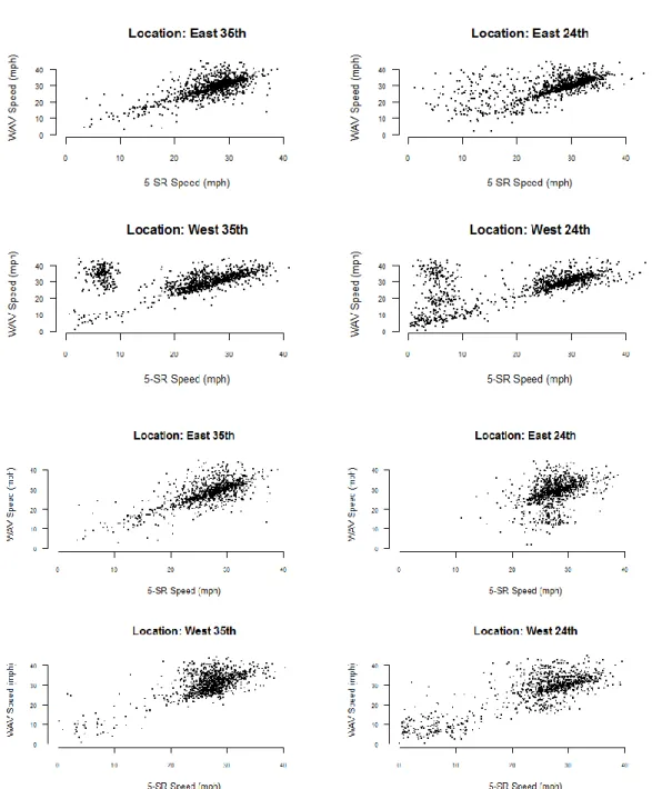
Figure 6: Original location speed comparison (top), updated location speed comparison (bottom). ... 15

Figure 7: 5-SR Speed vs. Sensor Speed (four locations) ... 16

Figure 8: Speed Profiles of Sensor and Original 5-SR Data ... 18

Figure 9: Bus stop information for eastbound buses ... 21

Figure 10: Percentage of Buses Stopping by Location and Direction ... 22

Figure 11: Westbound bus stop information... 23

Figure 12: Kernal Density Plots. ... 24

Figure 13: Speed plot, delay profile, and new location for analysis for East 24th_{... 25}

Figure 14: Speed plot, delay profile, and new location for analysis for West 24th_{... 26}

Figure 15: Speed plot, delay profile, and new location for analysis for East 35th_{... 27}

Figure 16: Speed plot, delay profile, and new location for analysis for West 35th_{... 28}

Figure 17: Aggregate speeds by location ... 29

Figure 18: Speeds calculated for 5-SR data by time of day ... 30

Figure 19: Speeds report for 10-second WAV increments ... 31

(8)

1

Introduction

Using data collected from buses and stationary sensors in Portland, Oregon, this study examines arterial traffic performance – building upon prior research – by using stationary sensors to examine the potential of high resolution bus data to examine traffic speeds.

Examining this potential is useful for understanding various applications of archived bus data, and for investigating the ability of high resolution bus data to reflect true traffic speeds. The potential flexibility offered by this use of archived data would allow public agencies to examine traffic conditions on roadways, without the need to install additional apparatus necessary to collect information. Mass transit agencies like Portland, Oregon’s Tri-County Metropolitan Transportation District (TriMet) have growing access and ability to analyze diverse sets of mass transit related data, and it is important to learn how these data can be used to manage and improve operations.

Background

Using buses as probe vehicles has been studied in the past (1), but with recent improvements in technology, systems that monitor both bus performance and location are becoming increasingly robust, less expensive, and easier to manage. With specific relation to TriMet, buses have already been used as probe vehicles to assess arterial performance and transit performance (2)(3). However, these studies were limited, only utilizing first generation stop level Active Vehicle Location (AVL) data to examine bus arrivals, pass bys, and bus stop departures. It was difficult to study space between bus stop data, and in order to estimate trajectories, proxies and estimates were used by researchers. In more recent years, and with the recent availability of high-resolution bus time and position information, bus travel speeds between stops and signal/queuing delays have been analyzed (4). The introduction of higher resolution data has removed much of the guesswork involved in understanding bus performance in-between bus stops, and added additional merit to the application of using buses as probes to assess traffic performance.

As a result of both the importance and myriad of data available, the study area, SE Powell Boulevard, has been examined in-depth. SE Powell Blvd. is a major arterial running east/west that connects downtown Portland, OR with Gresham, seeing an ADT of 35,000 to 45,000 vehicles per day. The performance of the adaptive traffic signal system (SCATS)(5), the impact of transit signal priority (TSP) on transit performance (6), air quality at bus stops (7), sidewalks at intersections (8), and sidewalks at mid-block locations (9) have all previously been examined within the confines of the study area. In addition, high resolution bus data have been

(9)

2

used to identify congestion and visualize bus speeds along the corridor (10). To add to this existing body of knowledge on arterial corridors, this research assesses the ability and

accountability of bus GPS data to understand traffic speeds. Through various comparisons of bus data with stationary traffic sensor data, which have been shown, and used extensively, to accurately characterize traffic (11), this research helps build upon previous research that validates high resolution bus data as a source for understanding traffic conditions.

Stationary sensor technologies have long been used as a reliable source of gathering information on roads and traffic conditions. While there is a wide variety of technologies employed by stationary sensors to measure conditions, those available to the researcher included radar sensors produced by Wavetronix. A full analysis of various radar technologies and their abilities to accurately detect traffic speeds and volumes can be found in a thesis written by Hemin Mohammed (11), or in an evaluation of traffic detection technologies written by Erik Minge in 2010 for the Minnesota Department of Transportation (12). Wavetronix DWR (Digital Wave Radar), the sensors used in this research, were one of the technologies analyzed in these two documents. It was found that this technology is very accurate for speed measurements (within 1.2 percent error for speed detection) (11), is very accurate in providing traffic volumes

(13), for reporting vehicle lengths (12), and is accurate under various weather conditions. With regards to reported speeds, WAV sensors (for here on out, this acronym will be used to refer to the sensors used in research) have been found to be accurate to within one mile per hour for free-flow traffic. On the whole, stationary sensors, especially Wavetronix radar sensors, are considered to be highly accurate devices used to measures roadway speeds. It was for this reason that these sensors were used as a baseline for comparisons with high resolution bus data.

Study Area

Along SE Powell Blvd., two WAV sensors are located at mid-block locations near cross-sections with 24th_{Avenue and 35}th_Avenue₍₁₅₎_{. The locations of these WAV sensors were}

chosen to best capture free flow traffic during peak hours, and are thus set back from major intersections (8). At the 24th _{WAV sensor location, SE Powell Blvd. is setup us as a two lane west}

and two lane east road, with a middle turn lane. For eastbound traffic, there is a dedicated right shoulder bus lane (which turns into a right turn lane on the approach to SE 26th_{Ave). At the 35}th

WAV sensor location, SE Powell Blvd. is two lanes each direction, with a left turn lane for

westbound traffic. While the location of the sensors is good for measuring peak traffic flow, their location is in close proximity to nearby bus stops, resulting in unique challenges for comparing bus GPS data with sensor data. The two WAV sensor locations, nearby bus stop locations, and

(10)

3

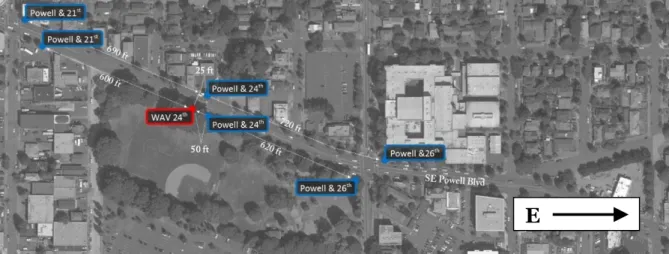
distances between the WAV sensors and the bus stops (in feet) are included in Figure 1 & Figure 2 and have the following characteristics:

 Eastbound 24th_{: The WAV sensor is roughly 50 feet upstream of the 24}th_{& SE Powell}

Blvd. bus stop (ID 4625) and over 600 feet downstream of the 21st_{& SE Powell Blvd. bus}

stop (ID 4622). It is also within close proximity of a crosswalk. The 24th_{and SE Powell}

Blvd. bus stop is not a very popular bus stop. On average, buses stop less than 20% of the time for most of the day, with spikes is stops during afternoon hours. Conversely, the stop at 21st_{and SE Powell Blvd. is very popular, averaging over 80% of buses stopping}

throughout the day (Figure 9, Figure 10) 1_.

 Eastbound 35th_{: This provided a great base case scenario because there were no bus}

stops within close proximity to the sensor, allowing for bus to potentially be operating within free flow traffic. The closest upstream bus stop is SE Powell Blvd. & 34th_(ID

4647), and is more than 350 feet away. Information regarding buses that stopped versus passed by this bus stop can be viewed in Figure 9 or Figure 10.

 Westbound 24th_{: There is a bus stop roughly 25 feet upstream of the sensor (SE Powell}

Blvd. & 24th_{, ID 4626), and the bus stop is within close proximity to a crosswalk. This bus}

stop is not very heavily trafficked, with a very low percentage of buses servicing the stop throughout the day. For most of the day, on average, buses stop roughly 25-35% percent of the time (Figure 10, Figure 11).

 Westbound 35th_{: Similar to the westbound 24}th_{, there is an upstream bus stop within}

close proximity to the sensor. SE Powell & 36th_{(ID 4649) is less than 200 feet upstream}

of the sensor. While not as frequently serviced as other bus at the various locations, this bus stop is serviced roughly 50% of the time. This fluctuates by time of day, with a higher percentage, and total number of buses, stopping during the morning hours (Figure 10, Figure 11).

The collection of these four movements and locations allowed for the analysis of three different scenarios: 1) no nearby bus stop, allowing for near free flow conditions (eastbound 35th_{); 2) a nearby upstream bus stop, where, if buses stopped, would provide a case where buses}

are accelerating into traffic as they pass the sensor (westbound 24th_{and 35}th_{); and 3) a nearby}

downstream bus stop, where, if buses stopped, would provide a case in which buses are

1_{A given Stop ID or bus stop name can be used to reference to these figures. These figures are located in} the Appendix.

(11)

4

decelerating as they pass the sensor (eastbound 24th_{). The analysis section of this paper is}

structured around particulars of these three scenarios.

Figure 1: 24th_{WAV location. WAV sensor (red) and bus stops (blue)}

Figure 2: 35th_{WAV location. WAV sensor (red) and bus stops (blue)}

Data

This section outlines and describes the various sources of data, the processes used to analyze the data, and the types of analyses used to examine the corresponding data sets.

TriMet Data

Data used from TriMet was supplied in the form of four different datasets: cyclic data, stop event data, stop data, and block data. Cyclic data, one of the more recent data effort from TriMet, was introduced in 2013 as a second generation AVL data set, and has finer granularity at 5-second intervals (referred to as 5-second, 5-SR data, or “breadcrumb” data) for time, position, and two unique bus identifiers (see Table 1 for dataset example). This is the high resolution data. The first identifier, trip number, is used to define a single bus trip (i.e. westbound from start to

E

(12)

5

finish of a route). The second identifier, stop number, is updated whenever the bus stops (i.e. scheduled bus stop or unscheduled stop). For example, in Table 1, all instances from the sample belong to the same bus trip, but the bus stopped three times, which is indicated when the stop number changes.

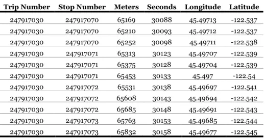
Table 1: Sample of 5-SR Dataset

Trip Number Stop Number Meters Seconds Longitude Latitude

247917030 247917070 65169 30088 45.49713 -122.537 247917030 247917070 65210 30093 45.49712 -122.537 247917030 247917070 65252 30098 45.49711 -122.538 247917030 247917071 65313 30123 45.49707 -122.539 247917030 247917071 65375 30128 45.49704 -122.539 247917030 247917071 65453 30133 45.497 -122.54 247917030 247917072 65531 30138 45.49697 -122.541 247917030 247917072 65608 30143 45.49694 -122.542 247917030 247917072 65685 30148 45.49691 -122.543 247917030 247917073 65763 30153 45.49685 -122.544 247917030 247917073 65832 30158 45.49677 -122.545

While the 5-SR data generally records time and location information every five seconds, it fails to do so when (1) the bus is stopped on the fifth second, i.e. wheels are not moving on the fifth or tenth second, (2) when the bus enters an administrator defined area, usually the bus stop itself. This is important for understanding minutely how 5-SR data operates around bus stops. The stop event and stop datasets contain information regarding instances where the bus stops. The stop data set contains information on type of stop— i.e. service stop, disturbance stop, pass through (bus doesn’t service a stop), and unplanned door open—as well as other general

information about how long the bus is stopped for. Stop event data, or first generation AVL, includes more in-depth information about the bus at the stop level. This includes dwell time, estimated bus load, ons, offs, and variety of other characteristics that judge a buses

performance. This first generation AVL data is what has been used in earlier research to explore using buses as probe vehicles (1)(2)(3). Stop event and stop data can be combined with the 5-SR data for a given trip number and stop number, but require the block data set to complete the merger. Merging the data sets allows for the examination of high resolution bus GPS data, which is telling us where the bus is, with bus stop level data, which is telling us what and how

(13)

6

WAV Sensor Data

The WAV sensors along SE Powell Blvd. record data in ten second increments, and include information, by lane, for the following items: occupancy, size of vehicle, and speed. Because WAV sensors record information by lane of traffic, only right lane information was used in the analysis. This is because buses are confined to the right lane at the analysis locations.

Processing the Data Sets

Comparing high resolution moving GPS data with stationary sensor data provided interesting challenges. With known GPS coordinates for the WAV sensors, the task involved finding one bus GPS coordinate on either side of the sensor, allowing for a speed between the two bus coordinate pairs which would best reflect the bus speed experienced during a given 10-sec sensor interval at the location of the sensor. First, the 5-SR bus data was divided into westbound and eastbound traffic. Next, a bearing and distance were calculated between each bus GPS point and a given WAV sensor—24th_{or 35}th_{. When this bearing changed drastically,}

threshold set at 170 degrees, the bus had past the WAV sensor, and the point information was recorded in a dataset (these points can be seen in Figure 3 and Figure 4). For example, if the bus was moving westbound with a bearing of -90 degrees, the bearing will remain relative constant for all GPS point prior to the sensor, until it passed the sensor, where, because the bearing is calculated between the GPS and the WAV sensor, would change to 90 degrees. This process was done for both westbound and eastbound traffic at both sensor locations. Using the timestamp for the before point, the closest ten second WAV increments were collected. Before point refers to the bus GPS point directly before a WAV sensor. Likewise, the after point refers to the GPS point directly after the sensor (these names will be used throughout the remainder of the paper). What resulted was a dataset of the closest, spatiotemporal, bus information for when an

individual bus was passing by each sensor. The final two datasets 1) 5-SR data containing bus information for the before and after points, and 2) WAV data containing stationary sensor information associated with each 5-SR point combination, were used to complete the remaining analysis. To understand what might have caused differences between the various high resolution bus data speed profiles and their associated sensor profiles, backwards linear regression models

(17) were run using independent variables of bus characteristics (i.e. did a bus stop at a given bus stop, estimated load of bus, or door open time) and general characteristics (i.e. distance from a bus point to the WAV sensor, sensor occupancy, sensor reported vehicle sizes, etc.), which were available from the two data sets.

(14)

7

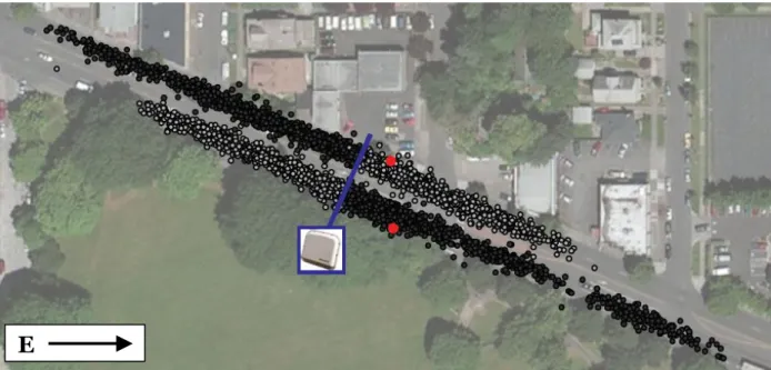
Figure 3: Before (grey) and after (black) bus points (24th WAV sensor). Bus stops indicated in red and WAV sensor indicated in blue.

Figure 4: Before (grey) and after (black) bus points (35th WAV sensor). Bus stop indicated in red and WAV sensor indicated in blue.

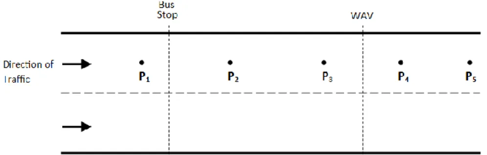
A theoretical case of data processing and of final variables used in regressions can explained using the Figure 5 schematic and variable definitions in Table 2. Direction of traffic is given for a two lane road, and points P1 through P5 represent consecutive bus GPS points of the

same bus trip number. The location of a bus stop and WAV sensor are provided as vertical dashed lines to easily show upstream and downstream GPS points. Bus stop information—from

E

(15)

8

the stop and stop event data sets—like estimated loads, ons, offs, and dwell time will be attached to each point following a given bus stop. So, points P2 through P5 will have associated bus stop

information from the theoretical bus stop. The before point is P3 and the after point is P4, as

they are the points that directly surround the WAV sensor.

Figure 5: General case schematic

Table 2: Final Regression Variables Dependent variable

The difference between WAV and 5-SR speeds. (WAV – 5-SR)

Independent variables

Variable Variable Description Type _SourceData

Distance: Sensor to Point

(before) Distance between WAV sensor and the before 5-SR breadcrumb Interval 5-SR Distance: Sensor to Point

(after) Distance between WAV sensor and the after 5-SR breadcrumb Interval 5-SR Sensor Speed WAV recorded speed for a given 10 second

interval Interval WAV

Dummy Variables

Variable Variable Description Type _SourceData

Bus Door Opened (before) Whether or not the doors were opened for the bus stop data associated with the before point.

(0=closed,1=open) Dummy Stop Event

Bus Door Opened (after) Whether or not the doors were opened for the bus stop data associated with the after point.

(0=closed,1=open) Dummy Stop Event

With regards to regression variables (Table 2), the variable “Distance: Sensor to Point (after)” refers to the distance between P4 and the WAV sensor. Similarly, “Distance: Sensor to

Point (before)” refers to the distance between P3 to the WAV sensor. The variables “Bus Door

Opened (before)” and “Bus Door Opened (after)” refer to whether, for the before or after point, the bus stop data associated with a point indicated the bus serviced the bus stop. For example, in

(16)

9

the schematic, if a bus stopped at the bus stop, both before and after variables would be 1. This is because there is no bus stop between the before and after points, and the bus stop data

associated with the before point will be the same as the after point. The remaining independent regression variable used, “Sensor Speed,” refers to the speed recorded by the WAV sensor over the 10 second interval associated with each bus trip number. The dependent variable used was the difference between the reported WAV speed and calculated bus speed (WAV speed – 5-SR speed).

Analysis

Several types of analyses were completed to compare speeds between the high resolution data and the stationary sensors. The first involved comparing aggregated speeds, over various timeframes, to examine the averaged speed profiles of the two data sources (Figure 8).

Correlations between these speed profiles were also calculated, and are displayed in Table 8. To more closely examine where and why the two speed profiles differed, plots comparing individual instances were created and regressions were run (Figure 6, Figure 7). Summary tables of the regressions are included (Table 10, Table 11), and individual case regressions on a location by location basis (Table 4, Table 5, Table 6, Table 7). For the regressions, data was subset to where the WAV sensor reported a speed greater than zero, the difference between the WAV speed and 5-SR speed was less than 40 mph, and the reported WAV speed was less than 45 mph2_{. A}

summary of the data included in the regression can be found in Table 9. The final piece of analysis included shifting the location of comparison between the high resolution bus data and the WAV sensors, meaning no more pair of GPS points directly surrounding a sensor (Figure 13, Figure 14, Figure 15, Figure 16). These new locations were chosen based on speed plots created specifically to view the high resolution data (10). Because many locations involved comparisons between buses that were either slowing down or speeding up, slightly shifting where high resolution data was gathered could remove this conflict, better match bus speeds with traffic speeds, and shift comparisons to a location where buses where experiences less delay. The process of selecting and processing the high resolution data did not change, just the location of where the bus data was collected. The same WAV 10-second increments as used in the

aforementioned analysis were again used for this second round of comparisons. Plots of speed data—WAV sensors, original 5-SR speeds, new location 5-SR speeds—by time of day help

2_{These subsets are for the following reasons: 1) the reported speed for Powell Blvd. is 35 mph, 2) if a bus} is stopped, and other vehicles are moving at free flow speed, the largest difference in speed should be less than 40 mph, and 3) there would be no vehicles present in the instances where the WAV sensor reports 0 mph.

(17)

10

visualize where fluctuations in speeds occurred and how the speed profiles changed with the new locations (Figure 17, Figure 18, Figure 19, Figure 20). The remainder of the section

describes these various forms of analysis according to the three scenarios outlined earlier: near free flow bus speeds, a nearby bus stop upstream from the sensor, and a bus stop slightly downstream from a sensor.

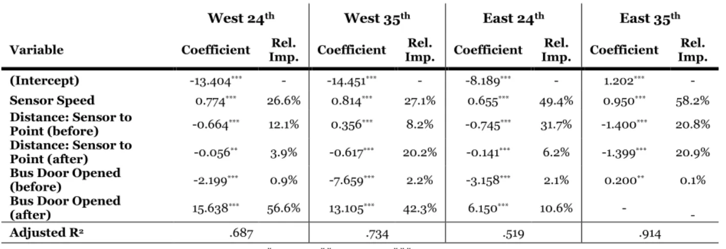
Table 3: Regression Summary & Comparison

West 24th _{West 35}th _{East 24}th _{East 35}th

Variable Coefficient _Imp.Rel. Coefficient _Imp.Rel. Coefficient _Imp.Rel. Coefficient _Imp.Rel.

(Intercept) -13.404*** _- _-14.451*** _- _-8.189*** _- _1.202*** _- Sensor Speed 0.774*** _26.6% _0.814*** _27.1% _0.655*** _49.4% _0.950*** _58.2% Distance: Sensor to Point (before) -0.664*** 12.1% 0.356*** 8.2% -0.745*** 31.7% -1.400*** 20.8% Distance: Sensor to Point (after) -0.056** 3.9% -0.617*** 20.2% -0.141*** 6.2% -1.399*** 20.9% Bus Door Opened

(before) -2.199*** 0.9% -7.659*** 2.2% -3.158*** 2.1% 0.200** 0.1% Bus Door Opened

(after) 15.638*** 56.6% 13.105*** 42.3% 6.150*** 10.6% - -

Adjusted R2 _.687 _.734 _.519 _.914

*p<0.1; ** p<0.05; ***p<0.01

Scenario 1: Near Free Flow Speeds

Eastbound buses around the 35th_{sensor can reach near free flow speeds because there}

are no bus stops in close proximity to the sensor, as the nearest one is a few hundred feet away. As a result, this location provides the most accurate speed comparisons between bus data and sensor data. At every aggregation level, sensor speeds and bus speeds were the most correlated, reaching in excess of 90% when aggregated by hour, with an overall MAPE of just 12% (Table 8). This is visually displayed in Figure 8, where bus speeds are consistently slightly slower than WAV sensor speeds, and in Figure 20, where trends lines between the two data sets exhibit similar patterns. At all speeds, speeds calculated from bus data match those reported by the sensor (Figure 6), with even the speed profiles matching in frequency and magnitude of reported speeds (Figure 12). The fluctuations in speeds caused by time of day—lower in the afternoon for eastbound travel—are seen in both the WAV speeds and 5-SR speeds, and at similar times (Figure 18, Figure 19). Because the location of comparison between the sensor and bus speeds already exists in a place with no associated delay (Figure 15), no new location was chosen for a second round of speed comparisons. Figure 15 also shows that the location of the sensor sits nicely between the two nearest bus stops, with no slow speeds associated with the stops being recorded by the sensor, and only mild congestion experienced during the pm peak. The backward linear regression results indicate the speed recorded by the sensor to be the most

(18)

11

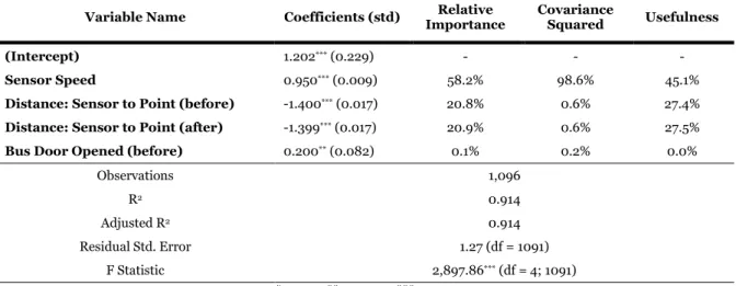
important variable in determining the difference between the WAV sensor and the calculated bus speed, and showed that as the sensor speed increased, the difference between the two speed profiles marginally increased (relative importance of 58%, Table 4). The distance of the before and after points from the WAV sensor were also found to be important, and as the distance increased, the difference between the two speed profiles decreased. The adjusted R2_{value for}

this scenario was .914.

Table 4: Regression Results, Eastbound 35th_Sensor

Variable Name Coefficients (std) _ImportanceRelative Covariance _Squared Usefulness

(Intercept) 1.202***_(0.229) _- _- _-

Sensor Speed 0.950***_(0.009) _58.2% _98.6% _45.1%

Distance: Sensor to Point (before) -1.400***_(0.017) _20.8% _0.6% _27.4%

Distance: Sensor to Point (after) -1.399***_(0.017) _20.9% _0.6% _27.5%

Bus Door Opened (before) 0.200**_(0.082) _0.1% _0.2% _0.0%

Observations 1,096 R2 _0.914 Adjusted R2 _0.914 Residual Std. Error 1.27 (df = 1091) F Statistic 2,897.86***_{(df = 4; 1091)} *p<0.1; ** p<0.05; ***p<0.01

Scenario 2: Nearby Upstream Bus Stop

This scenario applied to the two westbound locations, westbound 24th_{and westbound}

35th_{, where both locations exhibit a nearby upstream bus stop. While there was a very strong}

linear relationship between the WAV sensor and 5-SR bus information for the eastbound 24th

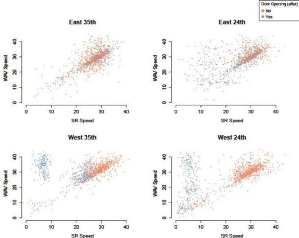
case, the relationship between the 5-SR data and the WAV sensor for these two locations is skewed by the presence of the nearby bus stops. From Figure 6, which plots WAV sensor speeds along the y-axis and 5-SR speeds along the x-axis, there are two distinct clusters of data points that appear. One cluster can be defined by low bus speeds but high sensor speeds, and the other cluster can be characterized by similar WAV and 5-SR speeds. When this same data is plotted again, but color is used to represent whether or not the bus serviced the upstream bus stop, the cluster of high WAV speeds but low 5-SR is almost completely accounted for (Figure 7). The schism is caused by buses servicing the upstream bus stops (seen as blue in Figure 6: Original location speed comparison (top four), updated location speed comparison (bottom four).Figure 7). This distinction is more clear for the westbound 24th_{case, while in the westbound 35}th_case,

some speeds between the WAV sensor and 5-SR data are very close even the bus serviced the stop. This is likely because there was enough time—this bus stop is further away the WAV sensor

(19)

12

then in the westbound 24th_{case—for the bus to have reached higher speeds as they pass the}

sensor. Figure 18 clearly shows the buses that are servicing the nearby bus stop, where they are seen as a band of low bus speeds which irrespective to time of day. Whereas the WAV speeds show fluctuations in speed, exhibiting higher levels of slow speeds in the morning, low bus speeds are seemingly independent of time of day. Looking at the density plots, both the

westbound 24th_{and westbound 35}th_{locations exhibits humps, or higher concentrations, of low}

speeds as compared to the WAV sensor (Figure 12). Again, these are the buses servicing the stop. The curve of higher speeds for bus data is also lower than speeds recorded by the sensor. As a result of these slower calculated bus speeds, the correlations between the bus speed data and sensor speed data are much lower than the case of free flow traffic (.79 at westbound 35th_and

.84 at westbound 24th_{for the 60-minute aggregate, Table 8). The regressions for these two}

locations confirm the importance of whether or not a bus serviced the upstream bus stop to determine the ability of the bus data to match the sensor data. The relative importance of this variable is by far the highest, 57% for westbound 24th_{and 42% for westbound 35}th_{, and was}

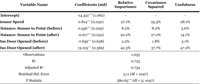
significant for both cases. While the magnitude of the sensor speed is still important for determining the difference between the sensor speed the calculated bus speed, it is not as important is in the free flow scenario. Adjusted R2_{values are .687 for the westbound 24}th

location and .734 for the westbound 35th_{location (Table 5, Table 6).}

In determining new locations to perform additional comparisons, Figure 14 & Figure 16 were used to find nearby locations were buses experienced minimal delay. For westbound 24th_,

this was roughly 215 feet downstream from the sensor. For westbound 35th_{, this was roughly 200}

feet downstream from the sensor. These two new locations are far enough away from a bus stop to ensure the buses are traveling near free flow, and as a result, are in locations of minimal bus delay. These new locations greatly improved the comparisons between the bus data and sensor data. There no longer existed a concentration of low speeds in the density plots. Instead, there was a more pronounced concentration of higher speeds (Figure 12). The speed plots no longer exhibited two distinct clusters, and instead appeared to have a linear relationship, much like the eastbound 35th_{free flow case (Figure 6). The new location bus data also exhibited speed}

fluctuations that better matched the WAV readings, with higher amounts of slow speeds in the morning instead of at all hours of the day (Figure 18, Figure 19). Lastly, the correlations between WAV speeds and 5-SR speeds increase from .76 to .92 for westbound 35th_{, and from .74 to .93}

for westbound 24th_{(at the 30-minute level), and both saw great decreases in MAPE (Table 8). By}

changing the location of the comparison to a nearby area where buses are experiencing minimal delay, the match between sensor speeds and calculated bus speed greatly improved.

(20)

13

Table 5: Regression Results, Westbound 24th_Sensor

(Intercept) -13.404***_(0.896) _- _- _-

Sensor Speed 0.774***_(0.027) _26.6% _14.9% _35.6%

Distance: Sensor to Point (after) -0.056**_(0.028) _3.9% _4.8% _0.2%

Bus Door Opened (before) -2.199***_(0.459) _0.9% _0.8% _1.0%

Bus Door Opened (after) 15.638***_(0.463) _56.6% _68.8% _49.5%

Observations 937 R2 _0.689 Adjusted R2 _0.687 Residual Std. Error 5.71 (df = 931) F Statistic 412.31***_{(df = 5; 931)} *p<0.1; ** p<0.05; ***p<0.01

Table 6: Regression Results, Westbound 35th_Sensor

(Intercept) -14.451***_(1.082) _- _- _-

Sensor Speed 0.814***_(0.030) _27.1% _25.3% _28.1%

Distance: Sensor to Point (before) 0.356***_(0.029) _8.2% _8.0% _5.6%

Observations 1,053 R2 _0.735 Adjusted R2 _0.734 Residual Std. Error 5.11 (df = 1047) F Statistic 580.63***_{(df = 5; 1047)} *p<0.1; ** p<0.05; ***p<0.01

Scenario 3: Nearby Downstream Bus Stop

For the eastbound 24th_{case, the nearest bus stop is slightly downstream from the sensor.}

As a result, buses that service the stop will have decelerated as they pass the sensor. However, this nearby downstream bus stop, SE Powell & 24th_{, is not very popular. This is likely why the}

two speed profiles are so highly correlated, reaching .94 when aggregated hourly, only second to the scenario where the buses operate in free flow speeds (Table 8). The speed plots reveal the speed calculated from bus data still undershoot the sensor speeds, but the comparison is much closer than the westbound cases (Figure 6, Figure 17). Similarly, the density plots revealed how

(21)

14

closely the speeds profiles matched (Figure 12). Interestingly, there was a concentration of low speeds for the WAV sensor. The speed plots by time of day are also very similar, with

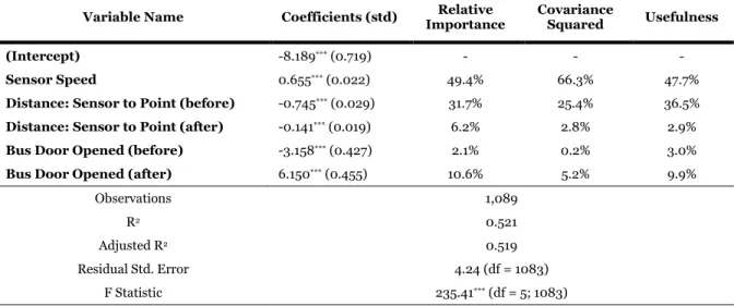
concentrations of lows speeds at all hours of the day, seen by both the sensor and the calculated bus speeds (Figure 18, Figure 19). Similar to the free flow scenario, sensor speed is the most important variable for regression results. However, the adjusted R2_{is the lowest of all cases, at}

just .519 (Table 7). The low use of the upstream bus stop means many buses are passing by at higher speeds, which likely accounts for the very similar speed profiles between the bus data and the sensor data, but does not account for the low adjusted R2_value.

While the WAV sensor is already located in an area of very low bus delay, just being outside the reach of the Powell Blvd. and 24th_{bus stop, a new location was chosen roughly 210}

feet upstream from the sensor (Figure 13). This location is halfway between two bus stops, and at a location that sees slightly less delay than the original location. Unlike the westbound cases, this new location has a large adverse effect on speed comparisons. Correlations between the two data sources decreased significantly (Table 8), speed distributions no longer matched well (Figure 12), the speed plot had two distinct clusters (Figure 6), and time of day fluctuations were dissimilar between the two data sources (Figure 18, Figure 19). Moving locations upstream took away many of the lower speeds found in the originally calculated bus data, which were also present in the WAV data, and resulted a much larger portion of high speeds. This can be seen in all plots of speed: the density plots, the time of day plots, and the direct speed comparison plots. Interestingly, while the trend line of the new location speed data is closer to that of the WAV speed data trend line, the shape no longer matches (Figure 20). This is different than what was seen in the westbound cases.

Table 7: Regression Results, Eastbound 24th_Sensor

(Intercept) -8.189***_(0.719) _- _- _-

Sensor Speed 0.655***_(0.022) _49.4% _66.3% _47.7%

Observations 1,089 R2 _0.521 Adjusted R2 _0.519 Residual Std. Error 4.24 (df = 1083) F Statistic 235.41***_{(df = 5; 1083)} *p<0.1; ** p<0.05; ***p<0.01

(22)

15

Figure 6: Original location speed comparison (top four), updated location speed comparison (bottom four).

(23)

16

Figure 7: 5-SR Speed vs. Sensor Speed (four locations, blue is door opened orange is door did not open)

Discussion & Conclusions

This paper has shown that archived high resolution bus data can be used to describe traffic speeds. While buses operate under different circumstances than regular traffic, variables that contribute to these differences can be accounted for, and analysis can be adjusted prior to speed validation; allowing for the use of high resolution bus data to serve as accurate probe data in a variety of scenarios. This is of importance because these data are easily accessible, archived, and provide the opportunity for transit agencies to examine traffic conditions at any location where a bus operates. While the bus speed data more closely matches sensor speeds when the buses operate in free flow conditions, slightly shifting the location of comparison has also been shown to provide accurate traffic speed comparisons. The important characteristics being the new location is nearby, buses at the original location exhibit delay, and the new location exhibits minimal bus delay. This research would benefit from a more in-depth examination of

differences between the two data sources, and to examine other scenarios where the relationship of the bus stops and sensors differ from what was available for this paper. This could include considering additional regression variables that may account for differences in speed profiles

(24)

17

(i.e. the presence of calculated acceleration or deceleration in bus data). Due to the way in which the bus system collects data, areas within close proximity to a bus stop raise critical issues when making comparisons between the dataset and stationary sensor: mainly with the way in which data is recorded and the delay experienced by the bus. This will vary depending on the data collection system, and it is important to have a keen understanding of how the system collects data. Understanding the conditions in which the buses operate is important before assessing the validity of the calculated speeds and their accuracy to actual traffic speeds.

(25)

18

Appendix

Figure 8: Speed Profiles of Sensor and Original 5-SR Data

(26)

19

Table 8: Correlations, MAPE, and MPE for Original and New Locations

Bin Sizes

Version location _min15 _min30 45 min _min60 MAPE _(%) MPE (%) Scenario

Original Locations

East 35th _0.92 _0.94 _0.96 _0.96 _12.16 _-3.65 _{Near free flow}

East 24th _0.80 _0.90 _0.90 _0.94 _17.94 _-6.96 Downstream bus

stop West 35th _0.60 _0.76 _0.68 _0.79 _24.11 _-11.87 _{Upstream bus stop} West 24th _0.70 _0.74 _0.70 _0.84 _45.50 _-29.94 _{Upstream bus stop} Updated Locations - - - - East 24th _0.53 _0.60 _0.62 _0.75 _21.81 _-9.33 _- West 35th _0.84 _0.92 _0.91 _0.94 _14.68 _-5.01 _- West 24th _0.83 _0.93 _0.92 _0.96 _26.30 _-12.98 _-

Table 9: Bus Stop Locations Used in Regressions

Data set

(# instances) Location ID Name Stop Before Point Point After East 24th ₄₆₂₂ ₂₁st ₁₀₈₉ ₆₈₉ (1089) 4625 24th _- ₄₀₀ East 35th ₄₆₄₇ ₃₄th ₁₀₉₆ ₁₀₉₆ (1096) West 24th ₄₆₂₆ ₂₄th ₂₉ ₇₆₂ (937) 4628 26th ₉₀₈ ₁₇₅ West 35th ₄₆₄₉ ₃₆th ₃₇₃ ₁₀₅₃ (1055) 4653 Cesar 682 2

Table 10: Summary Statistics

Independent Variables Location Min. 1st Qu. Median Mean 3rd Qu. Max. Std. Dev

Sensor Speed

west 24 2.40 26.00 30.00 28.60 33.50 45.00 7.69 west 35 3.00 27.50 31.10 30.76 34.60 44.10 5.82 east 24 1.60 25.80 29.40 28.49 32.70 44.40 6.60 east 35 2.80 25.40 28.80 28.33 31.90 44.60 6.01 Distance: Sensor to Point (before)

west 24 0.92 4.52 7.75 9.01 13.15 26.42 5.40

west 35 0.60 5.24 10.88 11.39 16.19 32.57 6.82

east 24 1.27 4.98 9.36 9.81 14.40 22.91 5.51

east 35 0.69 4.93 9.21 9.53 13.64 23.88 5.22

Distance: Sensor to Point (after)

west 24 0.62 5.71 11.56 12.40 17.06 34.44 7.85

west 35 0.72 5.06 9.38 9.82 13.95 28.05 5.47

east 24 0.77 4.70 8.13 12.82 18.40 42.11 10.66

east 35 1.17 5.00 8.92 9.49 13.64 24.20 5.22

Bus Door Opened (before)

west 24 0 1 1 0.77 1 1 0.42

west 35 0 1 1 0.93 1 1 0.26

east 24 0 1 1 0.82 1 1 0.38

east 35 0 0 0 0.33 1 1 0.47

Bus Door Opened (after)

west 24 0 0 0 0.35 1 1 0.48

west 35 0 0 0 0.48 1 1 0.50

east 24 0 0 1 0.52 1 1 0.50

(27)

20

Table 11: Regression Summary & Comparison

West 24th _{West 35}th _{East 24}th _{East 35}th

Variable Coefficient _Imp.Rel. Coefficient _Imp.Rel. Coefficient _Imp.Rel. Coefficient _Imp.Rel.

(Intercept) -13.404*** _- _-14.451*** _- _-8.189*** _- _1.202*** _- Sensor Speed 0.774*** _26.6% _0.814*** _27.1% _0.655*** _49.4% _0.950*** _58.2% Distance: Sensor to Point (before) -0.664*** 12.1% 0.356*** 8.2% -0.745*** 31.7% -1.400*** 20.8% Distance: Sensor to Point (after) -0.056** 3.9% -0.617*** 20.2% -0.141*** 6.2% -1.399*** 20.9% Bus Door Opened

(before) -2.199*** 0.9% -7.659*** 2.2% -3.158*** 2.1% 0.200** 0.1% Bus Door Opened

(after) 15.638*** 56.6% 13.105*** 42.3% 6.150*** 10.6% - -

Adjusted R2 _.687 _.734 _.519 _.914

(28)

21

Figure 9: Bus stop information for eastbound buses. Black indicates # of bus that serviced a stop, grey indicates # of bus that passed through. Listed by hour of the day.

(29)

22

(30)

23

Figure 11: Westbound bus stop information. Black indicates # of bus that services a stop, grey indicates # of bus that passed through. Listed by hour of the day.

(31)

24

Figure 12: Kernal Density Plots. Original location speed density plots (top), new location speed density plots (bottom)

(32)

25

(33)

26

(34)

27

(35)

28

(36)

29

Figure 17: Aggregate speeds by location for new bus location (bottom) versus original bus location (top)

(37)

30

Figure 18: Speeds calculated for 5-SR data by time of day. Original speeds (top), and new location speeds (bottom). Red trend line, and blue vertical lines at 7am, 11am, 4pm, and 8pm

(38)

31

Figure 19: Speeds report for 10-second WAV increments associated with bus trip numbers. Red trend lines, and blue vertical lines at 7am, 11am, 4pm, and 8pm.

Figure 20: Speeds aggregated in 30 minute bins by time of day. WAV sensor speeds(black), original 5-SR calculated speeds (red), and new location 5-SR calculated speeds (blue).

(39)

32

References

1. Hall, R., and N. Vyas. Buses as a Traffic Probe: Demonstration Project. Transportation Research

Record, Vol. 1731, No. 1, 2000, pp. 96–103.

2. Bertini, R., and S. Tantiyanugulchai. Transit Buses as Traffic Probes: Use of Geolocation Data for Empirical Evaluation. Transportation Research Record: Journal of the Transportation Research

Board, Vol. 1870, Jan. 2004, pp. 35–45.

3. Bertini, R., and A. El-Geneidy. Generating Transit Performance Measures with Archived Data.

Transportation Research Record: Journal of the Transportation Research Board, Vol. 1841, Jan.

2003, pp. 109–119.

4. Glick, T. B., W. Feng, R. L. Bertini, and M. A. Figliozzi. Exploring Applications of Second Generation Archived Transit Data for Estimating Performance Measures and Arterial Travel Speeds. Transportation Research Board, 2014.

5. Slavin, C., W. Feng, M. Figliozzi, and P. Koonce. A Statistical Study of the Impacts of SCATS Adaptive Traffic Signal Control on Traffic and Transit Performance. Annual Meeting of the

Transportation Research Board, Vol. 2250, No. June, 2012.

6. Albright, E., and M. Figliozzi. Factors Influencing Effectiveness of Transit Signal Priority and Late-Bus Recovery at Signalized-Intersection Level. Transportation Research Record: Journal of the

Transportation Research Board, Vol. 2311, Dec. 2012, pp. 186–194.

7. Moore, A., M. Figliozzi, and C. Monsere. Air Quality at Bus Stops. Transportation Research

Record: Journal of the Transportation Research Board, Vol. 2270, Oct. 2012, pp. 76–86.

8. Slavin, C., and M. Figliozzi. A Multimodal Evaluation of a Corridor Traffic Signal Performance : a case study on Powell Boulevard ( Portland , Oregon ). No. 2, 2009, pp. 1–12.

9. Moore, A., M. Figliozzi, and A. Bigazzi. Modeling the Impact of Traffic Conditions on the Variability of Mid-block Roadside Fine Particulate Matter Concentrations on an Urban Arterial.

Transportation Research Record, No. 2428, 2014, pp. 35–43.

10. Stoll, N., T. B. Glick, and Figliozzi. Utilizing High Resolution Bus GPS Data to Visualize and Identify Congestion Hot-spots in Urban Arterials. Transportation Research Record (pending), 2015. 11. Mohammad, Hemin J.; Schrock, Steven D.; Fitzsimmons, E. J. Accuracy of Traffic Speed and

Volume Data Detected Using Radar Technology. Transportation Research Record, 2015.

12. Minge, E., J. Kotzenmacher, and S. Peterson. Evaluation of Non-Intrusive Technologies for Traffic

Detection. St. Paul, 2010.

13. Mohammed, H. J. Evaluating the Accuracy of Speed and Volume Data Obtained via Traffic

Detection and Monitoring Devices. University of Kansas, 2015.

14. Keali’i, D. Evaluation of the Accuracy of Traffic Volume Counts Collected by Microwave Sensors. Brigham Young Univesity, 2015.

15. Bigazzi, A., W. Feng, A. Moore, and M. Figliozzi. Integrating Fixed and Mobile Arterial Roadway Data Sources for Transportation Analysis. 1–28.

(40)