On temporal-constrained sub-trajectory cluster analysis

On Temporal-Constrained Sub-Trajectory Cluster Analysis

Nikos Pelekis

_·

_{Panagiotis Tampakis}

_·

_{Marios Vodas}

_·

_{Christos Doulkeridis}

_·

_Yannis

Theodoridis

Abstract Cluster analysis over Moving Object Databases (MODs) is a challenging research topic that has attracted the attention of the mobility data mining community. In this paper, we study the temporal-constrained sub-trajectory cluster analysis problem, where the aim is to discover clusters of sub-trajectories given an ad-hoc, user-specified temporal constraint within the dataset’s lifetime. The problem is challenging because: (a) the time window is not known in advance, instead it is specified at query time, and (b) the MOD is continuously updated with new trajectories. Existing solutions first filter the trajectory database according to the temporal constraint, and then apply a clustering algorithm from scratch on the filtered data. However, this approach is extremely inefficient, when considering explorative data analysis where multiple clustering tasks need to be performed over different temporal subsets of the database, while the database is updated with new trajectories. To address this problem, we propose an incremental and scalable solution to the problem, which is built upon a novel indexing structure, called Representative Trajectory Tree (ReTraTree). ReTraTree acts as an effective spatio-temporal partitioning technique; partitions in ReTraTree correspond to groupings of sub-trajectories, which are incrementally maintained and assigned to representative (sub-)trajectories. Due to the proposed organization of sub-trajectories, the problem under study can be efficiently solved as simply as executing a query operator on ReTraTree, while insertion of new trajectories is supported. Our extensive experimental study performed on real and synthetic datasets shows that our approach outperforms a state-of-the-art in-DBMS solution supported by PostgreSQL by orders of magnitude.

Keywords cluster analysis, temporal-constrained (sub-)trajectory clustering, moving objects, indexing

† _{Nikos Pelekis}

Dept. of Statistics & Insurance Science, University of Piraeus, Piraeus, Greece E-mail: npelekis@unipi.gr

Panagiotis Tampakis Marios Vodas Yannis Theodoridis Dept. of Informatics, University of Piraeus, Piraeus, Greece E-mail: {ptampak, mvodas, ytheod}@unipi.gr

Christos Doulkeridis

Dept. of Digital Systems, University of Piraeus, Piraeus, Greece E-mail: cdoulk@unipi.gr

1.

Introduction

Nowadays, huge volumes of location data are available due to the rapid growth of positioning devices (GPS-enabled smartphones, on-board navigation systems in vehicles, vessels and planes, smart chips for animals, etc.). This explosion of data already contributes in what is called the Big Data era, raising new challenges for the mobility data management and exploration field (Giannotti et al. 2011; Pelekis and Theodoridis 2014). Efficient and scalable trajectory cluster analysis is one of these challenges (Zheng 2015; Yuan et al. 2016). The research so far has focused on adapting well-known solutions that are effective for legacy data types to trajectory datasets. Thus, a typical approach is to transform trajectories to multi-dimensional (usually, point) data, in order for well-known clustering algorithms to be applicable. For instance, CenTR-I-FCM (Pelekis et al. 2011) builds upon a Fuzzy C-Means variant. Another approach is to focus on effective and efficient trajectory similarity search, which is the basic building block of every clustering approach. Once one has defined an effective similarity metric, she can adapt well-known algorithms to tackle the problem. For instance, TOPTICS (Nanni and Pedreschi 2006) adapts OPTICS (Ankerst 1999) to enable whole-trajectory clustering (i.e. clustering the entire trajectories), and TRACLUS (Lee et al. 2007) exploits on DBSCAN (Ester et al. 1996) to support sub-trajectory clustering.

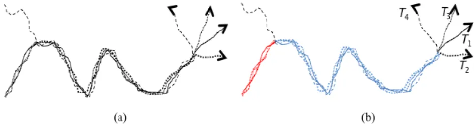
Sub-trajectory clustering is a typical cluster analysis problem in Moving Object Databases (MOD). Fig. 1 illustrates a working example, i.e. a dataset consisting of four trajectories, T1, …, T4 (please note that the time dimension has been ignored for visualization reasons). Upon this dataset, the goal of sub-trajectory cluster analysis is to identify two clusters (coloured red and blue, respectively) and five outliers (coloured black). The challenging issue is to depart from the (entire) trajectory grouping into clusters, by first identifying the best partitioning of each trajectory into sub-trajectories and then performing cluster analysis upon those entities. For instance, due to the deviation of the trajectories illustrated in Fig. 1(a) at the end of their lifespan, clustering the entire trajectories might probably result to either no cluster at all (with all four trajectories labelled as outliers) or a single cluster consisting of all four trajectories; with the result depending on the sensitivity of the underlying trajectory similarity function and auxiliary parameters of the clustering algorithm. On the other hand, working at the sub-trajectory level we will be able to identify the red and blue clusters of sub-trajectories as well as the black outliers (see Fig. 1(b)).

(a) (b)

Fig. 1 Four trajectories (a) before (b) after sub-trajectory clustering

Finding a solution to the above described sub-trajectory clustering problem is challenging; what is even more challenging, is how one can support incremental and progressive cluster analysis in the context of dynamic applications, where (i) new trajectories arrive at frequent rates, and (ii) the analysis is performed over different portions of the dataset, and this might be repeated several times per analysis task.

As motivational example, consider the Location-based Services (LBS) scenario where LBS users transmit their trajectories to a central LBS server, e.g. when their trip is completed. From the server side, a MOD system is responsible for organizing user traces, aiming to support extensive (usually incremental and explorative) querying and mining processes. Since users (the data producers) transmit their location information in batch mode and asynchronously, the underlying data management framework should be able to handle this kind of information transmission. In other words, as we are especially interested in cluster analysis, the data server should be able to cluster users’ trajectories in an incremental fashion. Clearly, the above techniques fail to meet such a specification.

Coming back to the example of Fig. 1, two main challenges need to be confronted: (i) given the addition of a new trajectory in the existing set of four trajectories, how can cluster analysis be performed over the updated data without applying the (quite expensive) clustering process from scratch, and (ii) how could we organize these trajectories so as to retrieve clusters valid in an ad-hoc temporal period of interest, without re-applying the clustering for the user-defined temporal period?

In this paper, we address the challenge of efficient and effective temporal-constrained sub-trajectory cluster analysis, by proposing an incremental and progressive solution to the problem. To this end, we propose a novel indexing scheme for large MODs, which is designed upon optimally selected samples of sub-trajectories, called Representative Trajectories, hence the term ReTraTree. Each sub-trajectory of this type acts as the representative of a group (cluster) of sub-trajectories. Thus, ReTraTree may be considered as a data structure

that organizes (sub-)trajectories in a hierarchical fashion, while having small, but in any case adaptable, memory footprint. Based on its design, ReTraTree is able to incrementally partition and cluster trajectories as they are inserted in the MOD. Interestingly, the actual clustering process for the user-defined temporal period of interest, called Query-based Trajectory Clustering (QuT-Clustering), is performed as simply as a query execution upon the ReTraTree.

The contributions of our work are summarized below:

• we introduce the temporal-constrained sub-trajectory cluster analysis problem, which is a key problem for supporting progressive clustering analysis;

• we design ReTraTree, an efficient indexing scheme for large dynamic MODs, which is based on

representative trajectories found in the dataset;

• as a solution to the problem of study, we devise QuT-Clustering, a sub-trajectory clustering algorithm

running as simply as a query operator upon ReTraTree;

• we facilitate incremental trajectory cluster analysis by exploiting the incremental maintenance of

ReTraTree along with the query-based clustering approach of QuT-Clustering;

• we perform an extensive experimental study upon real and synthetic datasets, which demonstrates that

our in-DBMS implementation outperforms a state-of-the-art PostgreSQL extension by several orders of magnitude

.

The rest of the paper is organized as follows: Section 2 formally defines the problem of temporally-constrained sub-trajectory cluster analysis. Section 3 presents the ReTraTree structure and its maintenance algorithms while Section 4 puts ReTraTree in action, in other words it provides the QuT-Clustering algorithm, also providing a complexity analysis of the entire framework. Section 5 presents our experimental study. Section 6 reviews related work. Section 7 concludes the paper and outlines future research directions.

2.

Problem Setting

In this section, we provide the necessary definitions and terminology. Table 1 summarizes the definitions of the symbols used in the paper.

Table 1: Symbol table

Symbols Definitions

D a dataset D = {T1, … , TN} of N trajectories

T a trajectory of D, whose length is |T| (in terms of number of points composing it)

xt.s (xt.e) starting (ending) timestamp of the time-varying object _{timestamp of trajectory T} x, e.g. Tt.s (Tt.e) is the minimum (maximum)

l lifespan of D, namely the temporal period [min(Tt.s), max(T’t.e)), ∀ T, T’∈D

pi i-th (3D) point of trajectory T, pi = (xi, yi, ti)

ei i-th (3D) line segment of T, ei = (pi, pi+1)

li lifespan of line segment ei, namely the temporal period [ti, ti+1)

S set of sub-trajectories partitioning trajectory T

Si i−th sub-trajectory of trajectory T

V(e, e’) voting function between two segments e and e’ belonging to trajectories T and T’, respectively

𝑉!!! voting descriptor of trajectory T with respect to T’

𝑉!! voting descriptor of trajectory T with respect to trajectory dataset D

𝑉!! voting of a trajectory dataset D with respect to T

𝑉!!! _{voting descriptor of trajectory dataset D with respect to trajectory dataset D’}

R Sample of representative sub-trajectories R ={R1,..., RM}

C clustering of sub-trajectories in M clusters, C = {𝐶!!,…,𝐶!!}, 𝐶!!∩𝐶!! = ∅, i ≠ j, with

sub-trajectory Ri representing cluster 𝐶!! of sub-trajectories

M cardinality of C (and R)

Out set of outlier sub-trajectories

W the user-defined time window (W ∈ l) for which we want to discover the sub-trajectory clusters

Definition 1 (Voting between segments of two trajectories): Given two segments e and e’ belonging to trajectories T and T’, respectively, the voting function V(e, e’) that calculates the voting e receives by e’ is given by Eq.(1):

𝑉 𝑒,𝑒′ =𝑒!  !

!_!,!!

!∙!! (2)

where the control parameter σ > 0 shows how fast the function (“voting influence”) decreases with distance.

Since Euclidean distance D(t) is symmetric, distance d(e, e’) is symmetric as well. As such, it holds that V(e, e’) = V(e’, e); it also holds that 0 ≤ V(e, e’) ≤ 1. If the two segments are almost identical, i.e. distance d(e, e’) is close to zero, the voting function gets value close to 1. On the other hand, high values of distance d(e, e’) result in voting close to zero.

We can generalize the above discussion to define the representativeness of a trajectory with respect to another trajectory. Notice that the definition that follows is applicable to trajectories as well (since a sub-trajectory is itself a sub-trajectory, essentially a set of consecutive segments).

Definition 2 (Voting descriptor and average voting of a trajectory with respect to another trajectory): Given a trajectory T of length |T| and another trajectory T’, the voting descriptor

𝑉

𝑉

of dimensionality |T|−1 where wildcard

′

∗

′

𝑉

𝑉

to trajectory T’.

Obviously, the voting descriptor is not symmetric, i.e.

𝑉

𝑉

Definition 3 (Voting descriptor of a trajectory with respect to a trajectory dataset): Given a trajectory dataset D and a trajectory T of cardinality |T|, T ∉ D, the voting descriptor

𝑉

vector 𝑉!!: 𝑉 𝑒!,∗ !!∈! ,…, 𝑉 𝑒!!!,∗ !!∈! (4) of dimensionality |T|−1 where wildcard

∗

d(ei, ·), i = 1, …, |T|−1.

Recall that (i) the vote a segment can receive by another segment is a value ranging from 0 to 1, according to Eq.(2), and (ii) only one segment from each trajectory votes for a given segment of another trajectory, i.e. its nearest. This implies that the total voting – the sum of votes – received by a given segment is a value ranging from 0 (if all members of D vote 0) to N (if all members of D vote 1). To exemplify the above, back to the example of Fig. 1, voting descriptor 𝑉_!!!!,!!,!! _{presents in general higher values than voting descriptor 𝑉}

!_!!!,!!,!!

since T1 is more centrally located than T4 in the dataset.

Definition 4 (Voting of a trajectory dataset with respect to a trajectory): Given a trajectory dataset D of cardinality N and a trajectory T of cardinality |T|, T ∉ D, voting

𝑉

𝑉!! = 𝑎𝑣𝑔 𝑉!!!   !!∈!

(5) that accumulates the average voting of all trajectories 𝑇′∈𝐷 with respect to

𝑇

Definition 5 (Voting of a trajectory dataset with respect to another trajectory dataset): Given a trajectory dataset D of cardinality N and another (reference) trajectory dataset D’ of cardinality N’, D ∩ D’ = ∅, voting 𝑉!!! of D with respect to D’ is a value calculated as follows:

𝑉_!!!_{= 𝑉}

!!

!∈!! (6)

Now we define the temporally-constrained sub-trajectory clustering problem that we address in this paper. Let W represent a time window within the lifespan of D, i.e. W ∈ l. Further, let DW denote the set of sub-trajectories partitioning the sub-trajectories in D, which are temporal-constrained within W. Formally:

Problem (Temporal-constrained sub-trajectory clustering): Given (i) a trajectory database D = {T1, …, TN} of lifespan l, consisting of N trajectories of moving objects, and (ii) a time window W (W ∈ l), the

temporal-constrained sub-trajectory clustering problem is to find: (a) a set C =

{𝐶

,

…

,

𝐶

}

sub-trajectories,

𝐶

𝐶

called representative sub-trajectories, and (b) a set Out of outlier sub-trajectories, Out ∈ DW, so that voting

𝑉_!!_{!!! of dataset D}

W−R with respect to R is maximized:

The above problem is quite challenging, for a number of reasons. First, the segmentation (or partitioning) of trajectories found in D in sub-trajectories cannot be predefined nor is the result of a third-party trajectory segmentation algorithm, such as (Buchin et al. 2010; Lee et al. 2007; Li et al. 2010b). Instead, it is problem-driven: it is the clustering algorithm that solves the above problem that is responsible to find the best segmentation of trajectories into sub-trajectories. Practically, it is the clustering algorithm that is responsible to detect the red and blue parts of trajectories in Fig. 1, given that the analyst requires a clustering providing as time window W the whole lifespan of the dataset. Second, the optimization of the above scenario is a hard problem, since the solution space is huge. Third, one has to define the technique for selecting the set of the most representative sub-trajectories, whose cardinality M is unknown. Fourth, as already discussed, in a real MOD setting, the solution should support incremental updates. Put differently, data updates should be accommodated as soon as they come and update the existing clusters at low cost, instead of performing a new clustering process from scratch. Finally and most importantly, since clustering is applied over different portions of the dataset, and this might be repeated several times per analysis task, the solution to the problem should be repeatable for all the different time windows W that are of interest during explorative analysis. This comprises a novel feature and a major contribution of our work, since existing solutions for sub-trajectory clustering are not able to support progressive clustering analysis taking into account temporal constraints as filters.

3.

The ReTraTree Indexing Scheme

We start this section with an overview of the ReTraTree indexing scheme (Section 3.1) and we continue with the algorithms that are necessary for its maintenance (Sections 3.2 – 3.4).

3.1 ReTraTree Overview

ReTraTree consists of four levels: the two upper levels operate on the temporal dimension while the 3rd _{level is} built upon the spatio-temporal characteristics of the trajectories. The idea is to hierarchically partition the time domain by first segmenting trajectories into sub-trajectories according to fixed equi-sized disjoint temporal periods, called chunks (1st _{level partitioning). Then, each chunk is organized into sub-chunks, which form a} partitioning of sub-trajectories within each chunk (2nd _{level partitioning). Notice that sub-chunks may overlap in} time, i.e. they are not temporally disjoint.

Example 1 Fig. 2 illustrates six trajectories, T1,…, T6 spanning in two days (called Day 1 and Day 2). The dataset is split into two chunks at day-level, with mauve (green) colored sub-trajectories corresponding to the evolution of moving objects on Day 1 (Day 2, respectively). Furthermore, the chunk corresponding to Day 1 is subdivided to two sub-chunks, corresponding to <T1, T2, T3, T4> and <T5, T6>, respectively. Although not illustrated in the figure, the first sub-chunk is valid during [20:00, 0:00) of Day 1 while the second sub-chunk is valid during [22:00, 0:00) of Day 1, thus they are overlapping in time. Especially for the first sub-chunk, we also illustrate the projection of the four trajectories on the spatial domain, which corresponds to Fig. 1(b).

Fig. 2 Six trajectories, spanning in 2 days, split into daily chunks

Next, the sub-trajectories of each sub-chunk are clustered on the spatio-temporal domain with a sampling-based algorithm. In the previous example, this step results in the formation of two clusters of sub-trajectories (in red and blue) and five outlier sub-trajectories (in black), see Fig. 1(b). Thus, ReTraTree maintains only the representatives at the 3rd level of the structure, while the actual clustered data are archived at the 4th level. Fig. 3 (and the paragraphs that follow) present ReTraTree in detail. Note that the top-three levels of the ReTraTree reside in main memory and only the 4th _{level is disk-resident.}

1st level (chunks). The root of the ReTraTree consists of p entries, p ≥ 1, corresponding to chunks sorted by time (in the example of Fig. 2, at daily level). Note that for each chunk Hi , i = 1, …, p, there is no need to maintain the actual temporal periods in the index nodes since they correspond to fixed equal-length splitting intervals. Each entry Hi maintains only a pointer to the respective set of sub-chunks Hi,n, n ≥ 1, under this chunk. The set of all chunks forms the 1st level of the structure.

y

x

2

2nd _{level (sub-chunks). For each chunk, there is a set of sub-chunks, actually a sequence of triples < H} i,n.per, Hi,n.R, Hi,n.Out >, n ≥ 1, where per is a temporal period [pert.s, pert.e) when the sub-chunk is valid (in the example of Fig. 2, [20:00, 0:00) and [22:00, 0:00), respectively for the two sub-chunks of Day 1), while R (Out) are pointers to the set of representative (outlier, respectively) sub-trajectories belonging to sub-chunk Hi,n. The sequence of triplets is ordered by <pert.s, pert.e>. The set of all sets of sub-chunks forms the 2nd level of the structure.

3rd level (cluster representatives). For each sub-chunk, the entries of set R consist of pairs <Rj, 𝐶!_!>, j ≥ 0,

where each entry includes the representative sub-trajectory Rj and a pointer 𝐶!! to the subset of sub-trajectories

belonging to that sub-chunk and forming a cluster around Rj. Note that j = 0 implies that there may exist sub-chunks with zero clusters (i.e. including outliers only). The set of all sets of cluster representatives (along with the pointers to actual data) forms the 3rd _{level of the structure.}

4th _{level (raw trajectory data and outliers). The sets of actual sub-trajectories that compose clusters 𝐶} !! are

stored at the 4th level of the structure. For each sub-chunk Hi,n, there corresponds a set Di,n consisting of triples <sub-trajectory-id, 𝐶_!!, sub-trajectory-3D-polyline> that keep the information about which sub-trajectory belongs to which cluster. On the other hand, set Out contains the outlier sub-trajectories of that sub-chunk. The outlier sub-trajectories are appropriately indexed in a 3D-R-tree structure (Theodoridis et al. 1996). The clustering process of sub-trajectories belonging to a sub-chunk, during which we detect sets S and Out, is a key process for ReTraTree and is described in detail in Section 5.

Fig. 3 Overview of the ReTraTree indexing scheme

How ReTraTree handles a new trajectory is discussed in the subsections that follow. 3.2 Hierarchical temporal partitioning

Given a trajectory database D of lifespan l (whose duration is denoted as |l|), a new trajectory T, and a fixed partitioning granularity p, applicable at the ReTraTree 1st _{level, T is partitioned into a number of sub-trajectories} Si, i ≥ 1, where the sub-trajectory Si is the restriction of T inside a temporal period pi,

𝑝!=

|𝑙|∙ 𝑖−1

𝑝 ,

|𝑙|∙𝑖

𝑝 ,1≤𝑖≤𝑝

where |𝑙| _𝑝 is the length of each time interval (i.e. the duration of the lifespan of each chunk) and timestamps

𝐷!.!+|𝑙|∗ 𝑖−1 𝑝,  2≤𝑖≤𝑝 are called splitting timestamps. As such, every trajectory in the dataset is partitioned into sub-trajectories using the same (pre-defined, according to granularity p) splitting timestamps. This chunking process is applied incrementally, whenever a batch of new recordings from a moving object arrives. In case of a new trajectory with temporal information that exceeds the last existing chunk, a new chunk is created and the set of chunks CK is extended.

At the 2nd _{level, each chunk is subdivided into (possibly, overlapping) sub-chunks. Specifically, a chunk is} split into sub-chunks by grouping the sub-trajectories contained in the chunk, according to the following definition. Out R Di,n 1st level chunks 2nd _level sub-chunks 3rd level cluster representatives 4th _level raw trajectory data H1 H2 … Hi … Hp Hi,1 Hi,2 …

• • • • • •

Definition 6 (Grouping of sub-trajectories in the same sub-chunk): Given a temporal tolerance parameter τ

and two sub-trajectories S ∊ T and S’∊ T’ belonging to the same chunk, these sub-trajectories can be grouped together in the same sub-chunk if their starting (ending) timepoints differ at most τ/2, respectively. Formally, it

should hold that:

𝑆!.!−𝑆′!.! ≤𝜏 ₂∧ 𝑆!.!−𝑆′!.! ≤𝜏 ₂ (8)

Note that the above definition is not deterministic as there might be a sub-trajectory S’’∊ T’’ that also satisfies this condition. We handle this case by grouping the sub-trajectories when this condition is satisfied for the first time. Thus, we do not define and we do not search for a kind of “best-matching” sub-chunk. The reasons for this choice is that we are in favor of a very efficient insertion process, while we do not care about an optimal matching as this issue will be handled when the analyst asks for a clustering analysis. Regarding tolerance parameter τ, it is a user-defined parameter and can be exploited to impose an either stricter or looser

notion of grouping. It also implies that e.g. when τ is set to 10 minutes, a sub-trajectory of less than 20 minutes duration cannot be grouped together with a sub-trajectory of more than 30 minutes duration.

3.3 Sampling-based sub-trajectory clustering

As already mentioned in Section 3, maximizing Eq. (7) is a hard problem. In order to tackle it we adopt a methodology for the optimal segmentation and selection of a sample of sub-trajectories from a trajectory dataset. Thus, in Fig. 4, we outline the Sampling-based Sub-Trajectory Clustering (S2T-Clustering) algorithm, a two-step process that relies on a sub-trajectory sampling method, proposed in (Panagiotakis et al. 2012). Briefly, S2_{T-Clustering relies on the output of the afore-mentioned sampling method (1}st _{step), which is a set of} sub-trajectories in the MOD that can be considered as representatives of the entire dataset. These samples serve as the seeds of the clusters, around which clusters are formed based on a greedy clustering algorithm (2nd step).

Algorithm S2_T-Clustering

Input: MOD D = {T1 , T2 , … , TN }, ε, δ

Output: Sampling set R, Clustering C, Outlier set Out. 1. (R, S) ß Sampling(D, ε)

2. (C, Out) ß GreedyClustering(R, S, δ) 3. return (R, C, Out)

Fig. 4S2_{T-Clustering for building ReTraTree sub-chunks}

The first step of S2_{T-Clustering algorithm (line 1) invokes the Sampling method, which aims to solve an} optimization problem, namely to maximize the number of sub-trajectories represented in a sampling set. In a few words, Sampling calculates the voting descriptor

𝑉

described in Def. 3. Then, based on this signal, each trajectory is partitioned into sub-trajectories having homogeneous representativeness (i.e. the representativeness of all segments in a sub-trajectory does not deviate over a user-defined threshold), irrespectively of their shape complexity. According to (Panagiotakis et al. 2012), a trajectory should have at least w points in order for the segmentation to take place. Thus, w is an application-based parameter of Sampling that acts as a lower bound of the length of a trajectory under segmentation. Subsequently, Sampling selects a sampling set R={R1,…,RM} of sub-trajectories, which are hereafter considered as the representatives of D. Note that the number M of sub-trajectories is not user-defined; instead, it is dynamically calculated by the method itself. This is achieved by tuning Sampling with a parameter ε (ε>0 and

εà0), the role of which is to terminate the internal iterative optimization process when the optimization formula is lower than a given threshold (i.e. the ε parameter). Back to the example of Fig. 1, the above voting-and-segmentation phase would result in segmenting trajectory T1 into three sub-trajectories (coloured red, blue, and black, respectively, in Fig. 1) according to its representativeness; similar for the rest trajectories of the MOD.) Then, Sampling would intuitively select two trajectories as representatives, one from the blue sub-trajectories, and one from the red sub-trajectories.

At its second step (line 2), S2T-Clustering uses sampling set R in order to cluster the sub-trajectories of the dataset according to the following idea: each sub-trajectory in the sampling set is considered to be a cluster representative. More specifically, clustering is performed by taking into account sampling set R = {R1,…,RM} and vector of votes (i.e. representativeness) 𝑉_!

! !_!

(actually we use the average voting 𝑎𝑣𝑔 𝑉_!

! !_!

) between sub-trajectories of the original MOD Si∈ D − R with respect to the representative sub-trajectories Rj∈ R. Recall that 𝑉_!

! !_!

(Def. 2) consists of |Si| elements, where each one represents the voting that the segments of Si receive from the segments of Rj. To this end, in order for the S2T-Clustering algorithm to maximize Eq. (7) for the special case where the time window W corresponds to the lifespan l of D, the cluster 𝐶_!! of a representative sub-trajectory of the sampling dataset Rj ∈ R, i.e. the set of sub-trajectories that are assigned to cluster 𝐶!_!, is

𝐶!_! = 𝑆!∈𝐷−𝑅:𝑎𝑣𝑔 𝑉!_! !_! ≥𝑎𝑣𝑔 𝑉_!!_!! _,∀𝑅 !∈𝑅∧𝑎𝑣𝑔 𝑉!_! !_! ≥𝛿 (9)

On the other hand, set Out of outliers consists of sub-trajectories that have been assigned to no cluster: 𝑂𝑢𝑡= 𝑆!∈𝐷−𝑅−𝐶!_!,∀𝑅!∈𝑅 (10) The algorithm outlined in Fig. 4 simply iterates through all the representative sub-trajectories Rj∈ R of the sampling dataset R and applies the constraints of Eq. (9). Parameter δ is a positive real number between 0 and 1 that acts as a lower bound threshold of similarity between sub-trajectories and representatives. As such, it controls the size of the clusters C and the outlier set Out.

3.4 ReTraTree maintenance

S2_{T-Clustering does not support arbitrary time windows nor dynamic data. The additional challenge that we} have to address is to efficiently support such a clustering for arbitrary time windows and dynamic data. To achieve this, we need to efficiently support insertions of new trajectories in the ReTraTree.

The incremental maintenance of the ReTraTree, whenever a batch of recordings of a moving object (i.e. a trajectory T) arrives, is supported by the ReTraTree-Insert algorithm outlined in Fig. 5. We have already described how our method incrementally performs the first phase of partitioning in the time dimension (line 1). The update_chunks function returns the set of chunks H and the respective set of sub-trajectories S that correspond to the input trajectory T, i.e. the sub-trajectories Si that intersect temporally with chunk Hi. Then, the algorithm assigns each sub-trajectory Si to an appropriate sub-chunk (lines 2-4). This is actually checked by the find_subchunk function which, instead of applying Def. 6 between Si and the other trajectories in the sub-chunk, simply tests whether the following inequality holds: |Si,t.s – Hi,n,t.s| ≤τ /2  ∧ |Si,t.e – Hi,n,t.e | ≤τ /2. To gain this efficiency, the implicit assumption is that the temporal borders of each sub-chunk are left unchanged since its initialization with its first sub-trajectory. If there is not a matching sub-chunk with respect to time (line 5), a new sub-chunk is created, which is initialized with an empty representative set R, and an outliers set Out including the unmatched sub-trajectory (line 17). If there is an appropriate sub-chunk for the sub-trajectory under processing (line 5), the algorithm tries to greedily assign it to the best existing cluster (lines 6-13). If this attempt fails (line 14), the algorithm invokes ReTraTree-Handle-Outlier algorithm (outlined in Fig. 6).

Algorithm ReTraTree-Insert Input: ReTraTree root, trajectory T, τ, ε, δ 1. (H, S)ßupdate_chunks(root, T) 2. for each pair (Hi, Si) ∈ (H, S) do

3. clustered = false

4. Hi,n = find_subchunk(Si, Hi)

5. if Hi,n ≠ ∅ then

6. max_vi = -1

7. for each Rj∈ Hi,n.R do

8. if (non_common_lifespan(Si, Rj) < τ) then

9. v = 𝑎𝑣𝑔 𝑉_! !

!!

10. if (v ≥ δ AND v > max_vi) then

11. assign Si to 𝐶!! 12. max_vi = v

13. clustered = true 14. if (clustered = false) then

15. ReTraTree-Handle-Outlier(root, Hi,n, Si, ε,δ)

16. else

17. update_chunk(Si, Hi)

18. return

Fig. 5 ReTraTree-Insert algorithm

In particular, the second algorithm adds the sub-trajectory into the outliers’ set of the sub-chunk, which acts as a temporary relation upon which S2T-Clustering is applied, whenever the size of the relation exceeds a threshold α (e.g. α Mb that may correspond to a percentage of the dataset) with respect to its size, at the time of the previous invocation of the algorithm (line 2). Then, a new set of representative sub-trajectories will extend the existing set of representatives, only if it is δ-different from them (line 4). For each of the resulting new outliers, we re-insert the sub-trajectory from the top of the ReTraTree structure. This implies that we recursively apply ReTraTree-Insert for that sub-trajectory in order to search for other sub-chunks wherein it could be clustered or to form a new sub-chunk. This recursion is continued until an outlier is either clustered or partitioned to smaller pieces, due to successive applications of S2_{T-Clustering. In case the size of an outlier} becomes smaller than w, we archive it in the relation containing the raw data. Before applying a clustering analysis task and if the tree has been updated since the insertion of this specific trajectory, we give a last chance

to these small outliers to be clustered by re-dropping them from the top of the structure. In other words, for a (sub-)trajectory Tk, if its length |Tk| < w and Tk has not been assigned to a cluster, then, since it cannot be further segmented (and thus become again candidate to be clustered in a different sub-chunk); it cannot also be clustered before new trajectories update the tree.

Algorithm ReTraTree-Handle-Outlier

Input: ReTraTree root, sub-chunk Hi,n, outlier Si, τ, ε, δ

1. Hi,n.Out ß Hi,n.Out  ∪ Si

2. if |Hi,n.Out| > α then

3. (R, C, Out) ß S2_{T-Clustering(H}

i,n.Out, ε, δ)

4. Hi,n.R ß Hi,n.R ∪ {R’ ⊆ R | ΝΟΤ δ-join(Hi,n.R, R)}

5. for each outlier O in Out do 6. if |O| < w then

7. archive O 8. else

9. ReTraTree-insert(root, O, τ, ε,δ) 10. return

Fig. 6ReTraTree-Handle-Outlier algorithm

4.

ReTraTree in Action

ReTraTree maintains clustered sub-trajectories at its leaves. However, given a temporal period, it is not enough to retrieve the clusters (i.e. the sub-trajectories “following” the representatives) that overlap this period. The reason is that the sub-trajectory clustering of overlapping sub-chunks may form representatives that: (a) are almost identical (as such, a ‘merge’ operation should take place in order to report only one cluster as the union of the two (or more) clusters built around the similar representatives), and/or (b) can be continued by others (as such, an ‘append’ operation should take place to identify the longest clusters, i.e. representatives).

In other words, an algorithm is required that takes ReTraTree as input and searches within it in order to identify the longest patterns with respect to the user requirements (e.g. discover all valid clusters during a specific period of time). This is made feasible through appropriate ‘merge’ and ‘append’ operations applied to the query results. To the best of our knowledge, such a query-based clustering approach is novel in the mobility data management and mining literature.

4.1 QuT-Clustering

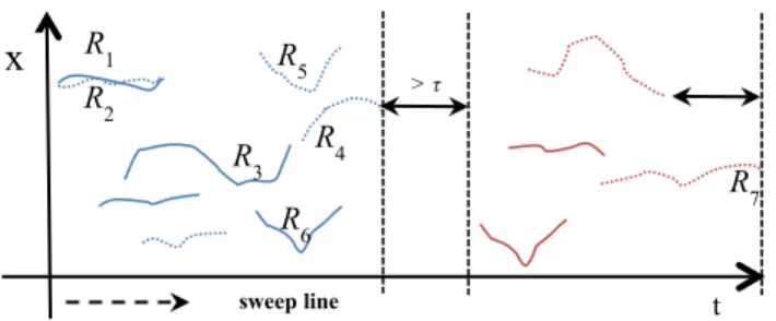
Given two representatives Ri and Rj if (a) the two representatives have the same lifespan with respect to threshold τ and (b) the two representatives are also similar w.r.t. similarity threshold δ (this means that they origin from different sub-chunks), then this implies a ‘merge’ operation. On the other hand, if (a) Ri ends close to the timepoint when the Rj starts with respect to threshold t, (b) the Euclidean distance of the last point of Ri is close (with respect to a distance threshold d) to the first point of Rj, and (c) a sufficient number of the same moving objects are represented by both representatives (with respect to a percentage threshold γ), this implies an ‘append’ operation. Fig. 7 illustrates representatives of a chunk consisting of two chunks. A merge operation occurs between R1 and R2, whereas R5 and R6 will both be maintained in the final outcome although they have similar lifespans. An append operation occurs between R3 and R4.

Fig. 7 Representatives of a chunk with two sub-chunks (dashed vs. continuous polylines) organized in a temporal priority queue of two groups (blue vs. red polylines)

Algorithm QuT-Clustering provided in Fig. 8 proposes such a solution on top of ReTraTree. The user gives as parameters the period of interest W, and the algorithm traverses the tree and returns clusters valid in this period. t

x

Algorithm QuT-Clustering

Input: ReTraTree root, temporal period W Output: Clusters C valid inside W 1. Hß{Hi, | overlap(root.Hi, W)}

2. for each Hi ∈ H do

3. Hi,n ß{Hi,n, | overlap(W, Hi,n.per)}

4. TEQ_PQßbulk_push_TEQ(TEQ_PQ, Hi,n, τ)

5. while TEQ_PQ ≠ Ø do

6. R ß temporal_interleaving(R ∪ TEQ_PQ.pop()) 7. for each Rj ∈ R do

8. Roverlap ß temporal_overlap(Rj, R, t)

9. for each Rk∈ Roverlap do

10. if (non_common_lifespan(Rj, Rk) < τ) then

11. if (𝑎𝑣𝑔 𝑉!!

!! _{≥ δ) then} 12. merge(Rj, Rk)

13. else if (|Rj,t.e – Rk,t.s| < t) then

14. if (euclidean_dist(p(Rj,t.e), p(Rk,t.s)) < d) AND (common_IDs(Rj, Rk) > γ) then

15. append(Rj, Rk)

16. else 17. continue

18. Rclusteredß{Rj ∈ R, | |Rj,t.e - Hi,t.e| > τ}

19. RßR-Rclustered

20. CßC ∪ Rclustered

21. return C

Fig. 8QuT-Clustering algorithm

More specifically, the algorithm initially finds the chunks and then the sub-chunks that overlap the given period (lines 1-3). These sub-chunks are organized in a priority queue (line 4), which orders groups of representatives of the sub-chunks. Each group contains temporally successive representatives that are at most in temporal distance τ from each other. To exemplify this ordered grouping of sub-chunks, Fig. 7 shows the

representative sub-trajectories (excluding outliers) of a single chunk, which consists of two sub-chunks, distinguished as dashed vs. continuous polylines. Note that for simplicity, y-dimension is omitted and specific borders of sub-chunks are not depicted, while the representatives form two groups, colored blue and red, respectively. Subsequently, the algorithm pops each group one-by-one and sorts all representatives with respect to time dimension, by interleaving the already sorted (from the step that constructs the priority queue) representatives coming from different sub-chunks (line 6). This is done by including representatives left from a previous round of the algorithm. Then, the algorithm sweeps the temporally interleaved representatives along the time dimension (line 7) and, for each of them, identifies the subset of its subsequent representatives in time that their lifespan overlap with the lifespan of the currently investigated representative, after the extension of the latter towards the future by t timepoints. For each pair of representatives Rj and Rk, the algorithm checks whether a merge operation (lines 10-12) or an append operation (lines 13-15) is necessary. In any other case (line 17) the algorithm simply continues with the next representative, and maintains both representatives intact. After each sweep, the algorithm maintains in the next round only those representatives that end at most τ

seconds before the border of the current chunk (e.g. R7, in Fig. 7), as candidates for merging with subsequent representatives (lines 18-20). The rest of the representatives are part of the final outcome of the algorithm. Regarding the technical details, a ‘merge’ operation practically maintains (in the working set of representatives R) one of the two representatives (e.g. the first) in the remaining process. The other representative is appropriately flagged so as to be able to retrieve the raw data that correspond to this cluster, if needed. For the ‘append’ operation, we need to retrieve the identifiers of the trajectories (not the sub-trajectories themselves) that correspond to the clusters implied by the representatives and apply a set intersection operation. This is facilitated by traditional indexing structures, such as by indexing the pair of representative id (i.e. cluster identifier) and sub-trajectory id of the raw data relation at the 4th _{level of} ReTraTree. Practically, an ‘append’ procedure replaces from the working set of representatives S the two representatives with one of those sub-trajectories that exist in both clusters. Note that the chosen sub-trajectory is selected randomly and it is the one used in the remaining process. Using another non-random choice at this step would be possible but not desired, as it would imply retrieval of the actual sub-trajectories. Finally, note that for simplicity reasons, we use the same threshold τ to compute the equivalence classes, as well as for considering whether two representatives refer to the same temporal period. In practice, these two easily configured parameters may be different, depending on the analysis scenarios pursued by the user. Similarly, threshold t corresponds to a small duration value, for instance, t = 0 in order to be as strict as possible.

4.2 Architectural aspects

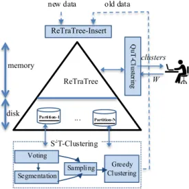
The architecture of our framework is illustrated in Fig. 9. The core of the framework is the ReTraTree structure that is fed by either new incoming trajectories or data that have been processed in a previous round and could not be clustered. In both cases the ReTraTree-Insert algorithm handles the insertion. The trajectories are

partitioned according to the in-memory part of the structure and stored on disk-based partitions. The trajectories assigned to an existing representative trajectory) are archived on disk in clustered partitions. Instead, trajectories that were not clustered are organized on disk in an (intermediate) outlier partition. When the size of the partitions exceeds a threshold, the S2_{T-Clustering algorithm applies the Voting process upon which the} Segmentation of the trajectories takes place. The resulting sub-trajectories and their voting descriptors form the input of the Sampling module that selects new (i.e. non-existing) representatives that are back-propagated to the in-memory part of the ReTraTree. The new representative trajectories and the raw sub-trajectories form the input of the GreedyClustering module. If a sub-trajectory is clustered around a new representative, it is archived on disk. Otherwise it is an outlier and is re-inserted to ReTraTree, as it may now be accommodated in the index. This is due to its segmentation during the operation of S2_{T-Clustering, or due to the creation of new matching} sub-chunks or representatives in the index. Finally, the analyst uses the QuT-Clustering algorithm to perform interactive clustering analysis by providing different time windows W as input.

Fig. 9Architectural aspects of ReTraTree

4.3 Complexity Analysis

Concluding the discussion about our proposal, we provide a complexity analysis of (i) loading the ReTraTree structure and (ii) performing QuT-Clustering, according to the algorithms proposed so far. The assumption we make throughout our analysis is that the distribution of trajectories during the dataset’s lifetime is uniform; in other words, selecting two random timepoints, ti and tj, the number of trajectories being ‘alive’ at ti and tj, respectively, remains more or less the same. In real world datasets, we do not expect to find perfect compliance to this, but we believe that this is a realistic assumption.

Lemma 1: Under the uniformity assumption, the loading cost of the ReTraTree is:

𝒪 𝑝∙ 𝑇!∙𝑁+𝐻∙𝑅! ∙𝑙𝑜𝑔 𝑇!∙𝑁 𝐻∙𝑅

where 𝐻 is the average number of sub-chunks per chunk, 𝑅  is the average number of representative sub-trajectories per sub-chunk and 𝑇!  denotes the average number of trajectory points in a database consisting of N

trajectories.

Proof: Considering that 𝐻 is the average number of sub-chunks per chunk and 𝑅  denotes the average number of representative sub-trajectories per sub-chunk, ReTraTree can be considered as p balanced trees of h = 2 (excluding the root and the 3D-Rtrees found at the 1st _{and the 4}th _{level of the structure, respectively) with the} upper bound for the maximum number of leaves per tree being upper bounded by 𝐻∙𝑅. Given the above, each sub-chunk has an average size of 𝑇!∙𝑁 𝐻∙𝑅 segments. Setting threshold α of each sub-chunk to this value,

ReTraTree will invoke the S2T-Clustering algorithm 𝒪(𝑝∙𝐻∙𝑅) times [result 1].

Regarding the cost of S2_{T-Clustering algorithm, it is composed by the costs of its two components, namely} Sampling and Greedy-Clustering (see Fig. 4). As it has been shown in (Panagiotakis et al. 2012), the most computationally intensive part of the Sampling method is the voting process with 𝒪 𝑇!∙𝑁∙𝑙𝑜𝑔 𝑇!∙𝑁 cost

for each trajectory in a database consisting of N trajectories indexed by a 3D-Rtree structure. Note that in our case, we maintain a forest of such trees, where each of them corresponds to the segments of the sub-trajectories that belong to the dynamically changing set of outliers of a sub-chunk. Therefore, in our case the number N of trajectories corresponds to the number of sub-trajectories that have been assigned to this set. Regarding Greedy-Clustering, as the voting vectors are pre-calculated during the Sampling step, its cost is dominated by the size of the representatives set 𝑅. More specifically, the cost is 𝒪 𝑅∙𝑙𝑜𝑔 𝑇_!∙𝑁 , i.e. the cost of performing 𝑅

trajectory-based range queries in the database [result 2].

Voting Segmentation Sampling Greedy Clustering S2_T-Clustering Parti ti on-1 ...

new data old data

W disk memory Partition-N ReTraTree clusters Q uT -C lus ter ing ReTraTree-Insert

Since the size of the outliers of a sub-chunk set is estimated to be 𝑇!∙𝑁 𝐻∙𝑅, the cost of the S2T-Clustering

algorithm in a sub-chunk is: 𝒪 𝑇!∙𝑁 𝐻∙𝑅∙𝑙𝑜𝑔 𝑇!∙𝑁 𝐻∙𝑅 +𝑅∙𝑙𝑜𝑔 𝑇!∙𝑁 𝐻∙𝑅 [result 3].

By combining results 1-3 above (i.e. multiply the 𝑝∙𝐻∙𝑅 number of leaves with the cost of the S2 T-Clustering algorithm of a single sub-chunk), we have proven Lemma 1. n

From a different point of view, the cost per trajectory insertion can be split in four parts: (i) the cost of chunking and sub-chunking the original trajectory to sub-trajectories, (ii) for each sub-trajectory, the cost of finding the matching representative, (iii) the cost of invoking the S2_{T-Clustering algorithm, which is only in} case that the sub-trajectory overflows threshold α of the sub-chunk, and (iv) the cost of checking whether the new representatives extracted by S2T-Clustering can be inserted into the already identified representatives. Regarding the cost of each part, that of (i) is trivial, while that of (ii) and (iv) is 𝒪(R) in both cases, since it implies a scan on the set of representatives, which however is small (R<<N). Obviously, the cost per trajectory insertion is dominated by the S2T-Clustering algorithm.

Lemma 2: Under the uniformity assumption, the cost of the QuT-Clustering algorithm is:

𝒪 𝐻∙𝑅 !

where 𝐻 is the average number of sub-chunks per chunk and 𝑅  is the average number of representative sub-trajectories per sub-chunk.

Proof: As already shown, under uniformity assumption, each chunk maintains 𝒪(𝐻∙𝑅) representatives. Thus, invoking QuT-Clustering will eventually scan a number of 𝒪(|𝑊| _𝑝 ∙𝐻∙𝑅) representatives, where

|𝑊|

𝑝 is the number of the involved chunks. However, at any time, the algorithm maintains a priority queue of 𝒪(𝐻∙𝑅) representatives (worst case scenario). Note that sorting this priority queue costs 𝒪(𝐻∙𝑅) only, since the sets of representatives of the corresponding sub-chunks are already sorted, thus a merge-sort performs the required temporal interleaving. Given this, as the representatives reside in memory and there is no special organization at this level, for each of these representatives the algorithm will scan all the other representatives in the worst case, thus leading to 𝒪( 𝐻∙𝑅 !_{) cost. n}

Interestingly, the cost of the QuT-Clustering algorithm is independent to the size of the database, thus it is a highly efficient solution for progressive temporally-constrained sub-trajectory clustering analysis. This is validated in the experimental study that follows.

5.

Experimental Study

In this section, we present our experimental study. ReTraTree and its algorithms were implemented in-DBMS in Hermes2 _{MOD engine over PostgreSQL, by using the GiST extensibility interface provided by PostgreSQL.} More specifically, the top three levels of ReTraTree that reside in memory were implemented as temporary tables, while the 4th level was stored in traditional tables, upon which the 3D-Rtrees were built. Although our proposal is generic, we chose to put extra effort to implement it on a real-world MOD management system rather than an ad hoc implementation, because of the initially placed goal to support progressive clustering analysis. We argue that this is an important step towards bridging the MOD management and mobility mining domains, as state-of-the-art frameworks (Giannotti et al. 2011) could make use of the efficiency and the advantage of our proposal to execute clustering analysis tasks via simple SQL. This way, our approach becomes practical and useful in real-world application scenarios, where concurrency and recovery issues are taken into consideration.

All the experiments were conducted on an Intel Xeon X5675 Processor 3.06GHz with 48GB Memory running on Debian Release 7.0 (wheezy) 64-bit. We used PostgreSQL 9.4 Server with the default configuration for the memory parameters (shared_buffers, temp_buffers, work_mem, etc.). The outline of our experimental study is as follows: in Section 5.1, we discuss the setting of various parameters. In Section 5.2 we present baseline solutions with which we compare our proposals. In Section 5.3 we describe the datasets that we used in this study. In Section 5.4, we apply a qualitative analysis to verify that our proposal operates as expected by using datasets with ground truth. In Section 5.5 we provide a sensitivity analysis with respect to various parameters. In Section 5.6 we continue the qualitative evaluation of our approach in real datasets with general-purpose clustering validation metrics. In Section 5.7, we evaluate the maintenance of ReTraTree in terms of loading performance and size. In Section 5.8, we measure the I/O performance of ReTraTree with respect to the QuT-Clustering algorithm, the performance of which is assessed in Section 5.9.

5.1 Parameter settings

Regarding parameter settings, as our approach makes use of the sampling methodology of (Panagiotakis et al. 2012), we followed the best practices presented in that work. More specifically, the value of parameter σ was set to 0.1% of the dataset diameter, while that of ε was set to 10-3. We would like to note that we made several

experiments by modifying the values of these parameters and the differences in the results were negligible, thus in a way we re-validated our earlier experience in the current setting.

As far as it concerns the parameters that affect the construction of ReTraTree, their effect is rather straightforward. Here we report our findings, which have been experimentally validated. More specifically, the more we increase p, the more chunks we create and hence the more the partitions (i.e. relations in our implementation). As the number of these partitions increases, the size and the construction time of ReTraTree decreases as the structure holds the same amount of data, but in smaller relations (i.e. smaller indexes). Moreover, as by increasing p we have a smaller structure size, the runtime of QuT-Clustering will be smaller. Regarding the τ parameter, the smaller it is, the more the number of sub-chunks and hence the more relations; thus, we fall at the previous case. In addition, the smaller the similarity threshold δ, the more the sub-trajectories that are assigned to already existing clusters. This implies that fewer sub-trajectories will end up to the outliers’ set and hence the S2T-Clustering algorithm runs fewer times. This means that the lower the δ the lower the construction time of the ReTraTree. Finally, regarding the value of α that is the threshold of the size of the outliers’ set above which the S2T-Clustering algorithm is applied, the more we increase α, the fewer times the S2_{T-Clustering will run and consequently the smaller the construction time of ReTraTree. In our experiments we} fixed threshold α to 5% of the dataset size.

In the subsequent sections we report on the effect of the important parameter of the time window W, while in Section 5.5 we particularly study the effect on both the efficiency and the quality of QuT-Clustering when varying the values of the remaining parameters, whose effect is not trivial to foresee without experimentation. 5.2 Baseline solution

To the best of our knowledge the ReTraTree structure and the corresponding QuT-Clustering algorithm is a novel solution to the temporally-constrained sub-trajectory cluster analysis problem and there is no comparable technique. Furthermore, as already mentioned, the S2T-Clustering algorithm has some unique characteristics that make it appropriate as part of our solution. The most important characteristic is that it provides a greedy solution to the problem for the degenerated case where the time window W is equal to the entire lifespan of the dataset. This is a key observation that we exploit in our approach by organizing our data in sub-chunks consisting of sub-trajectories having the same lifespan and applying S2T-Clustering to them. In Section 5.3 we demonstrate that the state-of-the-art TRACLUS algorithm (Lee et al. 2007) that is utilized also by the TCMM framework (Li et al. 2010b) cannot identify the clusters in datasets including ground truth. Moreover, in (Panagiotakis et al. 2012) it is shown that an efficient solution for the sampling process that the S2_{T-Clustering algorithm utilizes, it} requires a 3D-Rtree index.

Given the above, in this empirical study we set the following comparable pairs: (i) we compare the ReTraTree structure with the Rtree structure. A secondary but important reason for this choice is that 3D-Rtree is the prevailing structure that state-of-the-art spatial DBMS vendors have chosen to support in their products (e.g. PostGIS, Oracle Spatial); (ii) we compare the S2_{T-Clustering algorithm with QuT-Clustering} algorithm for the degenerated case where the time window W is equal to the entire lifespan of the dataset. Of course, our approach is applicable in any user-defined time window W. Thus, in this case the comparable pair is on the one hand the QuT-Clustering and on the other hand again the S2T-Clustering algorithm after having restricted the dataset to the selected time window W. This implies that an analyst should first apply a temporal range query to restrict the dataset inside W, then build a 3D-Rtree on the restricted dataset and afterwards run the S2T-Clustering algorithm. This is the best choice to perform a progressive clustering analysis without the ReTraTree and this is how the analysts work currently.

5.3 Datasets

In this study we used two real datasets (IMIS and GeoLife) and one synthetic (called SMOD); Table 2 presents their statistics3.

IMIS - IMIS is a real dataset consisting of the trajectories of 2,181 ships sailing in the Eastern Mediterranean for one week; data are collected through the Automatic Identification System (AIS) through which ships are obliged to broadcast their position for maritime regulatory purposes.

GeoLife - the GeoLife dataset (Zheng at el. 2010) contains 18,668 trajectories of 178 users in a period of more than four years. This popular dataset represents a wide range of movements, including not only urban transportation (e.g. from home to work and back) but also different kinds of activities, such as sports activities, hiking, cycling, entertainment, sightseeing and shopping.

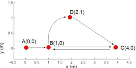
SMOD - Synthetic MOD (SMOD) consists of 400 trajectories and is used solely for the ground truth verification. The creation scenario of the synthetic dataset is the following: the objects move upon a simple graph that consists of the following destination nodes (points) with coordinates A(0, 0), B(1, 0), C(4, 0), and D(2, 1) illustrated in Fig. 10.

3_{The GeoLife dataset is publicly available. The other two datasets are publicly available at chorochronos.datastories.org repository under the}

Figure 10. The 2-D map of SMOD with the three one-directional and one bidirectional road

We assume that half of the objects move with normal speed (i.e. 2 units per second) and the rest of them move with high speed (i.e. 5 units per second). To be more realistic, we have also added 50 db Gaussian white noise to the spatial coordinates of SMOD. The objects move under the following scenario (rules), for a lifetime of one hundred seconds: There exist three one-directional roads (A → B, B → D, D → C) and one bi-directional road (B ⇆ C). At t = 0 sec, all objects start from point A. Thus, the first destination of all objects is point B. Since half of the objects move with different speed, half of them (i.e. 200 objects) will arrive to point B at t = 20 sec and the rest of them at t = 50 sec.

When an object arrives at a destination point, it ends its trajectory with a probability of 15%. Otherwise, it continues with the same speed to the next point. If there exist more than one possible next point, it decides randomly about the next destination.

Table 2: Dataset Statistics

Statistic SMOD IMIS GeoLife

# Trajectories 400 2,181 18,668

# Segments 35,273 12,516,337 24,159,325

Dataset duration 100 sec 7 days ~5 years

Avg. segment length (m) 8 169.5 72

Avg. segment speed (m/sec) 7.8 6 5

Avg. sampling rate (sec) 1 37 4

Avg. trajectory speed (m/sec) 2.9 3.7 3.9

Avg. # points per trajectory 89 5,739 1,295

Avg. trajectory duration 1.5 min 2.8 days 2.7 hours

Avg. trajectory length (km) 0.7 972.4 93

5.4 Quality of clustering analysis in synthetic datasets including ground truth

To the best of our knowledge there is no real trajectory dataset that provides ground truth that can be utilized for validating clustering techniques. Thus, our premise is to evaluate our approach qualitatively by using a synthetic dataset. The description of SMOD implies that the possible ending times of a moving object are t ≈ 20, t ≈ 50, t ≈ 80 or t ≈ 100. Based on this fact and by setting the chunk size equal to the duration of the dataset (i.e. 100 sec) we infer that the ReTraTree construction process should create 4 sub-chunks. We also infer the lifespan l of each sub-chunk. The invocation of the ReTraTree-Insert that builds these sub-chunks, concludes to apply the S2_{T-Clustering algorithm in each of these sub-chunks, which in its turn results in discovering representatives} (i.e. clusters) in each of them. This ground truth is illustrated in Table 3.

Table 3. The ground truth in SMOD

Sub-chunk Path Time periods (clusters)

H1,1 l = [0, 100] A→B [0, 20], [0, 50] B→C [20, 80], [50, 100] B→D [20, 52], [50, 100] C→B [80, 100] D→C [52, 100] H1,2 l = [0, 80] A→B [0, 20], [20, 80] B→C [20, 80] H1,3 l = [0, 50] A→B [0, 20] [0, 50] B→D [20, 52] H1,4 l = [0, 20] A→B [0, 20]

For instance, sub-chunk H1,1 with lifespan [0, 100] (i.e. objects that move through out the dataset’s lifespan) includes eight representatives, for each of which we note its lifespan. For example, in H1,1 there are two sub-trajectory clusters on the path A→B, with lifespans [0, 20], [0, 50], respectively.

We have loaded the SMOD dataset to the ReTraTree. We set the temporal tolerance parameter to τ = 2 (i.e. we impose 1 second difference in the starting/ending timepoints). The resulting ReTraTree discovered indeed four sub-chunks with lifespans: [0, 100], [0, 81], [0, 54] and [0, 20]. By incrementally applying S2_T-Clustering in each of them, we resulted in the discovery of the representatives. Fig. 11 illustrates the representatives of the

four sub-chunks. By combining each row in Table 3 with Fig. 10(a)-(d), we conclude that ReTraTree discovers the correct representatives, with their lifespans only slightly deviating from ground truth.

(a) (c)

(b) (d)

Fig. 11 The representatives of the four sub-chunks

We now investigate how the QuT-Clustering algorithm would operate by setting the temporal period W e.g. to the whole lifespan of the dataset. We used the values 5 sec, 10 m and 50% for (t, τ), d and γ respectively. After all append and merge operations take place, the resulting representatives are depicted in Fig.12, which is almost identical to the expected ground truth.

Figure 12: QuT-Clustering results with W=[0, 100]

In order to measure the stability of our method to noise effects, we have added more Gaussian white noise with Signal to Noise Ratio (SNR) level SNR = 30 db. The initial SMOD with additive noise of SNR = 50 db and the new SMOD with SNR = 30 db projected in 2-D spatial and 3-D spatiotemporal space is illustrated in Fig. 13. A small number of objects (i.e. outliers, four in our experiment) randomly move in space other than the roads that the other objects reside. These are also depicted in Fig. 13. In addition, the speed of outliers is updated randomly. Furthermore, for the sake of simplicity we assume that the chunk size is the whole lifespan of the dataset. According to this, the ground truth is restricted to the eight different paths that are valid for sub-chunk H1,1.

Figure 13: The trajectories of the SMOD with additive noise of SNR = 50 db projected in (a) 2-D spatial space ignoring time dimension and (b) spatiotemporal 3-D space. The trajectories of the SMOD with additive noise of SNR = 30 db projected in (c) 2-D spatial space and (d) spatiotemporal 3-D space. (e) The four outliers of the SMOD with additive noise of SNR = 50 db projected in 2-D spatial space ignoring time dimension. (f) The four outliers of our synthetic MOD with additive noise of SNR = 30 db projected in 2-D spatial space.

Given the above, and in order to demonstrate the benefits of S2T-Clustering we compare with TRACLUS (Lee et al. 2007), the state-of-the-art sub-trajectory clustering technique. Again we assume that the chunk size is the whole lifespan of the dataset, hence the ground truth restricts to the eight different paths that are valid for sub-chunk H1,1. In Fig. 14(a) and (b), we present the results of the S2T-Clustering and TRACLUS, respectively. Specifically, in Fig. 14(a) we depict the selected sub-trajectories by S2T-Clustering to serve as the pivots (i.e. representatives) for grouping other sub-trajectories around them, while in Fig. 14(b) we depict the synthesized representatives extracted (with RTG algorithm (Lee et al. 2007)) after the TRACLUS’s grouping phase. Based on this experiment, it turns out that S2_{T-Clustering effectively discovers all eight clusters (as well as the noisy} sub-trajectories), thus S2T-Clustering is not affected by the trajectories’ shape, yielding an effective and robust approach for the discovery of linear and non-linear patterns. On the contrary, TRACLUS fails to identify the hidden ground truth in this SMOD (i.e. it discovers only four out of the eight clusters) due to the fact that it ignores the time dimension. Interestingly, note that TRACLUS discovers more or less linear patterns, ignoring the temporal information of the trajectories, as mentioned in (Lee et al. 2007).

(a) (b)

Figure 14: The representative trajectories (i.e. clusters) discovered by (a) S2_{T-Clustering(b) TRACLUS}

In order to evaluate the accuracy of our proposal in a quantified way, we further employed F-Measure in SMOD. In detail, we built 8 datasets, with the first consisting of the trajectories of the first cluster of sub-chunk H1,1 only, the second consisting of the sub-trajectories of the first and the second cluster only, and so on, until the eighth dataset, which consisted of the sub-trajectories of all eight clusters. All eight datasets appeared in two variations: including or not the set of outliers. For each dataset, we applied S2T-Clustering and calculated F-Measure; Fig. 15 illustrates this quality criterion by increasing the number of clusters. It is evident that S2 T-Clustering turns out to be very robust, achieving always precision and recall values over 92.3%, while the outliers are always detected correctly.