Generation of Synthetic Data Sets for Evaluating the
Accuracy of Knowledge Discovery Systems
Daniel R. Jeske
University of California
Department of Statistics
Riverside, CA 92521
1-951-827-3014
[email protected]
Behrokh Samadi
Lucent Technologies
Performance Analysis Department
Holmdel, NJ 07733
1-408-872-1886
[email protected]
Pengyue J. Lin
Lan Ye, Sean Cox, Rui Xiao
Ted Younglove, Minh Ly
Doug Holt, Ryan Rich
University of California,
Riverside CA
ABSTRACT
Information Discovery and Analysis Systems (IDAS) are designed to correlate multiple sources of data and use data mining techniques to identify potential events that could occur in the future. Application domains for IDAS are numerous and include the emerging area of homeland security.
Developing test cases for an IDAS requires background data sets into which hypothetical future scenarios can be overlaid. The IDAS can then be measured in terms of false positive and false negative error rates. Obtaining the test data sets can be an obstacle due to both privacy issues and also the time and cost associated with collecting multiple instances of a diverse set of data sources.
In this paper, we give an overview of the design and architecture of an IDAS Data Set Generator (IDSG) that will enable a fast and comprehensive test of an IDAS. The IDSG will generate data using syntactical rule-based algorithms and also semantic graphs that represent interdependencies between attributes. The IDSG tool will feature a default set of attribute generation capabilities as well as a wizard that allows users to grow the scope of data the tool can generate. We describe the data generation algorithms for some default attributes such as name, gender, age, address, phone number, driver’s license number, social security number, credit card number, income level, occupation, and credit card transactions. The credit card transaction example illustrates the use of semantic graphs to capture attribute dependencies, and also illustrate our approach for approximating high dimensional multivariate distributions.
Categories and Subject Descriptors
D.2.5 [Testing and Debugging]: Testing Tools. D.2.4 [Software/Program Verification]: Statistical Methods, Validation. I.2.4 [Knowledge Representations Formalisms and Methods]: Semantic Graphs.
General Terms
Algorithms, Design, Verification
Keywords
Information Discovery, Data Mining, Data Generation.
1.
INTRODUCTION
1.1
Background
Modern data collection methods in combination with the rapid increases in information technology have made possible the assembling of extensive data sets on individuals. Information Discovery and Analysis Systems (IDAS) form an important tool for turning large quantities of data that have been collected into
information that can be used. IDAS’s are designed to correlate
multiple sources of data and use data mining techniques to find relationships within disparate data sets that could be used to predict events that occur in the future. An IDAS extracts information from data by finding patterns, threads, and relationships. To do this, IDASs use a hybrid of statistical and artificial intelligence methodologies such as pattern recognition, classification, categorization, and learning, and employ data mining tools based on neural networks, Bayesian networks, classifications schemes, and regression models, among others, to cull out and aggregate information across different data sources. IDAS’s have been a major asset to business applications such as fraud prevention [2,7] and are in use in the medical field in a wide variety of applications including help in diagnosis [5] and analysis of medical videos [13].A recent survey by the US General Accounting Office found that 52 federal agencies are conducting or plan to conduct 199 separate data mining efforts, with 131 of these currently operational [4]. It is believed that IDAS’s could be equally effective for intelligence applications such as providing leading indicators of terrorist acts.
1.2
Motivating Problem
A critical technical issue with IDASs is their ability to provide accurate inference. Given the diversity of techniques used to develop an IDAS, it is desirable to have a baseline approach for testing their ability to make accurate inference as well as their ability to deal with large input data sets with varying degrees of accuracy. An important part of testing of IDAS’s is the generation of synthetic data sets for use in test cases.
Developing test cases for an IDAS requires background data sets into which hypothetical future scenarios can be overlaid. The IDAS can then be measured in terms of false positive and false negative error rates. Obtaining the test data sets can be an obstacle due to both privacy issues and also the time and cost
associated with collecting multiple instances of a diverse set of data sources.
In this paper, we give an overview of the design and architecture of an IDAS Data Set Generator (IDSG) that will enable a fast and comprehensive test of an IDAS. This IDSG is currently under development for the Department of Homeland Security (DHS) by the University of California, Riverside and Lucent Technologies. The specific goal is to design and develop a prototype system to explore the feasibility of synthesizing data sets for testing the effectiveness of IDASs designed to uncover potential threat scenarios. Such a data synthesis capability is an attractive alternative for testing an IDAS when realistic data sets are not readily available due to privacy or restrictive access issues, or the challenge and costs of amassing diverse data from multiple sources is imposing. Further, a synthetic data capability allows various features and capabilities of an IDAS to be exercised in multiple test cases, thus permitting a meaningful figure of merit of its efficacy to be established.
There are several difficulties in the generation of IDAS test data in general, and for the DHS project in particular.
General difficulties include:
• Multivariate data – IDASs use large numbers of data fields with unknown correlations between fields.
• Multiple data types – Data for these systems can be continuous, nominal, ordinal, textual, or image data.
• Lack of available high dimension data – Readily available data, the type needed to quickly develop test cases, typically are presented in two or at most three dimensions. DHS specific difficulties include:
• Privacy issues –The Department of Defense, Office of the Inspector General issued a report finding that the Defense Advanced Projects Agency (DARPA) had not adequately considered privacy concerns associated with the Total Information Awareness Program terrorism data mining project [3].
• Security issues – The need to maintain security for the DHS precludes the direct interaction with the client to identify relevant data fields.
• Lack of training data – Because of security needs, training data for evaluating the effectiveness of the data synthesis tools are not available.
The problem of developing a data set generator that can create realistic data for all possible IDAS data input types for all possible IDASs is formidable, and really is not our goal. Instead, our approach is to synthesize data sets of sufficient quality to enable IDAS evaluation. Our vision is an experimental platform that generate data sets containing user-designed threat scenario information as well as background data whose quality can be increased as needed by imposing relationships, correlations, and other statistical conditions on the data attributes within or across data sets.
1.3
Objective
Examples of generation of synthetic data through various means for testing purposes are available in many areas of research. For example, synthetic data sets were generated for testing a Robust/Resistant crystallographic refinement procedure using two sets of Gaussian random errors, a Gaussian error distribution contaminated with 10% drawn from a high variance Gaussian distribution, and a long-tailed random error distribution [8]. Synthetic data has been generated for use in “ground truth” testing of different protein spot detection software packages through the use of a Gaussian mixture model obtained from training data [9]. Synthetic handwriting data have been generated using random perturbations of actual handwriting for use in testing cursive hand-writing recognition systems [10]. Alternatively, the US Census Bureau is exploring the use of synthetic data as a means of protecting the confidentiality of the public while maintaining statistical quality [1].
In multivariate cases, particularly where there are complex covariance structures requiring an understanding of the interdependencies between variables, the data synthesis process becomes more complex. Central to the approach in this paper is the development of an object-oriented information model to represent data objects that readily permit imposing additional data structure and conditions on data attributes.
Our synthetic data generation design is based on the use of semantic graphs. For this project, a semantic graph is defined as a graphical depiction of the interrelationships between data fields of interest. Semantic graphs have been used in various fields for summarizing complex relationships between multiple factors. For example, document summaries have been produced using semantic sub-graphs to represent the various characteristics of the document but in a vastly reduced size [6]. Complex relationships between pairs of nouns in sentences have been summarized using automatic graph algorithms [11] as well.
A key aspect of our objective to synthesize evaluative IDAS input data is to provide a scalable design that can be adapted to increase data quality, add data types, and address computational constraints dictated by our users.
The rest of this paper is organized as follows. Section 2 describes the general architecture used in our data generation approach. Section 3 provides a few illustrative applications of our proposed design, with an example drawn from generating credit card transaction data. Section 4 summarizes the principal findings to-date of this project.
2.
ARCHITECTURE
2.1
User Scenario
To better demonstrate the functionality of IDSG, we present a ‘typical’ user scenario in Figure 1. As shown in the figure, the user initially enters information on the type of data set, tables, table relationships, the attributes within each table, and the attribute relationship.
Figure 1. A Typical User Scenario
At this point, the user needs to define the relationships amongst the attributes. This will be done by a SematicGraphBuilder. As an example, for a credit card transaction data set, the user may require two tables, CardHolder and CardTransaction, with 1-to-many relationship between the CardHolder and the CardTransaction Tables.
The table CardHolder has attributes: Name, Address, TelephoneNumber, Date-of-Birth, Gender, Income, CardNumber, CustomerSinceDate. CardTransaction table includes attributes CardNumber, TransactionDate, Transaction Amount, PurchasedItem, and BusinessName.
For selection of the attributes, the user will be provided with a set of pre-defined attributes to choose from. However, if desired, an IDSG Wizard will allow the user to define new attributes. Once the above two sets of information are provided, IDSG may build the DataSetSchema. For the schema, the user needs to input the multiplicity relationship between the tables. In this example, the user needs to specify how many transaction records per CardHolder/card to generate. For this, IDSG will provide a list of probability distributions to select from.
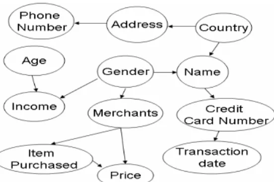
On the screen a partially constructed semantic graphs will appear (Figure 2). The graph is partially constructed since some of the attributes or relationships may not have been predefined and thus need to be specified by the user. For example, the relationship between Age and Income may already exist, but the user may decide to add an additional relationship between Gender and Income. This will add an additional link to the semantic graph between the Gender and Income attributes and open a window for specification of the type of relationship. Alternatively, the user may determine to maintain the structure of the graph (nodes and edges) and only modify parameters. For example, the user may decide to change the parameters for Gender distribution from 50-50 to 40-60, if the number of Male-Female credit card holders are a 40-60 ratio.
Figure 2. A Partially Constructed Semantic Graph
Once the schema and the semantic graph are represented, the user provides the information on other parameters. For example, the number of records in each table, the duration of time for the events, the geographic area (for addresses), the nationality (for names), and the type of items purchased (eg, airline, hotels, and car rentals only). The above parameters further constrain the type of data generated. Once these parameters are input, the IDSG data generator module can generate the data sets and store them in some specific format. Initially, this format is a comma separated file.
2.2
Semantic Graphs and Related Tables
A key step in our methodology is the use of a semantic graph to represent dependency relationships among different data sets. While semantic graphs typically are used to summarize pre-existing data, in our methodology the semantic graph serves as a guide for the creation of the synthetic data. The semantic graph is also used to illustrate the data generation sequence to be used in the synthesizing process.The first phase of the data generation process is the construction of the semantic graph. A key assumption in our methodology is that semantic graphs can adequately capture the relationships within the data. The IDSG tool uses a semantic graph that describes these data relationships. The basic elements of our semantic graphs are data attributes and directed dependencies. Ovals in the semantic graph represent various data attributes, and arrows indicate the dependency relationship between two data attributes. The number of arrows coming into a data attribute dictates the dimension of an inner table that holds information about conditional probability distributions for the data attribute. The conditional distribution of the data attribute is theoretically specified once the values of all of the upper level data attributes are known.
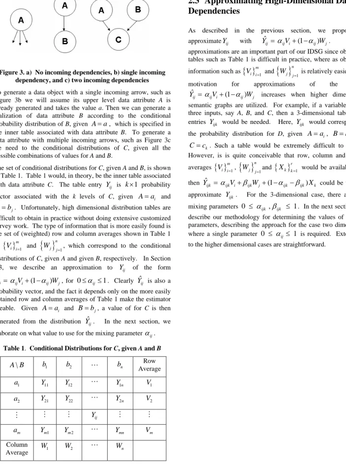
Data attributes without incoming arrows such as illustrated in Figure 3a will be assigned a distribution from either the system or the user. Since this type of data object does not have incoming arrows, they are independent of other data attributes. The generation of this type of data attribute is done with simple random sampling.
Figure 3. a) No incoming dependencies, b) single incoming dependency, and c) two incoming dependencies
To generate a data object with a single incoming arrow, such as Figure 3b we will assume its upper level data attribute A is already generated and takes the value a. Then we can generate a realization of data attribute B according to the conditional probability distribution of B, given A=a, which is specified in the inner table associated with data attribute B. To generate a data attribute with multiple incoming arrows, such as Figure 3c we need to the conditional distributions of C, given all the possible combinations of values for A and B.
The set of conditional distributions for C, given A and B, is shown in Table 1. Table 1 would, in theory, be the inner table associated with data attribute C. The table entry
Y
ij isk
×
1
probability vector associated with the k levels of C, givenA
=
a
i andj
B
=
b
. Unfortunately, high dimensional distribution tables are difficult to obtain in practice without doing extensive customized survey work. The type of information that is more easily found is the set of (weighted) row and column averages shown in Table 1 as{ }
1 m i iV
= and{ }
1 n j j W= , which correspond to the conditional
distributions of C, given A and given B, respectively. In Section 2.3, we describe an approximation to Yij of the form
ˆ (1 )
ij ij i ij j
Y
=
α
V+ −
α
W , for0
≤
α
ij≤
1
. Clearly Yˆ
ij is also aprobability vector, and the fact it depends only on the more easily obtained row and column averages of Table 1 make the estimator useable. Given A
=
ai and B=
bj, a value of for C is then generated from the distribution Yˆ
ij. In the next section, we elaborate on what value to use for the mixing parameterα
ij.Table 1. Conditional Distributions for C, given A and B
\
A B
b1 b2 bn Row Average 1 a Y11 Y12 Y1n V1 2 a Y21 Y22 Y2n V2 ijY
m a Ym1 Ym2 Ymn Vm Column Average 1 W W2 Wn2.3
Approximating High-Dimensional Data
Dependencies
As described in the previous section, we propose to approximateYij with Y
ˆ
ij=
α
ijVi+ −
(1
α
ij)
Wj. Theseapproximations are an important part of our IDSG since obtaining tables such as Table 1 is difficult in practice, where as obtaining information such as
{ }
1 m i iV
= and{ }
1 n j j W= is relatively easier. The
motivation for approximations of the form
ˆ
(1
)
ij ij i ij j
Y
=
α
V+ −
α
W increases when higher dimensional semantic graphs are utilized. For example, if a variable D has three inputs, say A, B, and C, then a 3-dimensional table with entries Yijk would be needed. Here, Yijk would correspond to the probability distribution for D, given A=
ai,B
=
b
j andk
C
=
c . Such a table would be extremely difficult to obtain. However, is is quite conceivable that row, column and planar averages{ }
1 m i iV
= ,{ }
1 n j j W = and{ }
1 r k kX
= would be available andthen Y
ˆ
ijk=
α
ijkVi+
β
ijkWj+ −
(1
α
ijk−
β
ijk)
Xk could be used toapproximate Yijk. For the 3-dimensional case, there are two mixing parameters
0
≤
α
ijk,
β
ijk≤
1
. In the next section, wedescribe our methodology for determining the values of mixing parameters, describing the approach for the case two dimensions where a single parameter
0
≤
α
ij≤
1
is required. Extensions2.3.1 Algorithm for Mixing Parameter
The weighted row and column averages shown in Table 1 are functions of weights derived from the joint distribution for A and
B, which is shown in Table 2. Here, pij=Pr (A=ai,B=bj).
Table 2. Joint Distribution of A and B
\
A B b1 b2 bn Marginal for A 1 a p11 p12 p1n p1i 2 a p21 p22 p2n p2i ij p m a pm1 pm2 pmn pmi Marginal for B 1 pi pi2 pinIt follows that the weighted row and column averages shown in Table 1 can be expressed as
1 2 1 2 1 2 1 2 , 1 , 1 j i i in i i i in i i i j j jm j j jm j j j p p p V Y Y Y i m p p p p p p W Y Y Y j n p p p = + + + ≤ ≤ = + + + ≤ ≤ i i i i i i
In general applications, the mn probability vectors Yij and
11 12
(
,
,
,
mn)
p
=
p p … p will not be known. We model theY
ijvectors as independent identically distributed k-dimensional uniform Dirichlet random vectors, and p as a mn-dimensional uniform Dirichlet random vector that is independent of all the
Y
ij. In some sense, our model corresponds to a Bayesian non-informative prior, though our use of the model is not within the typical Bayesian paradigm. Rather, we use this approach to define a structural characterization of theY
ij andp
ij values that we can optimize against. While we cannot expect the Dirichlet assumptions to hold across all applications, it can be argued that it is the most reasonable thing to do in the absence of any other information.For a given realization of
( { } ,
Yij p)
we can find the “optimal”value of
α
ij by minimizing the total error sum of squares2
(1
)
ij ij i ij j
Q
=
Y−
α
V− −
α
W . It is easy to show that the minimizingα
ij, over the interval (0,1) is the value( ) ( ) ˆ 1 , 0 , ( ) ( ) j ij j i ij j i j i W Y W V M in M a x W V W V α = ⎡⎢ ⎛⎜⎜ − ′′ − ⎞⎟⎟⎤⎥ − − ⎢ ⎝ ⎠⎥ ⎣ ⎦ .
The quantity ˆαij is a random variable, varying through the
Dirichlet distributions used for the Yij and p. The distribution
of ˆαij depends on m, n and k, but does not depend on either i or j. Our choice for the mixing parameter is the mean value of ˆαij,
which we obtain numerically by the following algorithm: 1) Simulate mn independent realizations of Yij from a k
-dimensional uniform Dirichlet distribution
2) Simulate a one realization of p from an mn-dimensional uniform Dirichlet distribution
3) Compute ˆαij
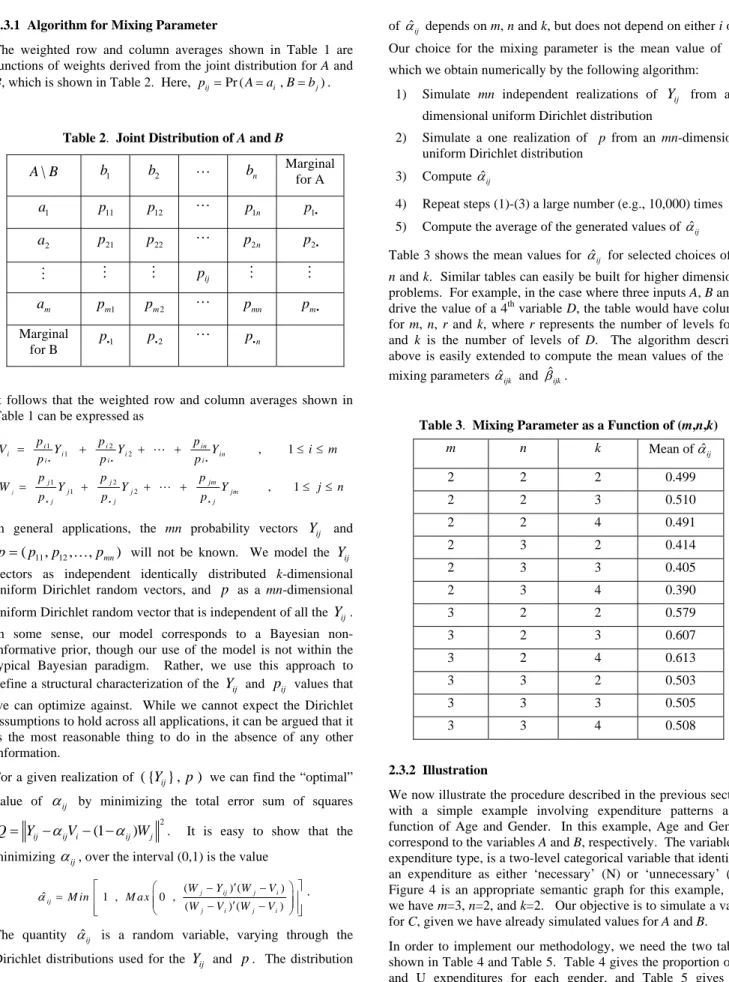
4) Repeat steps (1)-(3) a large number (e.g., 10,000) times 5) Compute the average of the generated values of ˆαij Table 3 shows the mean values for ˆαij for selected choices of m,
n and k. Similar tables can easily be built for higher dimensional problems. For example, in the case where three inputs A, B and C
drive the value of a 4th variable D, the table would have columns for m, n, r and k, where r represents the number of levels for C
and k is the number of levels of D. The algorithm described above is easily extended to compute the mean values of the two mixing parameters ˆαijk and ˆβijk.
Table 3. MixingParameter as a Function of (m,n,k)
m n k Mean of αˆij 2 2 2 0.499 2 2 3 0.510 2 2 4 0.491 2 3 2 0.414 2 3 3 0.405 2 3 4 0.390 3 2 2 0.579 3 2 3 0.607 3 2 4 0.613 3 3 2 0.503 3 3 3 0.505 3 3 4 0.508 2.3.2 Illustration
We now illustrate the procedure described in the previous section with a simple example involving expenditure patterns as a function of Age and Gender. In this example, Age and Gender correspond to the variables A and B, respectively. The variable C, expenditure type, is a two-level categorical variable that identifies an expenditure as either ‘necessary’ (N) or ‘unnecessary’ (U). Figure 4 is an appropriate semantic graph for this example, and we have m=3, n=2, and k=2. Our objective is to simulate a value for C, given we have already simulated values for A and B. In order to implement our methodology, we need the two tables shown in Table 4 and Table 5. Table 4 gives the proportion of N and U expenditures for each gender, and Table 5 gives the
proportion of N and U expenditures for each of the three age groups.
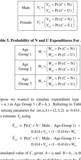
Table 4. Probability of N and U Expenditures For Gender
Male 1 11 12 Pr ( N) Pr ( U) V C V V C = = ⎛ ⎞ = ⎜ = = ⎟ ⎝ ⎠ Female 2 21 22 Pr ( N) Pr ( U) V C V V C = = ⎛ ⎞ = ⎜ = = ⎟ ⎝ ⎠
Table 5. Probability of N and U Expenditures For Age Group
Age Group 1 11 1 12 Pr ( N) Pr ( U) W C W W C = = ⎛ ⎞ = ⎜ = = ⎟ ⎝ ⎠ Age Group 2 21 2 22 Pr ( N) Pr ( U) W C W W C = = ⎛ ⎞ = ⎜ = = ⎟ ⎝ ⎠ Age Group 3 31 3 32 Pr ( N) Pr ( U) W C W W C = = ⎛ ⎞ = ⎜ = = ⎟ ⎝ ⎠
Suppose we wanted to simulate expenditure type for a Male (A=a1) in Age Group 1 (B=b1). Referring to Table 3, we find the mixing parameter for ( , , )m n k =(2,3, 2) is 0.414 . We would thus estimate Y11using
111 11 11 112 12 12 ˆ Pr( | Male , Age-Group 1) 0.414 (1 0.414) ˆ Pr( | Male , Age-Group 1) 0.414 (1 0.414) Y C N V W Y C U V W ≡ = = × + − × ≡ = = × + − ×
A simulated value of C, given A=a1and B=b1, is then obtained by randomly according to the probabilities given by Yˆ111 and Yˆ112.
2.4
Output Formats
The IDSG must be capable of outputting generated synthetic datasets in portable formats. These data sets may be stored in volumes of CDs or DVDs. The datasets will be dynamically generated based on user specified parameters with potentially very large size which means that portability, simplicity, and flexibility are the three main requirements. Storage of output data in a database, in flat files/CSV, or XML are some of the main choices. Storage of the output in a database has enough flexibility to allow the user to preserve all data relationships and also to optimize the dataset size. But an Application Programming Interface (API) will be required for the IDAS, which increases the complexity and time of system development. We have chosen comma separated values (CSV) as the initial choice of IDSG for the output format since it is portable, simple and flexible. However, this requires the output of all data in flat format to preserve the data relationships. This will increase the dataset size significantly. This advantage can be offset by cheap storage media and requiring only one-time importing to an IDAS. Future
versions of IDSG may include database formats as output. This decision will be made at some point in the future when we have more knowledge of user’s IDAS and more development time.
3.
ILLUSTRATIVE APPLICATIONS
3.1
Name Generation
In order to generate names, we first need to find a names database that we can sample from. We obtained our sets of names from online source such as the Census Bureau. The names are then stored in the master database as male first name, female first name, and last name in separate files. Similar files are created for each nationality. When the user runs the generator, it will go through the database and randomly pick out a last name, then combine it with either a first name from the male list or the female list to generate a full name with gender. The user of the tool can also specify which nationality of origin they want the names, which will generate a more realistic dataset. The generator will go through the database and combine last name files from specific nationality with first name files to generate the desire nationality. This process can be illustrated by using a semantic graph (Figure 6).
Nationality
Gender
Last Name
First name
Figure 4. Name Generation Schematic.
3.2
Credit Card Number Generation
To generate realistic credit card numbers, we use the semantic graph shown in Figure 7.
Credit card Number Card Issuer
Card Type
MII
Credit card Number Card Issuer
Card Type
MII
Figure 5. Credit card number semantic graph
The first digit on a credit card is the Major Industry Identifier (MII) which represents the source from where the credit card was issued. There are ten issuer categories, but for our purpose we will only use four of them for randomly generating a credit card number. For example, a credit card number starting with 6 is assigned for merchandising and banking purposes, such as in the case of the Discovery card. Credit card numbers starting with 4
and 5 are used for banking and financing purposes, as in the case of Visa and MasterCard. The last issuer category we used is 3 to represent travel and entertainment used, for instance the American Express card. Table 9 is an overview of the rules for numbering credit card. The first six numbers including the MII represents the issuer identifier. The rest of the digits on the credit card represent the cardholder’s account number.
Table 6. Credit Card Parameters
Issuer Identifier Length (Numbers) Discovery 6011xx 16 Mastercard 51xxxx-55xxx 16 American Express 34xxx, 37xxx 15
Visa 4xxxxx 13, 16
The credit card number generation process begins by randomly generating the card type (Master, Visa, American Express, or Discovery) depending on the probability distribution for the type of cards in circulation. After a card type is picked, an appropriate MII number is assigned to the card, which includes a randomly sampled number, varying in length from 2 to 5 digits long, depending on the issuer type. The final step in the process is to generate a random string of numbers whose length depends on the card type is generated.
We use the Luhn algorithm to check whether or not the credit card number we randomly generated is a valid number or not. To use this algorithm, we first double the value of alternating digits of the card number, starting with the first digit. Next, we subtract 9 from those numbers that are greater than 9. Finally, we sum the transformed numbers together and then divide by 10. If there are no remainders, the card number is considered valid. Thus, this is a valid visa credit card number since there are no remainders.
3.3
Credit Card Transaction Generation
In this section, we illustrate the generation of one particular aspect of a credit card purchase transaction. Our example makes use of Figure 4 which shows how expenditure category (variable C) depends on age group (variable A) and income level (variable B). Expenditure category has 7 levels: Food, Housing, Apparel, Transportation, Health Care, Entertainment, and Other. Table 7 shows the probability of each expenditure category as a function of Age Group. The columns of Table 7 correspond to the 71 { }Vi i=
vectors in Section 2. Table 8 shows the probability of each expenditure category as a function of Income Level. The columns of Table 8 correspond to the 9
2
{Wj}j= vectors in Section 2. Tables 7and 8 were obtained from the U.S. Census Bureau.
To simulate an expenditure category for a 30-year old person with an Income Level of $50,000, we use the algorithm described in Section 2.3 taking ( , , )m n k =(6,9,7) to find that the mixing parameter is 0.47. The estimated probability distribution for expenditure category is thus Yˆ28 = 0.47V2 + (1 0.47)− W8. The elements of Vi represent the estimated probabilities of each
expenditure category for a 30-year old person with an income of $50,000. A uniform random number generator can be used to randomly pick one of the categories according to the probabilities in Yˆ28.
Table 7. Detailed Joint Distribution of Expenditure by Age.
Table 8. Joint Distribution of Expenditure by Income.
4.
SUMMARY
We have described a design and architecture for a test data generation tool that can facilitate building test cases for IDAS tools. Our tool enables an IDAS developer to overcome time and cost issues associated with gathering real data to build test cases by making synthetic data available. Synthetic test data of sufficient quality is an viable economic alternative to gathering real data sets, which in many cases might not even be possible. The development interval for our tool extends through the calendar year 2005. We anticipate our data generation platform will play an important role in comparing the effectiveness of different IDAS. By overlaying specific scenario on our background data sets, an IDAS evaluator can measure competing IDAS in terms of false negative and false positive error rate.
5.
REFERENCES
[1] Abowd, J.M. and Lane, J.I. Synthetic Data and Confidentiality Protection. U.S. Census Bureau, LEHD Program Technical Paper No. TP-2003-10, (2003) [2] Chan, P.K., Fan, W., Prodromidis, A.L., and Stolfo, S.J.
Distributed Data Mining in Credit Card Fraud Detection.
IEEE Intelligent Systems 14(6), 67-74. (1999).
[3] Department of Defense, Office of the Inspector General. Information Technology Management: Terrorism Information Awareness Program. Report No. D-2004-033. (2004).
[4] General Accounting Office, Data Mining: Federal Efforts Cover a Wide Range of Uses. GAO-04-548. (2004).
[5] Kusiak, A., Kernstine, K.H., Kern, J.A., McLaughlin, K.A., and Tseng, T.L. Data Mining: Medical and Engineering Case Studies. Proceedings of the Industrial Engineering Research
2000 Conference, Cleveland, Ohio, May 21-23, (2000), 1-7.
[6] Leskovec, J. Grobelnik, M., and Millic-Frayling, N. Learning Sub-structures of Document Semantic Graphs for Document Summarization. LinkKDD 2004, August 2004, Seattle WA, USA. (2004).
[7] Ormerod, T., Morley, N., Ball, L., Langley, C., and Spenser, C. Using Ethnography To Design a Mass Detection Tool (MDT) For The Early Discovery of Insurance Fraud. CHI
2003, April 5-10, 2003, Ft. Lauderdale, Florida, USA. ACM 1-58113-637-4/03/0004 (2003)
[8] Prince, E., and Nicholson, W.L. A Test of a Robust/Resistant Refinement Procedure on Synthetic Data. Acta Cryst., A39,
(1983), 407-410.
[9] Rogers, M. Graham, J., and Tonge, R.P. Using Statistical Image Models for Objective Evaluation of Spot Detection in Two-Dimensional Gels. Proteomics, June, 3(6) (2003), 879-886.
[10]Varga, T. and Bunke, H. Generation of Synthetic Training Data for an HMM-based Handwriting Recognition System.
Proceedings of the Seventh International Conference on
Document Analysis and Recognition (ICDAR 2003)
0-7695-1960-1/03 IEEE Computer Society (2003). [11]Widdows, D. and Dorow, B. A Graph Model for
Unsupervised Lexical Acquisition. 19th International
Conference on Computational Linguistics (COLING 19).
Taipei, August (2002) 1093-1099.
[12]Yun, W.T., Stefanova, L., Mitra, A.K., and Krishnamurti, T.N.. Multi-Model Synthetic Superensemble Prediction System. Acta Cryst., A39, (1983), 407-410.
[13]Zhu, X., Aref, W.G., Fan, J., Catlin, A.C., and Elmagarmid, A.K. Medical Video Mining for Efficient Database Indexing, Management, and Access. IEEE Int. Conf. On Data
Engineering (ICDE ’03), Bangalore, India, March 5-March