DR JACO GERICKE Pr Eng graduated with B Tech Eng (Civil) and M Tech Eng (Civil) degrees from the Central University of Technology, Free State (CUT). He was also awarded the BSc (Hons) Appl Sci Water Resources Eng degree by the University of Pretoria, the MSc Eng (Civil) degree by Stellenbosch University and a PhD Eng (Agriculture) degree by the University of KwaZulu-Natal. He has 20 years of professional and academic experience, and has published a number of papers in the design hydrology field. He is currently a Senior Lecturer at the CUT.
Contact details:
Unit for Sustainable Water and Environment Department of Civil Engineering Central University of Technology, Free State Private Bag X20539
Bloemfontein 9300 South Africa
T: +27 51 507 3516 / +27 73 582 6812 E: [email protected]
Key words: catchment response time, design rainfall, design flood estimation, ungauged catchments
Gericke OJ. Catchment response time and design rainfall: the key input parameters for design flood estimation in ungauged
TECHNICAL PAPER
Journal of the South african
inStitution of civil engineering
ISSN 1021-2019
Vol 60 No 4, December 2018, Pages 51–67, Paper 0327
INTRODUCTION
Design flood estimation is necessary for the planning, design and operation of hydraulic structures, e.g. culverts, bridges and/or spill-ways at a particular site in a specific region (Pegram & Parak 2004). In South Africa, three basic approaches to design flood esti-mation are available, namely the probabil-istic, deterministic and empirical methods (Parak & Pegram 2006; Smithers 2012; Van der Spuy & Rademeyer 2016). In gauged catchments, despite uncertainties and errors in measurement, observed peak discharges are regarded as the best estimate of the true peak discharge (Gericke & Smithers 2016b). In terms of design flood estimation in gauged catchments, probabilistic methods that are adequate in both length and qual-ity of data are normally used to conduct a frequency analysis of observed flood peak data from a flow-gauging site (Smithers 2012). In ungauged catchments, practition-ers are required to estimate design floods using either deterministic and/or empirical methods, although regional probabilistic methods or continuous simulation models could also be used to transfer design values from gauged to ungauged sites.
Single-event deterministic design flood estimation methods are the most com-monly used by practitioners in ungauged catchments (Van Vuuren et al 2012). In the application of these single-event deterministic methods, all complex, heterogeneous catchment processes are lumped into a single process to enable the estimation of the expected output (design flood) from causative input (design rainfall) in a simple and robust manner (Gericke & Du Plessis 2013). Design rainfall comprises a depth and duration (directly proportional to the catchment response time) associated with a given annual exceedance probability (AEP) or return period (T).
The catchment response time is nor-mally expressed as a single time parameter,
e.g. time of concentration (TC), lag time
(TL) and/or time to peak (TP). In other
words, estimates of peak discharge are based on a single representative catchment
response time parameter (e.g. TP, TC and/
or TL), while the catchment is at an ‘average
condition’ and the hazard or risk associ-ated with a specific event is reflected by
the joint-probability of the 1:T-year design
rainfall and 1:T-year design flood events
Catchment response time
and design rainfall: the
key input parameters for
design flood estimation in
ungauged catchments
O J Gericke
Catchment response time and design rainfall are regarded as fundamental input to all design flood estimation methods in ungauged catchments, while errors in estimated catchment response time and design rainfall directly impact on estimated peak discharges. This paper presents the independent testing and comparison of the latest catchment response time and design rainfall estimation methodologies with current well-known and simplified methodologies used in South Africa to ultimately highlight the impact thereof on design flood estimation. The results confirmed that catchment response time, design rainfall, and to some lesser extent runoff coefficients, are the key input parameters for design flood estimation in ungauged catchments and have a significant impact on the design of hydraulic structures. It is recommended that the current well-known and simplified catchment response time
(USBR TC equation) and design rainfall (modified Hershfield/TR102 DDF approach) estimation
methodologies should be replaced with the empirical G&S TC equations and the RLMA&SI DDF approach when deterministic design floods are estimated in ungauged catchments in South Africa.
(Rahman et al 2002; SANRAL 2013). This assumption considers the probabilistic nature of rainfall, but the probabilistic behaviour of other inputs and parameters is ignored. Taking into consideration the vast complexity and spatial and temporal variability of catchment processes and their driving forces, as well as the probable significant bias introduced by ignoring the joint-probability of rainfall and runoff, it is not surprising that only relatively simple deterministic methods represent-ing the real world processes are recog-nised and used in design flood practice (Smithers 2012).
Catchment response time and design rainfall are therefore regarded as funda-mental input to all design flood estimation methods in ungauged catchments, while errors in estimated catchment response time and design rainfall will directly impact on estimated peak discharges. Bondelid et al (1982) indicated that as much as 75% of the total error in design peak discharge estimates in ungauged catchments could be ascribed to errors in the estimation of catchment response time parameters. Grimaldi et al (2012) highlighted that estimates of catchment response time, using different equations, may differ from each other by up to 500%. Gericke and Smithers (2014) also showed that the underestimation of time para meters by 80% or more could result in slightly lower design rainfall depths, although of much higher intensities, hence ultimately resulting in the overestimation of design peak discharges of up to 200%.
Empirical time parameter estimation methods are widely used in South Africa,
with only the TL methods proposed by
Pullen (1969) and Schmidt and Schulze (1984) being developed locally. In terms of
TC estimation, the empirical Kerby (1959)
and United States Bureau of Reclamation (USBR 1973) equations are recommended for general use in South Africa for overland and channel flow conditions respectively (SANRAL 2013). However, both these equations were developed and calibrated in the United States of America (USA) for catchment areas less than 4 ha and 45 ha respectively (McCuen et al 1984). Gericke and Smithers (2014; 2016a; 2016b) high-lighted the inherent limitations and
incon-sistencies introduced when these TC
equa-tions, which are currently recommended for general practice in South Africa, are applied outside their bounds, both in terms of areal extent and their original regions of
development, without using any local cor-rection factors. In a recent study, Gericke and Smithers (2016b; 2017) used observed catchment response time parameters to derive new empirical time parameter equations for medium to large catchments in South Africa. These derived catchment-specific/regional empirical time parameter
equations (referred to as G&S TC equation
in this paper) resulted in improved peak discharge estimates when compared to the
USBR TC equation in 60 of the 74
catch-ments considered.
In terms of design rainfall, Gericke and Du Plessis (2011) evaluated five depth-duration-frequency (DDF) approaches commonly used in South Africa to estimate design rainfall depths. The DDF approaches that were evaluated included those based on: (i) Log-Extreme Value Type I (LEV1) distributions (Midgley & Pitman 1978), (ii) Technical Report 102 (TR102) daily design rainfall infor-mation (Adamson 1981), (iii) Regional Linear Moment Algorithm South African Weather Services (RLMA-SAWS) n-day design point rainfall information (Smithers & Schulze 2000b), (iv) modified Hershfield equation (Alexander 2001), and (v) Regional Linear Moment Algorithm and Scale Invariance (RLMA&SI) approach (Smithers & Schulze 2003; 2004). It was recommended that the M&P/LEV1 and modified Hershfield DDF relationships should be seen as conservative estimates, and their use should be limited to
small (TC ≤ 6 hours) and medium-sized
(6 < TC ≤ 24 hours) catchments, while the
RMLA&SI approach should be regarded as the standard DDF relationship for all catchment response times and catchment sizes under consideration.
Potential future improvements in peak discharge estimation using event-based design flood estimation methods will not be realised if practitioners continue to use inappropriate time parameter and design rainfall estimation methods. Not only will the accuracy of design flood estimation methods be limited, but it will also have an indirect impact on hydraulic designs, i.e. underestimated time parameter values and higher design rainfall intensities will result in overdesigned hydraulic structures, and the overestimation of time parameters associated with lower design rainfall inten-sities will result in underdesigns.
The study objectives and assumptions are discussed in the next section, followed by a summary of the study area. Thereafter,
the methodologies involved in meeting the objectives are detailed, followed by the results, discussion and conclusions.
STUDY OBJECTIVES AND
ASSUMPTIONS
The overall objective of this study is to independently test and compare the latest catchment response time and design rain-fall estimation methodologies with current well-known and simplified methodologies used in South Africa to ultimately high-light the impact thereof on design flood estimation. The specific objectives are to: (i) conduct at-site probabilistic flood frequency analyses in gauged catchments, (ii) compare and evaluate the combined use
of the recommended USBR TC equation
(USBR 1973) and modified Hershfield DDF approach and/or TR102 design rainfall information (Adamson 1981) to the
com-bined use of the empirical G&S TC
equa-tions (Gericke & Smithers 2016b; 2017) and the RLMA&SI DDF approach (Smithers & Schulze 2003; 2004), (iii) translate the time parameter and design rainfall estimation results to design peak discharges using an appropriate single-event deterministic design flood estimation method, (iv) verify and test the consistency, robustness and accuracy of the deterministic design
esti-mates (QT) by comparing these design
esti-mates with the at-site probabilistic flood
frequency analyses (QP), and (v) highlight
the impact of these over- or underestima-tions on prospective hydraulic designs, while attempting to identify the influence of possible source(s) that might contribute to the differences in the estimation results.
The Standard Design Flood (SDF) method (Alexander 2002; Gericke & Du Plessis 2012; SANRAL 2013) was selected as the most suitable single-event deter-ministic method to estimate the design peak discharges, since it is: (i) a regionally calibrated version of the Rational method and is not subject to user-biasedness in terms of the selection of site-specific runoff coefficients, (ii) deterministic-probabilistic in nature, and (iii) applicable to catchment areas up to 40 000 km², which coincide with the catchment area ranges considered in this study, e.g. 28 km² to 31 283 km². The use of the SDF method is further justified given that the primary focus of this paper is on the impact of catchment response time and design rainfall estimates on peak discharge, and not on the design flood estimation method itself.
This study is based on the following assumptions:
■ The conceptual TC equals TP. The
conceptual TC is normally defined
as the time required for the entire catchment to contribute runoff at the
catchment outlet, while TP is defined
as the time interval between the start of effective rainfall and the peak dis-charge of a single-peaked hydrograph (McCuen et al 1984; McCuen 2005; USDA NRCS 2010; SANRAL 2013).
However, this definition of TP is also
regarded as the conceptual definition of
TC (McCuen et al 1984; Seybert 2006)
and Gericke and Smithers (2014) also
showed that TC ≈ TP.
■ Channel flow dominates the
catch-ment response time in medium to large catchments and is representative of the total travel time; hence, the current common practice to divide the principal flow path into segments of overland flow and channel flow to estimate the total travel time was not applied.
■ Practitioners tend to use only
well-known and simplified DDF relationships to estimate design rainfall depths, irrespective of whether numerical or graphical methods are used. This is probably due to the probabilistic rainfall
frequency analyses that need to be con-ducted to convert observed daily point rainfall to a design rainfall depth associ-ated with the catchment response time, as well as the uncertainty of the relative applicability thereof and whether the rainfall magnitude-frequency relation-ships will be satisfactorily accommo-dated in these alternatives.
STUDY AREA
South Africa is located on the southern-most tip of Africa and is demarcated into 22 primary drainage regions (A to X) as shown in Figure 1. These primary drain-age regions are further delineated into 148 secondary drainage regions, i.e. A1, A2 to X4 (Midgley et al 1994). The 48 gauged catchments in this study are located in 23 of these secondary drainage regions comprising SDF basins 1–3, 9, 17, 18 and 23–26, which are located in four distinctive climatological regions of South Africa, i.e. the Northern Region (NR), Central Region (CR), Southern Winter Coastal Region (SWCR) and Eastern Summer Coastal Region (ESCR) (Gericke and Smithers 2016b; 2017). The four climatological regions are representative of the broad variations in climate (e.g. mean annual
precipitation (MAP), rainfall type, distribu-tion and rainfall seasonality), catchment geomorphology, channel geomorphology, geographical location, and altitude above mean sea level found in South Africa.
The catchment areas range between 28 km² and 31 283 km² and are regarded as ‘gauged’, since Department of Water and Sanitation (DWS) flow-gauging stations are located at the outlet of each catchment. Table 1 contains a summary of the SDF basin numbers and main geomorphological catchment properties, e.g. MAP, catchment
area (A), hydraulic length (LH), centroid
distance (LC), average catchment slope (S)
and main river slope (SCH), for each
catch-ment under consideration.
The influences of each variable or parameter listed in Table 1 are highlighted, where applicable, in the subsequent sec-tions. The DWS station numbers are also used as catchment descriptors for easy reference in all the subsequent tables and figures.
METHODOLOGY
This section provides the detailed meth-odology applied in each of the 48 gauged catchments. The following procedures were performed: (i) at-site probabilistic
25°S 30°S 35°S 20°E 25°E Legend ● Flow-gauging station NR CR SWCR ESCR
Primary drainage regions
Projected coordinate system:
WGS-1984
Projection:
Africa Albers Equal-Area
Scale: Not defined Source: DWAF (1995) 25°S 30°S 35°S 30°E
20°E 25°E 30°E
flood frequency analyses, (ii) estimation of catchment response time, (iii) estimation of design rainfall, and (iv) estimation of deterministic design floods.
At-site probabilistic flood
frequency analyses
Seventy-nine gauged catchments were initially considered for possible inclusion in this study, but only 48 catchments met the following screening criteria: (i) streamflow record lengths (N) ≥ 25 years, and (ii) the use of standard DWS discharge rating tables within the maximum rated flood level (H). However, in some cases where the observed flood levels exceeded H, the extrapolation of the rating curves up to or beyond bankfull flow conditions were considered. The high flow extensions above bankfull flow conditions were only con-sidered in cases where the existing DWS discharge rating table included floodplain flow on the full width of the floodplain. In essence, the individual stage
extrapola-tions (HE), whether for bankfull or above
bankfull flow conditions, were limited to a
maximum of 30%, i.e. HE ≤ 1.3 H. Only 40
events (1.5%) of the total of 2 665 annual maximum series (AMS) events analysed
were subjected to such HE extrapolations,
i.e. 17 events with HE ≤ 1.1 H, 7 events
with 1.1 H < HE ≤ 1.15 H, 8 events with
1.15 H < HE ≤ 1.20 H, and 8 events with
1.20 H < HE ≤ 1.30 H.
At-site probabilistic flood frequency analysis of the AMS was conducted at the 48 flow-gauging stations to summarise the observed flood peaks, estimate parameters and select appropriate theoretical probabil-ity distributions. The observed flood peaks were summarised by ranking the AMS in a descending order of magnitude, and the Cunnane plotting position (Equation 1; SANRAL 2013) was used to assign AEP or T values to the plotted values.
T = N + 0.20
m – 0.40 (1)
Where:
T = return period (years)
m = number, in descending order, of the ranked AMS events
N = record length (years)
The Method of Moments (MM) and Linear Moments (LM) were used to estimate parameters to ultimately enable the fitting of theoretical probability distributions to the AMS values. Statistical properties (e.g.
Table 1 Main geomorphological properties of the 48 catchments in the four climatological regions (after Gericke & Smithers 2016b; 2017)
Region Catchmentdescriptor
Catchment characteristics SDF basin (mm)MAP (km²)A (km)LH (km)LC (%)S S(%)CH N or the rn A2H012 1 690 2 555 57.4 22.1 5.30 0.69 A2H013 1 672 1 161 64.2 37.2 7.03 0.52 A2H019 1 670 6 120 132.2 72.8 5.78 0.36 A2H021 1 611 7 483 215.5 69.9 2.85 0.19 A5H004 2 623 636 68.4 37.4 8.73 0.71 A6H006 2 633 180 25.3 9.4 6.32 1.10 A9H001 3 830 914 82.1 44.2 10.17 0.50 A9H002 3 1 128 103 37.7 19.0 17.47 2.01 A9H003 3 967 61 16.3 10.7 15.87 1.16 Ce nt ra l C5H007 9 495 346 40.8 17.4 1.75 0.34 C5H014 9 433 31 283 326.2 207.2 2.13 0.10 C5H015 9 519 5 939 160.5 81.0 2.77 0.14 C5H022 9 654 39 8.0 2.7 10.29 1.70 C5H023 9 648 185 29.2 17.4 7.09 0.58 C5H039 9 516 6 331 187.1 102.7 2.65 0.13 C5R001 9 488 922 86.4 53.2 3.05 0.23 C5R002 9 420 10 260 201.7 125.1 4.37 0.13 C5R003 9 549 937 53.8 31.1 5.04 0.27 C5R004 9 518 6 331 186.7 106.4 4.19 0.13 C5R005 9 660 116 16.2 7.9 5.50 0.90 So ut her n W in ter C oa st al G1H007 17 899 724 55.5 29.0 26.21 0.46 G1H008 17 558 394 25.8 5.8 18.89 1.61 G2H008 17 1 345 22 6.2 2.6 51.76 5.53 G4H005 18 1 065 146 29.6 14.4 20.71 1.58 H1H018 18 666 109 22.8 9.3 41.61 3.20 H2H003 18 267 743 62.0 19.7 37.06 1.54 H4H006 18 450 2 878 109.9 26.9 29.21 0.47 H6H003 18 859 500 38.6 13.6 25.56 0.97 H7H003 18 526 458 47.9 23.4 23.13 0.94 H7H004 18 566 28 15.7 7.5 31.28 4.54 Ea st er n S um m er C oa st al T1H004 23 897 4 923 204.5 99.1 13.39 0.50 T3H005 23 877 2 565 160.2 86.7 21.42 0.45 T3H006 23 853 4 282 197.0 112.9 16.76 0.34 T4H001 24 881 723 68.0 31.8 16.59 0.95 T5H001 25 960 3 639 199.6 85.3 17.75 0.61 T5H004 25 1 060 537 67.4 23.9 22.66 0.77 U2H005 25 979 2 523 175.0 69.8 12.71 0.68 U2H006 25 1 130 338 49.0 22.8 12.77 0.67 U2H011 25 1 013 176 35.5 18.0 14.60 1.28 U2H012 25 953 431 57.3 24.6 11.15 0.68 U2H013 25 985 296 50.6 29.0 14.91 1.78 V1H009 26 813 195 28.1 15.3 8.71 0.58 V2H001 26 901 1 951 188.5 87.2 12.47 0.40 V2H002 26 993 945 104.8 48.0 12.80 0.41 V3H005 26 895 677 86.2 50.3 11.75 0.25 V3H007 26 898 129 24.9 16.9 15.73 0.93 V5H002 26 841 28 893 505.0 287.2 13.52 0.27 V6H002 26 839 12 854 312.3 118.5 14.09 0.24
mean, standard deviation, skewness and coefficient of variation) of each AMS (normal
and log10-transformed) and visual inspection
of the plotted values were used to select the most suitable theoretical probability distribu-tion in each catchment. The Log-Normal (LN) distribution was only consi dered where the logarithms of the AMS have a near sym-metrical distribution or where the skewness coefficients were close to zero. In all other asymmetrical data sets, the Log-Pearson Type 3 (LP3), General Extreme Value (GEV) and/or General Logistic (GLO) distributions were considered.
Estimation of catchment
response time
The catchment response time was esti-mated using both the USBR (1973) equa-tion (Equaequa-tion 2), which is currently widely used in South Africa, and the new regional G&S equation (Equation 3) derived by Gericke and Smithers (2016b; 2017). TC1= ⎛⎜ ⎝ 0.87LH2 10SCH ⎛⎜⎝ 0.385 (2) TC2 = x1MAPx 2Ax3LCx4LHx5S (3) Where:
TC1, 2 = time of concentration (hours)
A = catchment area (km²)
LC = centroid distance (km)
LH = hydraulic length (km)
MAP = mean annual precipitation (mm) S = average catchment slope (%)
SCH = average main river slope (%)
x1 to x5 = regional calibration coefficients
as listed in Table 2
Estimation of design rainfall
The design rainfall information was esti-mated using two different DDF approaches. The first set of design point rainfall depths and intensities was based on the modified Hershfield equation (Equation 4; Alexander 2001) and/or TR102 design rainfall infor-mation with the associated critical storm
durations (TC1) estimated using Equation 2.
PT1 = 1.13(0.41 + 0.64ln T)
(–0.11 + 0.27ln(60TC1))
(0.79M0.69R0.20) (4)
Where:
PT1 = design point rainfall depth (mm)
M = 2-year mean of the annual daily maxima rainfall (mm)
R = average number of days per year
on which thunder was heard (days/ year)
T = return period (years)
TC1 = time of concentration estimated
using Equation 2 (hours)
Equation 4 is only applicable to TC values
less than six hours. For TC values
exceed-ing six hours and less than 24 hours, linear interpolation was applied between Equation 4 and the one-day design rainfall
depths from TR102. In cases where TC
exceeded 24 hours, linear interpolation between the n-day design rainfall depth values was used (SANRAL 2013).
The second set of design point rainfall depths and intensities was based on the
RLMA&SI approach (PT2) and associated
critical storm durations (TC2) estimated
using Equation 3. The RLMA&SI approach is automated and is included in the soft-ware program, Design Rainfall Estimation in South Africa (Smithers & Schulze 2003; 2004), which facilitates the estimation of design rainfall depths at a spatial resolu-tion of 1-arc minute, for any locaresolu-tion in South Africa, for durations ranging from 5 minutes to 7 days, and for return periods of 2 to 200 years. The RLMA&SI gridded design point and average catchment design point rainfall values were estimated by making use of the following steps in the ArcGIS™ environment:
■ Step 1: The average catchment design point rainfall representative of the average meteorological conditions in each catchment was estimated by applying the Thiessen polygon method (Wilson 1990) to all the daily design rainfall stations (from the
RLMA-SAWS database) within the catchment boundary. Both the MAP and average design point rainfall depths for storm durations of 1 to 7 days were estimated.
■ Step 2: A single rainfall station located approximately at the geographical centre of each catchment, and which is representative of the average meteo-rological conditions as estimated in Step 1, was then selected from those rainfall stations used in Step 1 as the base station to estimate the RLMA&SI gridded design point rainfall values. ■ Step 3: With the single rainfall station
as selected in Step 2, the appropriate critical storm durations (e.g. 5 minutes to 7 days), return periods (e.g. 2 to 200 years) and block size (e.g. spatial resolution of 1΄ × 1΄ grid points), were selected. The block size was specified in such a way that the whole extent of each catchment under consideration is covered with grid points. The latter block of grid points was then extracted using the Clip tool available from the Extract toolset contained in the Analysis Tools toolbox to include only the grid points within the boundary of each catchment.
■ Step 4: Lastly, the gridded point values for the catchment-specific critical storm
durations (TC1 and TC2) and return
periods under consideration were con-verted to an average catchment value using the arithmetic mean and linear interpolation, respectively.
Areal reduction factors (ARFs) were esti-mated using Equation 5 (Alexander 2001; SANRAL 2013) in order to convert the average design point rainfall depths or intensities to average areal design rainfall depths or intensities.
ARF = [90 000 – 12 800ln A
+ 9 830ln(60TC1,2)]0.4 (5)
Where:
ARF = areal reduction factor (%) A = catchment area (km²)
TC1, 2 = time of concentration estimated
using either Equations 2 or 3 (hours)
Estimation of deterministic
design floods
The time parameter and design rainfall results based on the combined use of Equations 2, 4 and 5, and Equations 3, 5 and the RLMA&SI approach, served as
Table 2 Regional calibration coefficients applicable to Equation 3 (Gericke & Smithers 2016b)
Region Regional calibration coefficients (* 10
–2)
x1 x2 x3 x4 x5
Northern 100.280 99.993 99.865 101.612 91.344
Central 100.313 99.984 106.106 98.608 98.081
Southern Winter Coastal 100.174 99.931 101.805 104.310 99.648
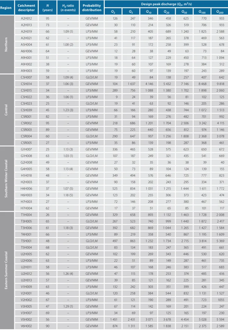
Table 3 At-site probabilistic design flood estimation results
Region Catchmentdescriptor (years)N HEratio
(n events) distributionProbability
Design peak discharge (QP, m3/s)
Q2 Q5 Q10 Q20 Q50 Q100 Q200 N or the rn A2H012 95 – GEV/MM 126 247 346 458 625 770 933 A2H013 73 – GEV/MM 30 110 214 326 519 706 933 A2H019 66 1.09 (1) LP3/MM 58 210 405 689 1 240 1 825 2 588 A2H021 62 – LP3/MM 41 117 187 265 378 469 563 A5H004 61 1.08 (2) LP3/MM 23 91 172 258 399 528 678 A6H006 64 – GEV/MM 12 28 38 49 63 73 84 A9H001 51 – LP3/MM 18 64 127 229 450 713 1 094 A9H002 38 – LP3/MM 19 60 107 169 278 384 512 A9H003 59 – LP3/MM 19 60 97 139 197 243 289 Ce nt ra l C5H007 58 1.09 (4) GLO/LM 19 49 84 138 257 407 642 C5H014 37 1.06 (3) GEV/MM 104 1 637 4 146 5 432 7 146 8 468 9 818 C5H015 34 – LP3/MM 289 756 1 088 1 380 1 702 1 898 2 060 C5H022 36 1.06 (1) LP3/MM 9 24 39 56 81 102 125 C5H023 25 – GLO/LM 19 41 63 92 146 205 286 C5H039 45 1.23 (3) LP3/MM 66 166 280 438 744 1 072 1 513 C5R001 82 – LP3/MM 31 94 169 276 482 701 992 C5R002 95 – GEV/MM 218 686 1 201 1 704 2 506 3 242 4 115 C5R003 89 – GEV/MM 75 225 440 656 812 974 1 146 C5R004 60 – GLO/LM 290 647 937 1 256 1 808 2 368 3 078 C5R005 27 – LP3/MM 35 86 139 198 287 368 461 So ut her n W in ter C oa st al G1H007 25 1.13 (3) GEV/MM 336 465 528 575 623 650 672 G1H008 63 1.03 (1) GLO/LM 107 187 249 321 435 541 669 G2H008 49 – GEV/MM 27 32 35 36 38 39 40 G4H005 58 1.13 (4) GEV/MM 50 73 89 104 124 139 155 H1H018 48 – GEV/MM 349 494 576 646 725 777 823 H2H003 37 – GEV/MM 90 158 202 243 295 334 371 H4H006 37 1.07 (5) GEV/MM 525 834 1 031 1 215 1 444 1 611 1 772 H6H003 34 1.18 (5) GEV/MM 123 202 255 306 373 423 474 H7H003 27 – LP3/MM 72 146 208 277 380 467 562 H7H004 62 – GEV/MM 17 37 51 65 85 101 117 Ea st er n S um m er C oa st al T1H004 26 – GEV/MM 329 658 893 1 132 1 463 1 728 2 008 T3H005 65 – GLO/LM 267 523 740 999 1 440 1 872 2 417 T3H006 61 1.18 (3) GEV/MM 392 682 869 1 044 1 265 1 427 1 584 T4H001 66 – LP3/MM 89 219 358 540 867 1 195 1 609 T5H001 48 – GLO/LM 497 863 1 232 1 734 2 715 3 814 5 369 T5H004 68 – GLO/LM 83 134 183 247 365 491 661 U2H005 62 – GEV/MM 102 199 269 343 446 530 620 U2H006 63 – LP3/MM 22 51 89 149 287 461 735 U2H011 58 – LP3/MM 46 107 168 246 383 517 683 U2H012 56 1.26 (4) GEV/MM 47 115 178 253 374 485 616 U2H013 57 – GEV/MM 39 85 121 162 225 281 345 V1H009 63 – LP3/MM 132 242 303 351 399 426 447 V2H001 46 – GLO/LM 120 258 384 544 832 1 131 1 527 V2H002 67 – LP3/MM 61 121 190 289 491 723 1055 V3H005 47 1.29 (1) GEV/MM 67 114 142 169 201 224 247 V3H007 69 – LP3/MM 34 69 97 125 165 197 230 V5H002 56 – GEV/MM 1 451 2 431 3 071 3 678 4 454 5 028 5 594 V6H002 90 – GEV/MM 874 1 311 1 585 1 838 2 151 2 375 2 589
input to the SDF method (Equation 6; Alexander 2002) to ultimately estimate the deterministic design floods.
QT1, 2 = 0.278 C2 100 + ⎛⎜⎝ YT 2.33⎛⎜⎝⎛⎜⎝ C100 100 – C2 100⎛⎜⎝ IT1,2A (6) Where:
QT1 = design peak discharge (m3/s)
estimated using the standard SDF method
QT2 = design peak discharge (m3/s)
estimated using the new SDF procedure
A = catchment area (km²)
C2 = 2-year return period runoff
coefficient
C100 = 100-year return period runoff
coefficient
IT1 = average areal design rainfall
intensity (mm/h) estimated using Equations 2, 4 and Equation 5
IT2 = average areal design rainfall
intensity (mm/h) estimated using Equations 3, 5 and the RLMA&SI approach
YT = return period factor
RESULTS AND DISCUSSION
The results from the application of the above methodology in the 48 catchments are presented in this section.At-site probabilistic flood
frequency analyses
The at-site probabilistic design flood
estimation results (QP) are presented in
Table 3.
The average AMS record length of all the catchments listed in Table 3 is 56 years, while only 40 events (1.5%) of the 2 665 AMS events were being subjected to the
HE extrapolations, as discussed in the
Methodology section above. The statistical properties of each AMS dataset also con-firmed the asymmetrical nature thereof, i.e. a high degree of variability and skewness. Consequently, the GEV/MM and LP3/MM probability distributions were regarded as the most suitable distributions in 46% and 38% of all the catchments, respectively. The GLO/LM probability distribution proved to be the most appropriate distribution in only 16% of all the catchments. The proba-bilistic plots based on the ranked AMS and Cunnane plotting position (Equation 1) at
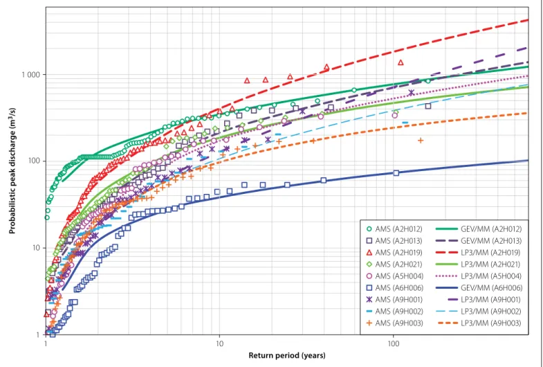
a catchment level in the four climatological regions are shown in Figures 2 to 5(b).
It is evident from Figures 2 to 5(b) that the dispersion about the mean (standard deviation) is relatively high in most of the catchments, while, due to the asymmetrical nature of each AMS, the lower tails of the probability distribution curves proved to be generally longer than the upper tails. At a regional level, the probabilistic curve fitting was dominated by LP3/MM distribution in the NR (Figure 2) and CR (Figure 3), while the GEV/MM distribution was the most appropriate in both the SWCR (Figure 4) and ESCR (Figures 5(a) and (b)). The use of the GLO/LM distribution was limited to the CR (three catchments), ESCR (four catchments), and SWCR (one catchment). Overall, the above selection and use of theoretical probability distributions also proved to be in agreement with the general recommendations for at-site probabilistic flood frequency analyses in South Africa. For example, Alexander (2001) recommends only the LP3 distribution, Görgens (2007) recommends both the LP3 and GEV distribu-tions, while Van der Spuy and Rademeyer (2016) extend their recommendation by
Pr ob ab ilis tic p eak d is char ge (m 3/s ) 1 000 100 10 1 100 10 1
Return period (years)
AMS (A2H012) GEV/MM (A2H012) AMS (A2H013) AMS (A2H019) AMS (A2H021) AMS (A5H004) AMS (A6H006) AMS (A9H001) AMS (A9H002) AMS (A9H003) GEV/MM (A2H013) LP3/MM (A2H019) LP3/MM (A2H021) LP3/MM (A5H004) GEV/MM (A6H006) LP3/MM (A9H001) LP3/MM (A9H002) LP3/MM (A9H003)
Figure 2 Probabilistic plots (1 ≤ T ≤ 1 000-year) based on the ranked AMS and Cunnane plotting position (Equation 1) at a catchment level in the Northern Region
Figure 4 Probabilistic plots (1 ≤ T ≤ 1 000-year) based on the ranked AMS and Cunnane plotting position (Equation 1) at a catchment level in the SWC Region Pr ob ab ilis tic p eak d is char ge (m 3/s ) 1 000 100 10 1 100 10 1
Return period (years)
AMS (G1H007) GEV/MM (G1H007) AMS (G1H008) AMS (G2H008) AMS (G4H005) AMS (H1H018) AMS (H2H003) AMS (H4H006) AMS (H6H003) AMS (H7H003) GLO/LM (G1H008) GEV/MM (G2H008) GEV/MM (G4H005) GEV/MM (H1H018) GEV/MM (H2H003) GEV/MM (H4H006) GEV/MM (H6H003) LP3/MM (H7H003) AMS (H7H004) GEV/MM (H7H004)
Figure 3 Probabilistic plots (1 ≤ T ≤ 1 000-year) based on the ranked AMS and Cunnane plotting position (Equation 1) at a catchment level in the Central Region Pr ob ab ilis tic p eak d is char ge (m 3/s ) 1 000 100 10 1 100 10 1
Return period (years)
10 000 AMS (C5H007) GLO/LM (C5H007) AMS (C5H014) AMS (C5H015) AMS (C5H022) AMS (C5H023) AMS (C5H039) AMS (C5R001) AMS (C5R002) AMS (C5R003) AMS (C5R005) AMS (C5R004) LP3/MM (C5H015) GEV/MM (C5H014) LP3/MM (C5H022) GLO/LM (C5H023) LP3/MM (C5H039) LP3/MM (C5R001) GEV/MM (C5R002) GEV/MM (C5R003) GLO/LM (C5R004) LP3/MM (C5R005)
Figure 5(a) Probabilistic plots (1 ≤ T ≤ 1 000-year) based on the ranked AMS and Cunnane plotting position (Equation 1) at a catchment level in the ESC Region Pr ob ab ilis tic p eak d is char ge (m 3/s ) 10 000 1 000 100 10 1 100 10 1
Return period (years)
AMS (T1H004) AMS (T3H005) AMS (T3H006) AMS (T4H001) AMS (T5H001) AMS (T5H004) AMS (U2H005) AMS (U2H006) AMS (U2H011) GEV/MM (T1H004) GLO/LM (T3H005) GEV/MM (T3H006) LP3/MM (T4H001) GLO/LM (T5H001) GLO/LM (T5H004) GEV/MM (U2H005) LP3/MM (U2H006) LP3/MM (U2H011)
Figure 5(b) Probabilistic plots (1 ≤ T ≤ 1 000-year) based on the ranked AMS and Cunnane plotting position (Equation 1) at a catchment level in the ESC Region Pr ob ab ilis tic p eak d is char ge (m 3/s ) 10 000 1 000 100 10 1 100 10 1
Return period (years)
AMS (T1H004) AMS (T3H005) AMS (T3H006) AMS (T4H001) AMS (T5H001) AMS (T5H004) AMS (U2H005) AMS (U2H006) AMS (U2H011) GEV/MM (T1H004) GLO/LM (T3H005) GEV/MM (T3H006) LP3/MM (T4H001) GLO/LM (T5H001) GLO/LM (T5H004) GEV/MM (U2H005) LP3/MM (U2H006) LP3/MM (U2H011)
including the LN distribution as well. The GLO/LM probability distribution is used extensively internationally as a standard procedure for flood frequency analysis, while LM parameter estimators could be used for the screening of discordant data and test-ing clusters for homogeneity (Smithers & Schulze 2000a). However, Alexander (2001) cautioned that LM parameter estimators are too robust against outliers, and emphasised that both low and high outliers are important characteristics of the flood peak maxima. The suppression of the effect of outliers could result in unrealistic estimates of higher return period values.
Estimation of catchment
response time
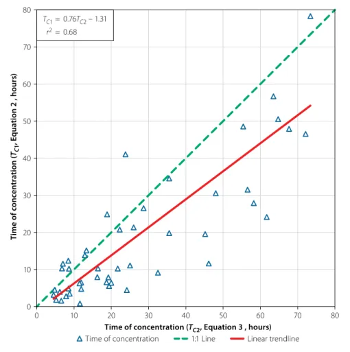
A scatter plot of the catchment response times estimated using Equation 2 (USBR) and Equation 3 (G&S) is shown in Figure 6.
As shown in Figure 6, the r² value of 0.68 confirms the moderate degree of association between the catchment response times esti-mated using Equations 2 and 3, respectively. The USBR method’s (Equation 2) slope (0.76), less than unity and negative y-inter-cept (-1.31), highlight that this method has
an overall tendency to underestimate the TC
values in comparison to the G&S method (Equation 3). On average, Equation 2 under-estimated the time of concentration with 46% in 38 catchments when compared to Equation 3, while an average overestima-tion of 36% is evident in the 10 remaining catchments. Such average differences in the catchment response time must be clearly understood in the context of the actual response time associated with the size of a particular catchment, as the impact thereof might be critical in a small catchment, while being less significant in a larger catchment. However, irrespective of the catchment size and/or differences in response time,
these estimated TC values will have a direct
impact on both the estimates of design rainfall and peak discharge, all of which are elaborated on in the subsequent sections.
Estimation of design rainfall
A scatter plot of the design rainfall depths
(PT1 and PT2) associated with the TC1 and
TC2 values in each catchment are shown in
Figure 7.
It is evident from Figure 7 that the degree of association between the two DDF approaches decreases with an increasing return period, with the r² values rang-ing between 0.34 (T = 2-year) and 0.25 (T = 200-year). The modified Hershfield/
Ti m e o f c on ce nt ra ti on ( TC1 , E qu at io n 2 , h ou rs ) 80 70 60 50 40 30 20 10 0
Time of concentration (TC2, Equation 3 , hours)
80 70 60 50 40 30 20 10 0
Figure 6 Scatter plot of the TC1 (Equation 2) and TC2 (Equation 3) values at a catchment level TC1 = 0.76TC2 – 1.31
r2 = 0.68
1:1 Line Linear trendline Time of concentration
Figure 7 Scatter plot of the modified Hershfield/TR102 and RLMA&SI design rainfall depths at a catchment level H er sh fi eld /T R1 02 des ig n r ai nfa ll ( PT1 , E qu at io n 4 , m m ) 350 300 250 200 150 100 50 0 350 300 250 200 150 100 50 0
RLMA&SI design rainfall (PT2, mm) 1:2-year (r2 =0.34) 1:5-year (r2 =0.34) 1:10-year (r2 =0.33) 1:20-year (r2 =0.31) 1:50-year (r2 =0.29) 1:100-year (r2 =0.27) 1:200-year (r2 =0.25)
Table 4 Deterministic design flood estimation results
Region Catchmentdescriptor Standard SDF method (Equation 6; QT1, m
3/s) New SDF procedure (Equation 6; Q T2, m3/s) Q2 Q5 Q10 Q20 Q50 Q100 Q200 Q2 Q5 Q10 Q20 Q50 Q100 Q200 N or the rn A2H012 218 728 1 193 1 719 2 522 3 214 3 962 271 774 1 183 1630 2 305 2 892 3 543 A2H013 94 307 499 717 1 053 1 346 1 666 144 408 615 837 1 158 1 427 1 716 A2H019 294 875 1 379 1 949 2 874 3 729 4 691 375 1 065 1 615 2 209 3 088 3 836 4 652 A2H021 245 752 1 201 1 721 2 561 3 336 4 241 167 475 721 987 1 384 1 724 2 095 A5H004 28 125 214 315 473 611 761 49 185 294 412 587 735 894 A6H006 20 93 163 243 364 466 575 18 70 111 156 222 277 338 A9H001 37 205 360 542 831 1 089 1 383 57 284 466 661 943 1 174 1 420 A9H002 10 61 110 167 252 325 402 18 88 146 210 307 391 482 A9H003 9 52 93 141 213 275 340 11 57 93 132 188 234 283 Ce nt ra l C5H007 45 150 245 354 519 662 812 67 188 282 381 523 640 762 C5H014 674 2 072 3 304 4 769 7 114 9 278 11 746 828 2 352 3 536 4 781 6 562 8 038 9 575 C5H015 242 726 1 154 1 646 2 435 3 172 4 001 396 1 115 1 672 2 261 3 109 3 815 4 556 C5H022 24 85 141 205 300 380 465 11 31 46 63 88 109 131 C5H023 36 126 209 304 445 563 689 27 77 115 156 217 267 321 C5H039 234 704 1 125 1 605 2 383 3 105 3 935 215 605 907 1 226 1 686 2 069 2 470 C5R001 66 199 313 448 656 851 1 054 68 192 290 395 552 685 830 C5R002 351 1 059 1 692 2 418 3 591 4 679 5 931 324 922 1 398 1 907 2 658 3 290 3 975 C5R003 90 291 471 678 993 1 273 1 567 111 312 469 637 881 1 088 1 307 C5R004 236 710 1 135 1 620 2 404 3 132 3 969 221 621 937 1 275 1 775 2 200 2 661 C5R005 38 132 220 320 468 593 726 27 77 116 159 223 278 339 So ut her n W in ter C oa st al G1H007 149 298 421 555 752 912 1 086 135 242 321 402 514 604 700 G1H008 136 312 464 631 872 1 069 1 275 172 301 392 481 600 691 782 G2H008 28 64 95 129 178 218 261 18 34 45 57 74 88 103 G4H005 59 136 202 274 379 465 554 38 70 95 120 155 183 214 H1H018 64 147 219 297 411 504 601 96 171 226 281 358 420 485 H2H003 188 410 600 806 1 105 1 352 1 611 154 277 367 457 582 681 784 H4H006 498 916 1 252 1 607 2 130 2 580 3 066 369 657 866 1 079 1 373 1 609 1 853 H6H003 142 321 475 643 886 1 085 1 294 160 289 386 485 623 735 852 H7H003 121 264 386 518 711 869 1 036 89 178 251 331 455 564 686 H7H004 24 55 83 112 155 190 227 15 30 42 55 76 94 114 Ea st er n S um m er C oa st al T1H004 227 1 069 1 745 2 486 3 644 4 647 5 765 138 673 1 108 1 583 2 299 2 922 3 612 T3H005 137 644 1 051 1 500 2 202 2 807 3 487 100 477 780 1 107 1 598 2 020 2 478 T3H006 186 876 1 429 2 032 2 975 3 794 4 702 147 703 1 152 1 641 2 379 3 021 3 724 T4H001 133 555 949 1 409 2 121 2 750 3 450 92 334 539 772 1 145 1 491 1 891 T5H001 168 768 1 238 1 739 2 503 3 150 3 884 122 585 970 1 405 2 094 2 721 3 443 T5H004 53 291 507 752 1 122 1 436 1 776 27 127 207 293 422 531 649 U2H005 132 599 963 1 348 1 937 2 433 2 997 71 353 594 868 1 304 1 707 2 172 U2H006 40 226 399 596 895 1 148 1 421 20 97 162 238 359 473 605 U2H011 33 193 348 526 795 1 024 1 268 18 88 146 212 318 414 526 U2H012 46 255 447 664 994 1 274 1 576 31 156 266 393 601 800 1 033 U2H013 47 278 498 752 1 136 1 462 1 811 21 103 169 240 347 440 541 V1H009 41 126 204 292 422 531 647 45 110 161 215 294 360 433 V2H001 145 367 553 760 1 086 1 381 1 712 99 245 362 488 681 848 1 033 V2H002 95 249 380 526 755 960 1 187 72 178 264 358 503 629 771 V3H005 69 178 271 375 537 683 846 66 160 231 306 413 501 593 V3H007 34 106 171 245 354 446 542 29 70 102 135 183 222 264 V5H002 927 2 379 3 553 4 899 6 908 8 715 10 749 904 2 248 3 295 4 406 6 019 7 376 8 839 V6H002 560 1 429 2 150 2 960 4 194 5 306 6 563 477 1 176 1 714 2 278 3 080 3 741 4 443
TR102 design rainfall depths were generally lower than the RLMA&SI design rainfall depths for T ≤ 20-year. The frequency of these underestimations decreased with an increase in return period (e.g. 85% of the events at T = 2-year versus 50% of the events at T = 20-year), while the magni-tude thereof remained relatively constant and varied between –21% and –25%. For T > 20-year, the opposite trend is evident. The modified Hershfield/TR102 design rainfall depths were generally higher than the RLMA&SI design rainfall depths, while the frequency of these overestimations increased with an increase in return period (e.g. 50% of the events at T = 20-year versus 61% of the events at T = 200-year). The latter overestimations remained relatively constant and varied between 11% and 19%.
The above differences, evident between the two DDF approaches, are most likely attributed to: (i) the longer record lengths and stringent data quality control proce-dures used in the RLMA&SI approach, and (ii) the different approaches to design rainfall estimation used, i.e. a single site approach (Adamson 1981) versus a regional approach (Smithers & Schulze 2003; 2004). Furthermore, inconsistencies between the
estimated 24-hour event values estimated using Equation 4 (modified Hershfield equation) and the TR102 1-day design rainfall information, on which the equation is based, were also evident. According to Smithers and Schulze (2003), the latter inconsistencies are ascribed to the fact that the functional relationship of Equation 4 does not accommodate the curvilinear relationship between design rainfall depth and log-transformed duration as applicable to most rainfall stations.
The above differences in design rain-fall depths using the two different DDF approaches are truly appreciated when converted into design rainfall intensities, i.e. underestimated time parameters would result in higher design rainfall intensities, while the overestimation of time parameters is associated with lower design rainfall intensities. Both these scenarios would have a direct impact on the estimation of design floods, as detailed in the next section.
Estimation of deterministic
design floods
The SDF design flood estimation results
(Equation 6; QT1and QT2) are presented
in Table 4, while the peak discharge ratios
estimated using Equation 7 are shown in Figures 8(a) to 8(e).
QT-ratio = ⎛⎜⎝ QT1,2 QP ⎛ ⎜ ⎝ – 1 (7) Where:
QT-ratio = peak discharge ratio (positive = overestimation and negative = underestimation)
QT1 = design peak discharge (m3/s)
estimated using the standard SDF method
QT2 = design peak discharge (m3/s)
estimated using the new SDF procedure
QP = at-site probabilistic design peak
discharge (m3/s)
A summary of the goodness-of-fit (GOF) statistics based on the comparison between the at-site probabilistic design floods
(QP; Table 3) and the SDF design floods
(Table 4) is listed in Table 5. The root mean square error (RMSE) is specifically included in Table 5 to ensure that the accumulated over- and/or underestima-tions are accounted for, i.e. to highlight the actual size (not source or type) of errors
Figure 8(a) Peak discharge ratios (Equation 7) at a catchment level in the Northern Region; light fill = standard SDF method (QT1) and dark fill = new SDF procedure (QT2) Pe ak d is char ge ra tio (E qu at io n 7 ) 6.5 6.0 5.5 5.0 4.5 4.0 3.5 3.0 2.5 2.0 1.5 1.0 0.5 0 Region –0.5 –1.0
A2H012 A2H013 A2H019 A2H021 A5H004 A6H006 A9H001 A9H002 A9H003
200-year 100-year 50-year 20-year 10-year 5-year 2-year 200-year 100-year 50-year 20-year 10-year 5-year 2-year
Figure 8(b) Peak discharge ratios (Equation 7) at a catchment level in the Central Region; light fill = standard SDF method (QT1) and dark fill = new SDF procedure (QT2) Pe ak d is char ge ra tio (E qu at io n 7 ) 3.5 3.0 2.5 2.0 1.5 1.0 0.5 0 Region –0.5 C5H007 C5H014 C5H015 C5H022 C5H023 C5H039 C5R001 C5R002 C5R003 200-year 100-year 50-year 20-year 10-year 5-year 2-year 200-year 100-year 50-year 20-year 10-year 5-year 2-year SDF Basin 9 C5R004 C5R005
Figure 8(c) Peak discharge ratios (Equation 7) at a catchment level in the SWC Region; light fill = standard SDF method (QT1) and dark fill = new SDF procedure (QT2) Pe ak d is char ge ra tio (E qu at io n 7 ) 5.5 5.0 4.5 4.0 3.5 3.0 2.5 2.0 1.5 1.0 0.5 0 Region –0.5 –1.0 G1H007 G1H008 G2H008 G4H005 H1H018 H2H003 H4H006 H6H003 H7H003 200-year 100-year 50-year 20-year 10-year 5-year 2-year 200-year 100-year 50-year 20-year 10-year 5-year 2-year SDF Basin 17 SDF Basin 18 H7H004
Figure 8(e) Peak discharge ratios (Equation 7) at a catchment level in the ESC Region; light fill = standard SDF method (QT1) and dark fill = new SDF procedure (QT2) Pe ak d is char ge ra tio (E qu at io n 7 ) 4.5 4.0 3.5 3.0 2.5 2.0 1.5 1.0 0.5 0 Region –0.5 –1.0 U2H012 U2H013 V1H009 V2H001 V2H002 V3H005 V3H007 V5H002 V6H002 200-year 100-year 50-year 20-year 10-year 5-year 2-year 200-year 100-year 50-year 20-year 10-year 5-year 2-year SDF Basin 25 SDF Basin 26
Figure 8(d) Peak discharge ratios (Equation 7) at a catchment level in the ESC Region; light fill = standard SDF method (QT1) and dark fill = new SDF procedure (QT2) Pe ak d is char ge ra tio (E qu at io n 7 ) 4.0 3.5 3.0 2.5 2.0 1.5 1.0 0.5 0 Region –0.5 –1.0
T1H004 T3H005 T3H006 T4H001 T5H001 T5H004 U2H005 U2H006 U2H011
200-year 100-year 50-year 20-year 10-year 5-year 2-year 200-year 100-year 50-year 20-year 10-year 5-year 2-year
produced by the two SDF procedures, with the objective function to minimise the RMSE to zero.
The results contained in Tables 4 and 5, as well as Figures 8(a) to 8(e), are indicative of several trends associated with specific catchments and return periods, which are highlighted below:
■ Northern Region (SDF basins 1–3,
Figure 8(a)): The SDF flood peaks (QT1
and QT2) exceeded the at-site
probabi-listic flood peaks (QP) in all the
catch-ments, except for catchments A9H002 and A9H003 in SDF basin 3. In 56% of all the catchments considered, the new SDF
procedure (QT2, Equation 6) resulted
in improved estimates in comparison
to the standard SDF method (QT1,
Equation 6) when compared to the at-site probabilistic flood estimates, especially in catchments A2H021 and A6H006. In the latter catchments, the standard SDF
method (QT1, Equation 6) overestimated
the at-site probabilistic flood peaks with between 62% and 653%, whereas the new SDF procedure’s overestimations are limited to 300%. On average, the new
SDF procedure (QT2, Equation 6)
demon-strated the best results, especially for the higher return periods (e.g. T = 10–200-year; 142%–175% overestimation, ≤ 5% underestimation, 0.72 ≤ r² ≤ 0.93, and 1 658 ≤ RMSE ≤ 3 775).
■ Central Region (SDF basin 9,
Figure 8(b)): The standard SDF flood
peaks (QT1) exceeded the at-site
probabilistic flood peaks (QP) in all the
catchments, except for the lower return periods (T ≤ 20-year) in catchments C5H014 and C5R004. In more than 80% of all the catchments considered, the
new SDF procedure (QT2, Equation 6)
resulted in improved estimates in com-parison to the standard SDF method
(QT1, Equation 6) when compared to the
at-site probabilistic flood estimates. The
standard SDF method (QT1, Equation 6)
overestimated the at-site probabilistic flood peaks with between 3% and 323%, whereas the new SDF procedure’s overestimations are limited to 264%. However, in catchment C5H014, both the standard SDF method and new SDF procedure overestimated the at-site probabilistic flood peaks by a factor > 5 for T = 2-year. For all other return
periods, the new SDF procedure (QT2,
Equation 6) demonstrated the best aver-age results (39%–165% overestimation, ≤ 12% underestimation, 0.92 ≤ r² ≤ 0.95, and 963 ≤ RMSE ≤ 2 735).
■ Southern Winter Coastal Region (SDF
basins 17 and 18, Figure 8(c)): The
new SDF procedure (QT2, Equation 6)
resulted in improved estimates in com-parison to the standard SDF method
(QT1, Equation 6) when compared to the
at-site probabilistic flood estimates in all the catchments, except in catchment G1H007 where both methods had a tendency to underestimate the at-site probabilistic flood peaks with between 20% and 60%. In all other catchments and corresponding return periods, the
new SDF procedure (QT2, Equation 6)
demonstrated the best average results (41%–64% overestimation, 15%–39% underestimation, 0.58 ≤ r² ≤ 0.84, and 373 ≤ RMSE ≤ 686).
■ Eastern Summer Coastal Region (SDF
basins 23–26, Figures 8(d)–8(e)): The
new SDF procedure (QT2, Equation 6)
resulted in improved estimates in com-parison to the standard SDF method
(QT1, Equation 6) when compared to
the at-site probabilistic flood estimates in all the catchments, except for the two-year return period. The new SDF
procedure (QT2, Equation 6)
demon-strated better average results (11%–81% overestimation, 18%–43% underestima-tion, 0.71 ≤ r² ≤ 0.98, and 443 ≤ RMSE ≤ 5 293) than the standard SDF method, i.e. 37%–150% overestimation, 8%–37% underestimation, 0.63 ≤ r² ≤ 0.95, and 752 ≤ RMSE ≤ 9 180.
Overall, the new SDF procedure (QT2,
Equation 6) resulted in improved estimates in comparison to the standard SDF method
Table 5 Average QT-ratios(Equation 7) and GOF statistics at a regional level
Region GOF Standard SDF method (Equation 7) New SDF procedure (Equation 7)
Q2 Q5 Q10 Q20 Q50 Q100 Q200 Q2 Q5 Q10 Q20 Q50 Q100 Q200 NR QT-ratio (+) 1.96 2.17 2.12 2.11 2.14 2.18 2.22 2.45 2.31 1.97 1.75 1.53 1.42 1.54 QT-ratio (–) –0.50 –0.13 –0.04 –0.01 –0.09 –0.15 –0.22 –0.24 –0.05 –0.04 –0.05 –0.05 –0.04 –0.04 r² value 0.48 0.74 0.73 0.67 0.56 0.49 0.43 0.55 0.85 0.93 0.93 0.86 0.79 0.72 RMSE 332 1 068 1 688 2 364 3 400 4 305 5 292 390 1 134 1 658 2 166 2 821 3 307 3 775 CR QT-ratio (+) 1.55 1.27 1.21 1.14 1.04 0.88 0.81 1.65 1.03 0.89 0.70 0.50 0.43 0.39 QT-ratio (–) –0.17 –0.04 –0.20 –0.12 – – – –0.23 –0.07 –0.10 –0.12 –0.11 –0.10 –0.12 r² value 0.21 0.92 0.91 0.93 0.94 0.95 0.96 0.22 0.95 0.94 0.94 0.93 0.93 0.92 RMSE 615 812 1 339 1 635 2 250 3 081 4 244 760 963 1 097 1 393 1 822 2 228 2 735 SWC R QT-ratio (+) 0.40 0.76 1.05 1.31 1.47 1.69 1.91 0.46 0.41 0.41 0.48 0.57 0.64 0.54 QT-ratio (–) –0.48 –0.53 –0.41 –0.29 –0.43 –0.35 –0.27 –0.39 –0.32 –0.33 –0.28 –0.21 –0.15 –0.22 r² value 0.54 0.60 0.63 0.66 0.69 0.72 0.74 0.58 0.66 0.71 0.75 0.79 0.82 0.84 RMSE 361 517 700 949 1 376 1 773 2 218 373 470 509 537 575 619 686 ES CR QT-ratio (+) 0.37 1.08 1.23 1.35 1.43 1.47 1.50 0.11 0.37 0.39 0.46 0.52 0.62 0.81 QT-ratio (–) –0.37 –0.20 –0.33 –0.17 –0.08 –0.17 –0.28 –0.43 –0.18 –0.22 –0.20 –0.21 –0.20 –0.20 r² value 0.95 0.94 0.92 0.90 0.84 0.76 0.63 0.94 0.98 0.97 0.95 0.90 0.82 0.71 RMSE 752 828 1750 2 965 4 991 6 908 9 180 858 443 672 1 347 2 576 3 788 5 293
(QT1, Equation 6) when compared to the at-site probabilistic flood estimates in more than 80% of all the catchments in the four climatological regions. Such improvements in design flood estimation also confirm that catchment response time and design rainfall are fundamental inputs to design flood estimation in ungauged catchments. However, despite the improvement in design flood estimation achieved in this study, the high over- and/or underestimations are still regarded as unacceptable and indicative that neither design rainfall nor catchment response time in these catchments could be regarded as the only fundamental input to design flood estimation. In essence, catch-ment response time should be regarded as enigmatic, since, although it is assumed to be an independent time parameter, it is actually dependent on the peak discharge, which in turn is also dependent on the design rainfall. Therefore, the latter over- and/or underestimations could also be ascribed to the regional SDF runoff coef-ficients not being representative of the aver-age catchment conditions and/or physical regional descriptors.
The term ‘runoff coefficient’ is com-monly used in flood hydrology (Young et al 2009; SANRAL 2013; Van der Spuy & Rademeyer 2016) to represent the percent-age of effective rainfall that is transformed to direct runoff. Runoff coefficients vary substantially with the time scale of aggre-gation, i.e. in small catchments (< 15 km²) runoff coefficients represent an overall cut-off threshold separating effective rainfall from total rainfall and are readily obtain-able from lookup tobtain-ables, whereas in larger rural catchments, the runoff coefficients are normally associated with land use, soils and catchment slopes (Efstratiadis et al 2014). In both cases, these runoff coef-ficients are regarded as constant; however, it is obvious that its value depends both on the antecedent soil moisture conditions and on the rainfall intensity. To overcome this shortcoming, larger runoff coefficients are normally assigned to higher return periods, i.e. runoff coefficients increase as the return period increases, but such recom mendations are not based on sys-tematic investigations and favour arbitrary choices (Efstratiadis et al 2014).
Despite the simplicity of estimating runoff coefficients, it is evident that runoff coefficients play a secondary role in the overall predictive capacity of most deter-ministic design flood estimation methods in ungauged catchments. Hence, several
modifications, e.g. modified runoff coef-ficients (Pegram 2003) and probabilistic approaches (Alexander 2002; Calitz & Smithers 2016), were suggested locally and abroad (Pilgrim & Cordery 1993) to deviate from a deterministic to a more probabilis-tic-deterministic approach. The SDF meth-od is a typical example thereof, but due to several design limitations – i.e. region-alisation scheme adopted, lack of testing for homogeneity, outdated design rainfall information (TR102), etc – the method generally proved to be too conservative (Gericke & Du Plessis 2012). However, by using the more appropriate design rainfall information and catchment response times as input to the SDF method (this study), the results improved accordingly. In doing so, the variation of runoff coefficients with return period is also incorporated. Thus, as the intensity and volume of rainfall increases, the effect of the internal storage of catchments decreases, which leads to an increase in the runoff coefficients.
Typically, the large proportional
dif-ferences between the C2 and C100 runoff
coefficients (Equation 6), highlight that the SDF method assumes that a larger propor-tion of rainfall would contribute to the flood peaks and acknowledge that the ante-cedent soil moisture status of a catchment introduces additional variability into the rainfall-runoff process. However, variability increases with an increase in catchment size; hence, the difficulty to successfully establish a relationship between regional/ catchment descriptors and runoff coef-ficients in larger catchments. Hydrological literature, e.g. Pilgrim and Cordery (1993), Parak and Pegram (2006), and Gericke and Du Plessis (2012) also confirmed the latter and concluded that runoff coefficients are essentially functions of the return period and catchment response time.
CONCLUSIONS
The overall objective of this study was to independently test and compare the latest catchment response time and design rain-fall estimation methodologies with current well-known and simplified methodolo-gies used in South Africa to ultimately highlight the impact thereof on design flood estimation.
Building upon the critical assessment of available definitions, estimation procedures and the results from this study, it is evident that catchment response time, design rainfall, and to some lesser extent runoff
coefficients, are key input parameters for design flood estimation in ungauged catch-ments, and have a significant impact on the design of hydraulic structures. Typically, high runoff coefficients, underestimated time parameters and associated lower design rainfall depths, although of much higher intensities, would result in over-designed hydraulic structures, while low runoff coefficients and overestimated time
parameterswould result in underdesigns.
Not only will hydraulic structures be over- or under designed, but associated socio-economic implications might render some projects as not being feasible, while any loss of life due to excessive flood damages and insufficient infrastructure is not excluded. It is recommended that the current well-known and simplified catchment response
time (USBR TC equation) and design rainfall
(modified Hershfield/TR102 DDF approach) estimation methodologies should be
replaced with the empirical G&S TC
equa-tions and the RLMA&SI DDF approach when deterministic design floods are estimated in ungauged catchments in South
Africa. However, since the G&S TC
equa-tions (Equation 3) are limited to only four climatological regions in South Africa, the further refinement thereof in terms of cali-bration, verification and possible regionali-sation in other regions, is acknowledged. The proposed new SDF procedures are recommended for the estimation of flood peaks with return periods in excess of and including 10 years (T ≥10 years). In order to improve the depth of hydrological runoff data in South Africa, it is recommended that flow records be obtained from the DWS and verified. The verified data can then be utilised to improve on the findings in this study and to refine methods to be used for the purpose of design flood estimations, including those for T < 10 years.
Furthermore, the current research ini-tiative of Calitz and Smithers (2016), which focuses on the development and assess-ment of regional runoff coefficients to be incorporated in the Probabilistic Rational Method (PRM) for South Africa, should be supported and welcomed by all research academic institutions and engineering practitioners involved in modern flood hydrology practice.
ACKNOWLEDGEMENTS
Support for this research by the National Research Foundation (NRF), University of KwaZulu-Natal (UKZN) and Central