NBER WORKING PAPER SERIES
SIMULATING THE RESPONSE TO REFORM OF CANADA’S INCOME SECURITY PROGRAMS
Michael Baker Jonathan Gruber
Kevin Milligan Working Paper9455
http://www.nber.org/papers/w9455
NATIONAL BUREAU OF ECONOMIC RESEARCH 1050 Massachusetts Avenue
Cambridge, MA 02138 January 2003
This paper was prepared as part of the NBER Aging Program’s International Social Security project. We thank participants at the International Social Security conference in Assmannshausen Germany in May, 2002 for helpful comments. The views expressed herein are those of the authors and not necessarily those of the National Bureau of Economic Research.
©2003 by Michael Baker, Jonathan Gruber, and Kevin Milligan. All rights reserved. Short sections of text not to exceed two paragraphs, may be quoted without explicit permission provided that full credit including notice, is given to the source.
Simulating the Response to Reform of Canada’s Income Security Programs Michael Baker, Jonathan Gruber, and Kevin Milligan
NBER Working Paper No. 9455 January 2003
JEL No. H0
ABSTRACT
We explore the fiscal implications of reforms to the Canadian retirement income system by decomposing the fiscal effect of reforms into two components. The mechanical effect captures the change in the government's budget assuming no behavioral response to the reform. The second component is the fiscal implication of the behavioral effect, which captures the influence of any induced changes in elderly labor supply on government budgets. We find that the behavioral response can account for up to half of the total impact of reform on government budgets. The behavioral response affects government budgets not only in the retirement income system but also through increased income, payroll, and consumption tax revenue on any induced labor market earnings among the elderly. We show that fully accounting for the behavioral response to reforms can change the cost estimates and distributive impact of retirement income reforms.
Michael Baker Jonathan Gruber Kevin Milligan
Department of Economics Department of Economics Department of Econmics University of Toronto MIT, E52-355 University of British Columbia 150 St. George Street 50 Memorial Drive #997-1873 East Mall
Toronto, Ontario M5S 3G7 Cambridge, MA 02142 Vancouver, B.C.
Canada and NBER Canada V6T1Z1
and NBER [email protected] and NBER
1.0 Introduction
Expenditures on public pensions in Canada are projected to be over C$54 billion in 2002-2003. The extensive income security system in Canada, which consists of a demogrant, work-related pensions, and income-tested transfers, provides an important source of income for older Canadians. However, the system has experienced periodic crises when the streams of projected future expenditures and revenues fall out of alignment. The future may offer further turbulence. The elderly dependency ratio in Canada, the ratio of older persons to working age persons, is projected to rise from 0.20 in 2000 to 0.40 in 2050 (Office of the Superintendent of Financial Institutions 1998). As a result, this income security system may face pressure for reform in the years to come.
Any reforms that reduce program generosity will have two types of effects on public sector budgets. The first is a mechanical effect of the reduction. The magnitude of the government’s benefit expenditures and tax receipts will change mechanically with any changes to the programs. The second effect is a dynamic effect through changing retirement behavior. Our past research has shown that the retirement decisions of older Canadians are sensitive to the labor supply incentives in the income security system. This implies that reform to this system can have important indirect effects on fiscal balances through behavioral changes.
In this paper, we explore the fiscal implications of two alternative reforms, and describe how those implications depend on the types of behavioral responses estimated in our previous work. The first reform that we consider is a three year increase in both the age at which individuals are eligible for early retirement benefits, and the normal retirement age for all retirement programs. The second is a move to a common income
security system for all countries in this research project. The Common Reform replaces Canada’s existing mix of demogrants and earnings-related benefits with one large earnings-related benefit, similar in structure to the existing Canada Pension Plan.
Our major findings are that both of these reforms would have enormous impacts on the fiscal position of the Canadian retirement income system. An increase of three years in the age of benefits eligibility would improve the government’s fiscal position by about one quarter of the base level of benefits, while the second reform raises net
program expenditures by about 50 percent. For both reforms, we find very important behavioral as well as mechanical effects. The first reform significantly reduces the amount of early retirement in Canada, and between 21 and 49 percent of the reduction in program expenditures comes from behavioral responses to this reform. The behavioral response manifests itself in the government budget through lower benefit payments paid to, and more taxes collected from, workers who retire later than under the base system. For the Common Reform, the fiscal implications of behavioral response are also large in magnitude, but smaller relative to the mechanical effect of the increased benefits.
We also document important distributional implications of reform. A delay in retirement ages has somewhat larger negative effects for upper income groups, as they see the largest effective reduction in their benefits. On the other hand, the Common Reform reduces effective benefits for the lowest income groups, by removing the income-tested component of transfers, while at the same time dramatically increasing benefits for upper income groups whose benefits now reflect more fully their higher lifetime earnings.
In the balance of this paper, we first describe in detail the components of Canada’s retirement income system. This is followed by a recounting of the empirical results from our earlier work, upon which the simulations in this paper are based. We then lay out the simulation methodology we employ. Finally, the results are presented along with some concluding remarks.
2.0 Canada’s Retirement Income System
The retirement income system in Canada has three pillars: 1) the Old Age Security Program, 2) the Canada and Quebec Pension Plans and 3) private savings. The first pillar includes the Old Age Security pension (OAS), the Guaranteed Income
Supplement (GIS) and the Allowance. The third pillar includes occupational pensions, as well as other private savings including those accumulated in Registered Retirement Savings Plans (RRSPs), which are a tax subsidized savings vehicle. Our analysis focuses on reforms to the first two pillars of this system, which collectively are referred to as the Income Security (IS) system in Canada. We next provide a brief description of the components of all three pillars, however, to provide the proper context for our results. 2.1 The Old Age Security Program
The Old Age Security program is the oldest pillar of the current retirement system, dating back to 1952. All benefits paid out under the program are financed through general tax revenues rather than past or current contributions. Its principal component is the OAS pension, which is currently payable to anyone aged 65 or older who satisfies a residency requirement.1 The pension is a demogrant, equal to
1
Individuals must have been a Canadian citizen or legal resident of Canada at some point before application, and have resided in Canada for at least 10 years (if currently in Canada) or 20 years (if currently outside Canada). The benefit is prorated for pensioners with less than 40 years of Canadian
$442.66 in March 2002. Individuals who do not meet the residence requirement may be entitled to a partial OAS benefit. Benefits are fully indexed to the Consumer Price Index (CPI), and are fully taxable under the Income Tax Act. There is also an additional “clawback” of benefits from high income beneficiaries. Their benefits are reduced by 15 cents for every dollar of personal net income that exceeds $56,968.
A second component of the OAS program is the GIS. It is an income-tested supplement for OAS pension beneficiaries, which has been in place since 1967. There are separate single and married benefits that in 2002 (January to March) were $526.08 and $342.67 (per person) monthly, respectively. The income test is applied annually based on information from an individual’s (and their partner’s) income tax return. Income for the purpose of testing is the same as for income tax purposes, with the exclusion of OAS pension income. Unlike the OAS clawback the income testing of GIS benefits is based on family income levels. Benefits are reduced at a rate of 50 cents for each dollar of family income, except for couples in which one member is age 65 or older and the other is younger than age 60. For these couples the reduction is 25 cents for each dollar of family income. The GIS is fully indexed to the CPI and is not subject to income taxes at either the federal or provincial level.
The final component of the OAS program is the Allowance, which until recently was called the Spouse’s Allowance.2 This component was introduced in 1975. The
Allowance is an income-tested benefit available to 60-64 year old partners3 of OAS pension recipients and to 60-64 year old widows/widowers. For the partners, the benefit
residence, unless they are “grandfathered” underrules that apply to the persons who were over age 25 and had established attachment to Canada prior to July 1977.
is equal to the OAS pension plus the GIS at the married rate. An income test reduces the OAS pension portion of the Allowance by 75 cents for each dollar of family income until it is reduced to zero, and then the combined GIS benefits of both partners are reduced at 50 cents per dollar of family income. For a widowed partner, the benefit is equal to the OAS pension plus GIS at the widowed rate, and is "taxed-back" equivalently. The Allowance is also fully indexed to the CPI and again is not subject to income taxes at either the federal or provincial level.
2.2 The Canada/Quebec Pension Plan
The second pillar of the retirement system and largest component of the IS system is the Canada Pension Plan (CPP) and Quebec Pension Plan (QPP). These programs, started in 1966, are administered separately by Quebec for the QPP, and the federal government for the CPP.
In contrast to the OAS program, the CPP/QPP are contributory programs. They are financed by payroll taxes on both employers and employees, each at a rate of 4.7 percent (2002). The base for the payroll tax is earnings between the Year's Basic Exemption ($3,500) up to the Year's Maximum Pensionable Earnings (YMPE, $39,100 in 2002). The YMPE approximates average earnings, and is indexed to its growth.
To be eligible for benefits individuals must make contributions in at least one calendar year during the contributory period. The contributory period is defined as the period from attainment of age 18, or January 1, 1966 if later, and normally extended to age 70 or commencement of the retirement pension, whichever is earlier. Starting in 1984 for the QPP and 1987 for the CPP, benefits can be claimed as early as age 60. The
3
The Allowance is available to both spouses and common law partners (same sex or opposite sex) of OAS pension beneficiaries.
“normal retirement age” is 65 and there is an actuarial reduction in benefits of 0.5 percent for each month the initial claim precedes this age, resulting in a maximum 30 percent reduction for claims on the 60th birthday. Symmetrically, benefits are increased by 0.5 for each month the initial claim succeeds age 65 to as late as age 70 (the maximum adjustment is therefore 30 percent). Finally, if an individual claims before age 65 their annual rate of earnings cannot exceed the maximum retirement pension payable at age 65, for the year in which the pension is claimed. This “earnings test” is only applied at the point of application, however. Subsequently, there is no check on the individual's earnings.4
To calculate benefits, an individual’s earnings history is first computed. The earnings history is based on earnings in the contributory period, less any months (a) receiving a disability pension, (b) spent rearing small children,5 (c) between age 65 and the commencement of the pension6, and (d) 15 percent of the remaining months. The last three of these exclusions cannot be used, however, to reduce the contributory period below 120 months after taking into account the offset for months of disability pension receipt. The ratio of each month of earnings in the contributory period to 1/12 of the YMPE for that period is then calculated, with the ratio capped at one. Excess earnings in one month above 1/12 of the YMPE may be applied to months in the same calendar year in which earnings are below 1/12 of the YMPE.
Earnings over the earnings history period are then converted to current dollars in three steps. First the average of the earnings ratios over the contributory period is
4
There are no restrictions on returning to work after the benefit is being paid.
5 This is defined as months where there was a child less than 7 years of age and the worker had zero or
calculated. Second, this average is multiplied by a pension adjustment factor. Until 1998, the pension adjustment factor was the average of the YMPE over the three years prior to (and including) the year of pension receipt. This average was raised to four years for benefits claimed in 1998 and five years for benefits beginning in 1999. Finally, the product of the earnings ratios and the pension adjustment factor is multiplied by 25 percent to arrive at the annual benefit. This benefit can be thought of as a pension that replaces 25 percent of earnings for someone who has average earnings over his or her lifetime. In 2002, the maximum possible monthly retirement benefit works out to $788.75.
While CPP/QPP retirement benefits are based solely on an individual's earnings history,7 survivor pensions are either all or partly based on the earnings history of the
deceased. Partners are eligible for survivor pensions if the deceased made contributions for the lesser of 10 years or one third of the number of years in the contributory period. For survivors under age 65, benefits are equal to a flat rate benefit plus 37.5 percent of the earnings-related pension of the deceased spouse. If the survivor is not disabled or has no dependent children the benefit is reduced by 1/120 for each month s/he is younger than age 45, such that no benefit is payable to individuals aged 35 or younger. Also, benefits to survivors who have dependent children and who are under age 35 only continue as long as the children are dependent.8 For survivors aged 65 and above, the
pension is equal to the greater of a) 37.5 percent of the deceased’s retirement pension
6 Periods after age 65 to age 70 can be substituted for periods prior to age 65 if this will increase their
future retirement pension. 7
Couples do have the option of sharing their benefits for income tax purposes, since taxation is at the individual level. Each spouse can claim up to half of the couple’s total CPP/QPP pension credits. The exact calculation depends on the ratio of their cohabitation period to their joint contributory period.
plus 100 percent of the survivor’s own retirement pension, or b) 60 percent of the
deceased’s retirement pension plus 60 percent of the survivor’s own retirement pension. There is an upper cap on total payments equal to the maximum retirement pension payable in that year.9 Under changes made effective in 1998, however, the rules for maximum payout are changed. The survivor simply receives the larger of their own retirement pension or their survivor pension plus 60 percent of the smaller. Finally, under the CPP children of deceased contributors are also entitled to a (flat rate) benefit if under 18 or a full time student between 18 and 25 (the corresponding QPP benefit ends at age of 18).10
A final dimension of the CPP/QPP is the disability benefit program. The basic benefit is made up of a flat-rate portion, paid to all disabled workers, and an earnings-related portion, which is 75 percent of the applicable CPP/QPP retirement pension, calculated with the contributory period ending at the date of disability. Fewer than 5 percent of older Canadian men are on CPP/ QPP disability. More information can be found in Gruber (2000).
CPP/QPP benefits have been fully indexed to the CPI since 1973. Also, benefits are fully taxable by the federal and provincial governments.
2.3 Private Savings
The third pillar of the retirement income system is the proceeds of private savings. These can take a variety of forms, some of which are explicitly regulated by either federal or provincial governments. For many individuals the most important form is private
9 If the surviving spouse is receiving his or her own CPP disability pension, the sum of the earnings-related
occupational pensions. In 1997, 41.2 percent of paid workers were covered by
occupational pensions, with coverage slightly higher for males than for females (Statistics Canada 1999). Defined benefit pensions are overwhelmingly the most common (86 percent of plan members in 1997) although the recent trend is towards more defined contribution plans.
The other main form of private savings having a public policy dimension is savings in RRSPs. Contributions are deducted from gross earnings in the calculation of taxable income. While in the RRSP, investment earnings on the contributions
accumulate tax-free. There is a yearly limit on contributions that is lower for individuals who participate in an occupational pension plan. Unused contribution room can be carried forward indefinitely. Finally, there are rules covering the start and minimum payout of these savings over the retirement years. More information on RRSPs can be found in Milligan (2002).
3.0 Base Empirical Model
The behavioral responses to the policy reforms considered in this paper are predicted using an empirical model of retirement outlined and estimated in Baker, Gruber and Milligan (forthcoming). A full description and details of the estimation can be found in that paper. For the current purpose we provide a brief description of the data used to estimate the model are well as discussion of the estimates on which our policy reform simulations are based.
10 There is also a lump sum death benefit, which is generally equal to one-half of the annual CPP/QPP
pension amount up to a maximum ($3,500 in 1997). Under the 1997 legislation, this maximum is fixed at $2,500 for all years after 1997, and in the case of the QPP all death benefits are set at this level.
The primary data source is the Longitudinal Worker File developed by Statistics Canada.11 This is a 10 percent random sample of Canadian workers for the period 1978-1996. The data are the product of information from three sources: the T-4 file of
Revenue Canada, the Record of Employment file of Human Resources Development Canada and the Longitudinal Employment Analysis Program file of Statistics Canada.
T-4’s are forms issued annually by employers for any employment earnings that exceed a certain annual threshold and/or trigger income tax, contributions to Canada’s public pension plans, or Employment Insurance (EI) premiums.12,13 Employers issue Record of Employment forms to employees in insurable employment14 whenever an earnings interruption occurs. The Record of Employment file records interruptions resulting from events such as strikes, layoffs, quits, dismissals, retirement and maternity or parental leave. Finally the Longitudinal Employment Analysis Program data is a longitudinal data file on Canadian businesses at the company level. It is the source of information on the company size and industry of the jobs in which employees work.
The Longitudinal Worker File data provide information on the (T-4) wages and salaries and 3-digit industry for each job an individual holds in a given year, their age and
11 The construction of the database is described in Picot and Lin, (1997) and Statistics Canada (1998). Our
description draws heavily on these sources.
12 The data include incorporated self-employed individuals who pay themselves a salary, but not other
self-employed workers. 13
The federal program that provides insurance against unemployment changed names from Unemployment Insurance to Employment Insurance in 1996. In this paper we use Employment Insurance throughout when referring to this program.
14 Over the sample period, insurable employment covers most employer-employee relationships.
Exclusion includes self-employed workers, full time students, employees who work less than 15 hours per week and earn less than 20 percent of maximum weekly insurable earnings (20 percent*$750=$150 in 1999). Individuals working in insurable employment pay Employment Insurance (EI) contributions on their earnings and are eligible for EI benefits subject to the other parameters of the EI program.
sex,15 the province and size (employees) of the establishment for which they work,16 and their job tenure starting in 1978. Because T-4’s are also issued for EI income we also observe any insured unemployment /maternity/sickness spells. To extend the earnings histories we merged earnings information for 1975 through 1977 from the T-4 earnings files for these years. We then backcast earnings to 1971 using cohort specific earnings growth rates calculated from the 1972, 1974 and 1976 Census Family files of the Survey of Consumer Finance17 applied to a three year average of an individual’s last valid T-4 earnings observations. Finally, histories back to 1966 (the initial year of the CPP/QPP) were constructed using the earnings growth rates implied by the cross section profile from the 1972 Survey of Consumer Finances, appropriately discounted for inflation and productivity gains using the Industrial Composite wage for the period 1966-1970.18
The marital status and any spouses of individuals in our sample were identified using information from the T-1 family file maintained by Statistics Canada. T-4 earnings histories for the period 1966-1996 were then constructed for the spouses using the
procedures outlined above.
The retirement model is estimated using the data on individuals’ labor market decisions over the period 1985-1996. Separate samples of males and females aged 55 through 69 in 1985 were drawn, and then younger cohorts of individuals were added as
15 Information on the age and sex of individuals is taken from the T-1 tax returns which individuals file
each year. To obtain this information, therefore, it is necessary that he or she filed a tax return at least once in the sample period.
16 The records of the Longitudinal Worker File data are at the person/year/job level. For some calculations
it is necessary to aggregate the data to the person/year level. In years in which an individual has more than one job, there will be multiple measures of tenure, industry, firm size, and in some cases province. In these cases the characteristics of the job with the highest earnings for the year are used.
17 We use samples of paid workers with positive earnings in the relevant birth cohorts.
18 The data on the Industrial Composite wage are fromStatistics Canada (1983). The obvious limitation of
this backcasting approach is that we will not predict absences from the labor market, which may be important at younger ages.
they turn 55 in the years 1986-1991.19 Agricultural workers and individuals in other primary industries were excluded.20 The sample was selected conditional on working, so the focus is on the incentives for retirement conditional on being in the labor force.
Work was defined as positive T-4 earnings in two consecutive years. Retirement was defined as the year preceding the first year of zero earnings after age 55. If an individual had positive earnings in one year and zero earnings in the following year, the year of positive earnings was considered the retirement year. Note, that since T-4’s are not issued to the unincorporated self-employed, this definition of retirement also captures any persons moving from paid employment into this sector.21 Only the first observed “retirement” for each individual was considered. If a person re-entered the labor market after a year of zero earnings, the later observations were not used. Finally, individuals were only followed until age 69.
An additional important piece of information for calculating retirement incentives is participation in an occupational pension plan. The Longitudinal Worker File data has no information on this participation. To provide some control for the effects of these pensions, we imputed a probability of participation in a private pension plan to each sample individual based on their three-digit industry. The probabilities were computed
19 Individuals with missing age, sex or province variables are excluded from the sample.
20 We make this exclusion because our definitions of retirement are based on earnings, and the earnings
streams for these workers, given high rates of self-employment and special provisions in the Employment Insurance system for fishers and other seasonal workers, are difficult to interpret. For example, individuals in these industries are observed with years of very small earnings (in the hundreds of dollars) and no (or sporadic) evidence of EI benefits, who were too young to collect IS benefits. One possibility is that they are primarily unincorporated self-employed and therefore the majority of their earnings are unobserved. 21While older individuals do work in unincorporated self-employment, the proportion doing so remains fairly constant over our sample period. For males, Canadian Census data (Individual Files for 1981, 1986, 1991, 1996) reveal that the proportion of thepopulation of 60-64 year olds (65+ year olds) working inthis sector is 0.08-0.09 (0.04) in Quebec and 0.13-0.16 (0.06-0.8) in the rest of Canada between 1980 and 1995. For females the statistics are 0.01 (0.00-0.01) in Quebec and 0.2-0.4 (0.01) in the rest of Canada.
from the 1986-1990 Labour Market Activity Survey and the 1993-1996 Survey of Labour and Income Dynamics.
The retirement model estimated was
(1) . 9 8 7 6 5 4 3 2 1 0 it it it it it it it it it it X RPP SPAPE SPEARN APE EARN AGE ACC ISW R
υ
δ
δ
δ
δ
δ
δ
δ
δ
δ
δ
+ + + + + + + + + + =where R is a 0/1 indicator of retirement in the current year, ISW is the present discounted value of family IS wealth, ACC is a measure of the accrual in ISW with future additional years of work, AGE is alternatively a linear control for age or a full set of age dummies,
EARN and APE (SPEARN and SPAPE) are cubics in an individual’s (their spouse’s) projected earnings22 in year t and his/her Average Pensionable Earnings2324, RPP is the probability of participation in a private pension plan and X are controls for marital status, tenure, own and spouse’s labor market experience, industry, establishment size and province and year effects. Each individual contributes observations for each
(consecutive) year that s/he has positive T-4 earnings after entering the sample up to the year of retirement or age 69 whichever comes first. The equation was estimated
separately by sex as a probit.
For each year an individual is observed in the data, family ISW was constructed for the current year as well as all potential future retirement years. As described in our previous paper, many of the provisions of the IS system are implemented in the
calculation. Exclusions occurred where we did not observe the necessary information.
22 All earnings forecasts were made by applying a real growth rate of zero percent per year to the average of
an individual’s observed earnings in the three years preceding the retirement year.
23 Average Pensionable Earnings is the average earnings over an individual’s earnings history used to
calculate their CPP/QPP entitlement.
24 To capture potential non-linear relationships between earnings and retirement decisions, we also included
These included any residency requirements, or the CPP/QPP drop out provisions for time spent rearing young children. Finally, our model does not incorporate the behavioral responses of any spouses. We simply assume that any spouse begins to collect each component of IS at the earliest possible age. While this may lead to an underestimate of a family’s behavioral response to policy, this assumption was necessary to keep our model tractable.
Various measures of ACC were considered in the estimation. For the policy simulations presented below we use estimates based on two forward looking
specifications of accrual, “peak value” and “option value”. Peak value is defined as the difference between current ISW and the peak or maximum of expected ISW along its lifetime profile. For ages after the peak is reached, the peak value takes a value equal to the year-over-year difference in ISW. Option value is an analogous calculation, but expressed in terms of utility and incorporating the value of leisure. Here the accrual is the difference between the utility of retiring today versus the optimal retirement date that maximizes the expected stream of utility, sometime in the future. We adopted the original specification of the indirect utility function used by Stock and Wise (1990), but directly parameterized it rather than jointly estimating its parameters. A complete description of our specification is contained in Baker, Gruber and Milligan (forthcoming).
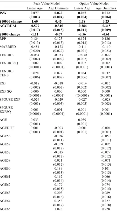
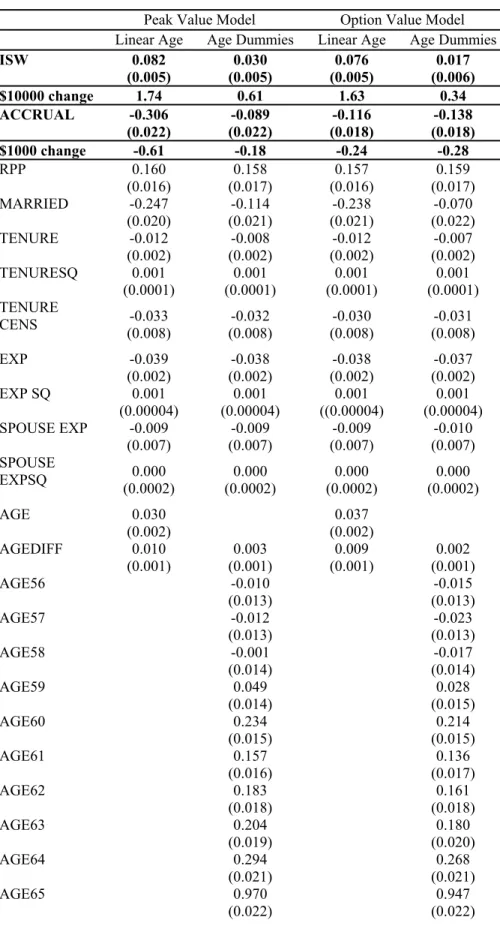
The estimates that form the basis of our policy simulations are presented in tables 1 and 2 for males and females respectively. For each measure of accrual we report results from specifications that alternatively include linear controls for age or age dummies. We also report the impact of a $10,000 change in ISW, or a $1000 change in the accrual measure. For males, the results are uniformly supportive of an important role
for IS incentives in determining retirement. There is consistently a positive and
significant coefficient on ISW, and a negative and significant coefficient on the accrual measure. Conditional on linear age a $10,000 rise in ISW raises the odds of retirement by 1.4 to 2 percentage points, from a base of 14.8%. When, alternatively, age dummies are included, the effect of ISW falls considerably, $10,000 now raising retirement rates by 0.23 to 0.51 percentage points. This drop in the ISW coefficient will be important for understanding the simulation results presented below. The estimates of ACC are also are smaller when age dummies are included, but are less sensitive than ISW. The effects of a change in peak value are roughly half as large, while the estimates for option value are essentially invariant to the inclusion of age dummies.
For females, the estimates for ISW display the same magnitudes and patterns across specifications as the results for men. The estimates of ACC are generally smaller than the results for males but again display the same patterns across specifications.
The estimated coefficients of the age dummies for both males and females display a distinct pattern rising through the early 60’s and peaking at age 65. One possibility is that these dummies are capturing an age-specific pattern of retirement that is due to non-linear changes in the taste for leisure with age, or institutions such as mandatory
retirement that are not otherwise captured in our model. An alternative is that the dummies capture responses to the IS system that are not captured by ISW and ACC. In the latter case we are underestimating the effects of the IS system. As we discuss below, which of the alternatives better capture actual behavior has important implications for the interpretation of our simulation results.
4.0 Simulation methodology
The goal of our analysis is to examine the response of older workers to different counterfactual retirement income systems. To do this, we follow the retirement decisions and retirement income of a cohort of workers from age 55 through the rest of their life under different institutional arrangements. In this section, we first describe the selection of our cohort. Next, we describe the methodology for the calculation of the IS flows, followed by the construction of the labor market exit probabilities. The penultimate subsection discusses our strategy for incorporating spousal response into the analysis. Finally, we describe in detail the structure of the two reforms we consider.
4.1 Cohort Selection
We select the cohort of men and women who were age 55 in 1991 from our full data set. This includes all of the 55 year-old men from 1991, as well as the 55 year-old single females. Married females must be excluded to avoid double counting of
individuals, as our sample of married men will account for their IS behavior. The spouses of our married men are taken without regard to their age. So, the cohort can be defined as a representative sample of Canadian 55 year-old workers in 1991, and their spouses.25 To clarify the discussion that follows, we refer to those in the original sample as ‘cohort members’ and the spouses of the cohort members as ‘spouses’.
Descriptive statistics appear in Table 3. The sample includes 12,058 cohort members, of which 5,050 are married men, 3,662 single men, and 3,346 single women. The average age of the women married to our sample men is 51.5, which is 3.5 years less than the age of the sample men. The men have higher lifetime APE than the women do,
25 Our sample excludes those in primary industries and the self-employed, so it is only representative of the
as well as more job tenure, labor market experience, and a higher probability of employment-based pension coverage.
4.2 Calculating the flows of benefits and taxes
We begin our analysis by calculating the benefit and tax flows that will be
received and paid by cohort members and their spouses from the age of 55 until age 102. Our interest in the IS benefits is obvious – we wish to compare the value of benefits paid out to the cohort under the base and reform IS systems. We account for taxes in order to show the full fiscal impact of the reformed IS systems. If a reform induces workers to stay in the labor force longer, then these workers will pay more in income taxes, payroll taxes, and consumption taxes. These tax effects can have a substantial impact on government balances, as will be shown in our results below.
Taxes pay for public expenditures other than IS benefits, so the level of tax revenue has no meaningful comparison with the level of IS benefits. Instead, the
inferences we will draw come from the difference in tax revenue under different reforms. Presumably, any extra work induced by the reforms would have little impact on other demands for government spending, and so would be a windfall gain to the government’s budget.
The IS and taxation system we consider is the one that prevailed in 1991. The methodology we employ assumes that this system remains constant in real terms into the future. Since 1991, the structure of the IS system remains largely unchanged, although some program parameters have changed since that time.26 This may have some impact on the levels of the IS calculations we make, but our inferences about how IS reform would
change retirement behavior are relevant so long as the structure of the IS system takes the same basic form.
We calculate the three types of taxes in the following way. First, our treatment of income taxes includes both provincial and federal income taxes. Income taxes depend on the level of CPP/QPP benefits, OAS benefits, labor market income, and non-labor
income assigned to each individual in the family under a particular IS system. Payroll taxes are calculated based on labor market income. We account for the CPP/QPP payroll tax and the Employment Insurance payroll tax.27 Both the employer and the employee portions are counted. Finally, for consumption taxes we calculate a consumption tax factor that relates the proportion of consumption taxes to disposable income.28 This factor is applied to the calculated after-tax income of our cohort families to estimate the proportion of their income that will end up as consumption tax revenue.
The assumptions about the impact of changes in work on government revenue are necessarily imperfect. For example, we do not treat the impact that an increase in labor supply might have on corporate profit and the resulting taxation of profit. As well, our treatment of consumption taxes is relatively crude. For these reasons, the resulting calculations should be interpreted only as illustrative of the effect changes in the IS system could have on tax revenues.
26 The 1997 reform of the CPP/QPP system implemented several incremental changes in the calculation of
benefits, but kept the core structure of actuarially adjusted earnings-related benefits replacing about 25 percent of pre-retirement earnings for average workers.
27 In 1991, the CPP/QPP payroll tax was 2.3 percent of earned income between $3,050 and $30,500. This
2.3 percent rate was levied both on employers and on employees, so the total tax rate was 4.6 percent. The Employment Insurance payroll tax was set for 1991 at $2.52 per $100 of earnings up to a cap of $35,360 for employees, and $3.53 on the same base for employers.
28 Personal Disposable Income from the national accounts for 1991 was $473,918 million (CANSIM II
series V691803). Total consumption taxes at all levels of government for fiscal year 1991/1992 was $59,554 million (CANSIM II series V156262). Personal Disposable Income is reported net of indirect
The benefit and tax flows must be calculated for 48 different states of the world, representing the different possible modes of exit from the labor market as described immediately below. The flows will be combined with the probabilities of being in each state to arrive at a value for the PDV of future benefit and tax flows for each family in our selected cohort.
Our point of departure is the observation that each member of the cohort will leave the labor force at some age between 55 and 78. This exit may take place by an exit to retirement or by an exit to death. These differing modes and ages for exit therefore comprise 48 different states of the world. From the point of exit forward, a DNPV calculation of future IS flows can be made to arrive at the ISW associated with each particular labor market exit state. If the probability for each state is known, then the total DNPV of all future IS flows from the point of view of the original cohort when they are 55 can be calculated as an average of the state-specific ISW, using the probabilities as weights in an expected value calculation.
The first task is to calculate the flow of IS payments, income taxes, and CPP/QPP premiums associated with each of the 48 states. We implement this by calculating, for each age between 55 and 102, the IS flows for both the cohort member and the spouse. All future IS flows are discounted back to age 55 for time preference at a real three percent rate. For ages past age 55, we project forward earnings as constant in real terms from age 55.
The flows we calculate are conditional upon the state under consideration. For example, consider the ‘exit to retirement at 67’ state. We assume that the worker is in the
taxes, so the calculated consumption tax factor is [$59,554 million / ($473,918 million - $59,554 million)]=0.1115.
labor force until age 66 and then retires at age 67. We account for benefits and taxes both before and after age 67 -- income taxes, CPP/QPP premiums, and GIS payments may occur in years prior to reaching age 67. We also assume that the worker is alive until at least age 67. In other words, benefits and taxes are received and paid with probability one until age 67, then using the life-tables conditional on having reached age 67 for ages beyond 67. The probability of the worker dying before having reached age 67 will be accounted for in the construction of the probability of being in the ‘exit to retirement at age 67’ state. The output of these calculations is the family level of IS payments, income taxes, and CPP/QPP premiums from the point of view of age 55 corresponding to each of the 48 states.
4.3 Calculating the probabilities
To arrive at the expected value of future IS flows from age 55, we must average the flows received in each state using the probabilities associated with each state. The calculation of the flows associated with each state is described above. The probabilities can be calculated using the output of the models discussed in section 3. For each member of the cohort, we take the member’s observed characteristics (age, province, tenure, etc.) and combine them with the estimated parameters displayed in Tables 1 and 2 to generate a predicted probability of labor market exit. The key component of this calculation is the set of IS incentive variables. We must calculate the IS incentive variables for each potential age of exit, from age 55 to 78. The IS incentive variables can then be combined with the member’s observed characteristics to obtain the predicted probability of labor market exit at each age from 55 to 78.
Predicting retirement after age 69 presents a challenge. Our empirical model estimated the retirement behavior of workers from age 55 to 69. For ages past age 69, we therefore use the conditional probability of exit at age 69 for all ages from 69 on. This assumption has little impact on our overall fiscal measurements, since the probability of remaining in the labor force until age 69 is typically less than one percent in our
simulations. This means that little weight is placed on these labor market exit states. In our data, we cannot distinguish between death and retirement – individuals are observed as long as they receive T-4 forms. To decompose our predicted probability of labor market exit into a probability of exit to retirement and a probability of exit to death, we draw upon the age-contingent life tables. At each age, we subtract the actuarial probability of death at that age from the predicted probability of labor market exit to obtain the predicted probability of retirement for that age.
The next step in computing the state probabilities is to transform the conditional age-specific exit rates to unconditional probabilities for each state. Starting with 100 per cent probability of survival at age 55, the conditional probabilities of exit to retirement and to death at each age are multiplied by the remaining probability of survival. For example, if the probabilities for exits to death and to retirement are 0.02 and 0.05 at age 55, then those probabilities are multiplied by the probability of survival to age 55 (which is 1.0) to arrive at the probabilities for the age 55 states. For age 56, the conditional probabilities for exit at age 56 are multiplied by 0.93, which is the probability that the cohort member survived to age 56 (1.0 – 0.02 – 0.05). This delivers the state
probabilities for age 56. Continuing in this way, the state probabilities for each age to 78 can be calculated.
4.4 Spouses
Spouses add a complication to these calculations. In our previous analysis, we held fixed the spouse’s retirement decision at the first age of eligibility for retirement benefits in order to avoid the complexity of modeling joint retirement decisions. For the simulation calculations we take a similar approach, assuming any spouse retires at the age of first pension eligibility. As a check on this decision, we investigated a more flexible approach on a small subsample. We averaged each of the 48 state probabilities and flows over the 48 possible labor market exit states of the spouse. These simulations showed little change in the retirement incentives of our cohort members compared to simulations with the fixed date of spousal retirement. This reflects two features of our situation. First, there is not a great deal of inter-spousal dependence of benefits in Canada. Second, the assumption of retirement at the date of first eligibility is a good approximation of average spousal behavior. Given this evidence, we proceeded with the use of the fixed spousal retirement assumption.
4.5 Reforms
In addition to performing these calculations for Canada’s existing IS system, we also use this methodology to examine the impact of changes to the IS system. The motivation for analyzing these reforms is not to advocate for a particular structure for Canada’s IS system, but instead to demonstrate the magnitude and shape of the fiscal effects of reforms. We contemplate two possible reforms. The first reform increases all
age-specific entitlement ages by three years. The second involves a shift to a ‘common’ system that is the same across all countries in the project.29
4.5.1 Three-Year Reform
Eligibility for all components of Canada’s IS system is at least partly determined by age. In the Three-Year Reform, we raise the key entitlement ages by three years. For the CPP/QPP, this means that the first possible age of receipt of early retirement benefits is increased to 63, and the normal retirement age is increased to 68. The age of GIS and OAS entitlement also shifts up to 68. Finally, the Allowance is available to qualifying individuals between the ages of 63 and 67.
The Three-Year Reform should affect the level of ISW. Removing three years of eligibility from a worker’s future benefit flows decreases the total value of future flows, meaning a lower level of ISW. Because our models predict a positive wealth effect on retirement decisions, this should lead to a shift toward later retirements.
The effects of this reform on dynamic incentives are both obvious and subtle. The obvious effect is a three-year shift in the age-dependent incentives of the IS system. For example, each dollar of labor market earnings reduce GIS entitlements by 50 cents (single) or 25 cents (married). Under the Three-Year Reform, this large disincentive for continued work is delayed until age 68. Similarly, the dynamic incentives at age 60 due to the availability of early retirement benefits is now delayed to age 63.
More subtly, the Three-Year Reform should also attenuate the magnitude of all dynamic incentives. Any change in the future yearly flow of pension entitlements caused by an extra year of work will have impact over fewer years of pension receipt. This
29 Other countries in this project also simulated a reform with actuarially adjusted benefits. For the case of
suggests that both retirement-inducing and retirement-delaying incentives will be smaller. Combined with the predictions about the effect of the reform on the level of ISW, we expect that the Three-Year Reform will lead to a substantial shift toward later
retirements.
4.5.2 Common Reform
The second reform imposes a common program structure on each country in this project. We therefore refer to it as the ‘Common Reform’. It involves a single, earnings-related public pension. The pension is based on average real lifetime earnings calculated over the best 40 years. We only have 26-year earnings histories for our cohort when we first observe them at age 55,30 so the average is constructed over the number of years of work until they reach 40 years of work, and then the best 40 years thereafter. Wages are converted to constant dollars using a real wage index.31 The amount of the normal pension is set at 60% of the calculated average lifetime earnings. The normal age of retirement in the common reform is age 65. Early retirement benefits are available from age 60, subject to an actuarial adjustment of six percent per year. A survivor benefit is paid, equal to the worker benefit. However, a person is not entitled to both a survivor benefit and a retirement pension at the same time – only the larger of the two is received.
Relative to Canada’s current IS system, the Common Reform eliminates the GIS, Allowance, and OAS benefits. The benefit structure is very similar, however, to that of the CPP/QPP, although with a much larger replacement rate. Because there is no cap to
rendering these simulations uninformative for Canada.
30 Our data includes earnings histories constructed back to the onset of the CPP/QPP programs in 1966.
Our selected cohort is 55 in 1991, meaning that we have only 26 years of earnings for these workers.
31 The real wage index was created using the Industrial Composite Wage from 1966 to 1984, followed by
the Industrial Average Wage from 1984 to 1998, along with the Consumer Price Index. These are derived from Statistics Canada (1983) and Statistics Canada (2000).
pensionable earnings, high earners should receive a much higher pension than they do under the existing Canadian system. In contrast, low earners will do poorly under the Common system, as all benefits become earnings-dependent, in contrast to the existing Canadian system with its earnings-independent demogrants.
The effects of the Common Reform on retirement incentives are not as
straightforward as for the Three-Year Reform. The level of ISW may increase for high earners, but decrease for low earners. With the higher earnings replacement rate, the incentive for extra years of work should be larger than in the existing CPP/QPP where the replacement rate is 25% and capped for high earners. The early and normal retirement ages, as well as the early retirement adjustment of 6% per year coincide exactly with the structure of the CPP/QPP. Finally, the elimination of the income-tested benefits will remove their dynamic retirement incentives.
4.6 The Effects of Age
In section 3, we noted the difficulties interpreting the estimates of the age dummy variables in our empirical models. The ambiguity is potentially very important for our simulations of the Three-Year Reform in which we change the age structure of the IS incentives. As a consequence we implement two strategies that imply very different interpretations in investigating this reform. In the first, we do not shift the age dummies as the entitlement ages increase. Here we assume that any age specific propensities for retirement as captured by the age dummies are independent of the parameters of the IS system. In the second strategy, we instead shift the age dummies three years forward in parallel with the shift in program eligibility ages. The estimated coefficient on the age 55 dummy becomes the dummy for age 58, the age 56 dummy becomes the dummy for age
59, and so on.32 Here we allow the possibility that the age dummies capture latent effects of the IS system, and so are sensitive to the age parameters of the IS system.
4.7 Decomposition
The total effect of reforms to Canada’s retirement income system can be
decomposed into two effects. To show this, we first express the total effect of the reform as the difference of the ‘reform’ IS flows and the ‘base’ IS flows:
. 48 1 48 1
∑
∑
= = − = s B s B s s R s R s ISW P ISW P effect TotalThe superscripts R and B index the reform case and the base case. The labor market exit states are indexed by s. For each state s, there is a probability Ps and a discounted flow of
IS payments, ISWs.
We decompose the total effect by adding and subtracting a term that combines the reform IS payments and the base probabilities:
. 48 1 48 1 48 1 48 1 − + − =
∑
∑
∑
∑
= = = = s B s B s s R s B s s R s B s s R s Rs ISW P ISW P ISW P ISW
P effect
Total
The second bracketed term we call the mechanical effect. It measures the difference in the discounted flows between the new and the old IS systems, holding retirement behavior constant. This is the cost to the treasury of increased (or decreased) pension payments with an assumption of static behavior. The first bracketed term we call the
fiscal implications of the behavioral effect. Here, holding ISW constant, we measure the effect of the change in the timing of retirement induced by the reform.
5.0 Results
We present three simulations for each of two measures of retirement incentives. The first simulation is based on the estimates for the empirical model with the linear control for age. The second is based on the estimates for the model with age dummies, but assumes that the effect of age as captured by the estimates of the dummies does not shift in tandem with the reforms (as discussed in Section 4.6). Finally, in the third we again use the age dummy model, but assume the effects of age shift upwards by 3 years in the Three-Year Reform. Finally, for each of these simulations we present both peak value and option value results.
The main results appear in Tables 4 and 5. Going down each table, the six panels correspond to the six simulations outlined above. Going across Table 4, we present the simulated levels of benefits and taxes under the base system as well as the reform systems. Going across table 5, the total change is decomposed into its behavioral and mechanical components. Within each panel, we show the total PDV of benefits and taxes separately. In table 4, the tax total is broken down into its payroll, income, and
consumption components. All values have been converted to 2001 Euros, using the December 31, 2001 exchange rate of C$1.4185 = €1.00.
5.1 Base system results
In the first column of Table 4 we present the base IS system results. For the peak value – linear age simulation, the PDV of benefits totals €111,106 per working family. The payroll tax total of €15,202 is lower than may be the case for other countries, reflecting Canada’s relatively small rates of payroll tax. To put this in context, a single worker earning the average industrial wage in 1991 would have generated payroll tax
revenue for the government in the 1991 fiscal year of about €2,704. The PDV of income taxes for the average family in our cohort is €81,687. Taking the difference of taxable income and the taxes paid by the cohort families, we estimate a total PDV of after-tax income of €337,225. When multiplied by the consumption tax factor of 0.1115, we arrive at the estimate for the DPV of consumption tax revenues of €37,595. The total DPV of the three sources of tax revenue generated by the cohort families from age 55 on is €134,485.
While the total tax revenue is larger than the future benefits, it must be recalled that tax revenue funds other government spending in addition to the IS system. As well, the tax revenue generated by the family before age 55 is not included in this calculation. For these reasons, no inferences about the sustainability of Canada’s IS system can be drawn from these totals.
Looking down the six panels in Table 4, there is little variation in the calculations across simulations. The age dummy simulations with and without the shift are identical for the base case because the age dummies do not shift in calculating the base case exit probabilities.
5.2 Three-Year Reform
The Three-Year Reform raises all of the critical entitlement ages in the IS system by three years. Figures 1 and 2 show the age profile of the PDV of benefits and taxes, respectively. Two observations are noteworthy. First, the age profile of IS benefits is quite flat. This reflects the actuarial adjustment made to CPP/QPP benefits, and the fact that OAS and GIS benefits are paid independent of participation in the labor market. In contrast, the age profile of taxes slopes upward steeply. Lifetime taxes are higher for
those exiting the labor market at older ages because they have more years of labor market earnings that are subject to income and payroll taxes. The second observation relates to the differences between the base case and Three-Year Reform. The gap between the base case and the reform case diminishes with age. This is generated by the fewer years of expected future pension receipt for those retiring later.
The peak value – linear age panel of Table 4 reveals that this reform would cut benefit levels to €91,328, which is 17.8 percent less than the base IS system level of benefits. However, all three types of tax revenue for the government would increase under the reform, with the total rising by 6.8 percent. This increase is driven by a large increase in payroll tax and income tax revenues.
Underlying these increases in tax revenues is an increase in work generated by the reform. This can be seen clearly in Figure 3. The distribution of retirement ages shifts out to the right, as the reform provides incentives to spend more years in the labor force. The incentive is provided both by the wealth effect of lower lifetime IS benefits, and by an increase in the average peak value dynamic incentive measure as the age at which peak benefits are reached moves to older ages.
In Table 5, the total changes are broken down into the mechanical effect and the behavioral effect. Benefits drop mostly because of the mechanical effect. With no change in behavior, the government will save money by paying three fewer years of pension benefits. The small behavioral effect reflects the approximate actuarial fairness of the CPP/QPP system. Even though workers are retiring later, the DPV of their benefits changes little.
The extra work generated by the reform has a larger impact on tax revenues. Overall, tax revenues increase by €9,083. The mechanical effect is negative, as taxable income falls with the decrease in lifetime IS benefits. However, the behavioral effect captures the increase in government revenues generated by the increased work under the reform.
The importance of considering tax revenues is made clear in Figure 4. We graph the total effect by age, for both the gross ISW benefits and the net of taxes ISW. The gross ISW in the darker bars is negative through age 63, reflecting the mechanical savings and the behavioral savings as retirement shifts later. However, starting at age 64, the total effect on gross IS benefits becomes positive. This is generated by the behavioral effect. Under the reform, there is now more retirement at later ages than under the base case. This increases the cost of IS benefits to the government for those retiring at later ages.
The light bars in Figure 4 show the PDV of IS benefits less the PDV of taxes. Even when the gross IS benefits show a cost to the government after age 63, the light bars still show an overall decrease in the government’s fiscal outflow. The difference is the extra work that is generated by the reform. Those who are shifting to retirement at later ages now work more years, which generates more tax revenue for the government. So, even though the actuarially adjusted IS benefits of later retirees costs the government more, the taxes they pay until they retire overcompensates for the increased IS benefit cost.
Overall, the net fiscal balance of the government under the Three-Year Reform changes by €28,860 per family, or 26 percent of the base level of benefits. Importantly,
almost half of the 26 percent change is accounted for by the behavioral effect. In other words, an analysis that assumes static retirement behavior would underestimate the fiscal effects of the Three-Year Reform by about half.
The age-dummy simulations are quite informative for the Three-Year Reform. Looking first at Table 4, the predicted benefit level for peak value in the age dummy simulations is approximately the same as for the linear age simulation. The taxes, however, show some differences. For the no-shift simulation, the total taxes increase by only 0.7 percent, compared to 6.8 percent for the linear age simulation. The with-shift simulation shows an increase of 4.3 percent in tax revenues.
An explanation for these tax revenue differences can be found in Table 5. The mechanical effect for the two dummy-shift simulations is identical, as expected. In the no-shift simulation, the behavioral effect is driven only by the changes in IS incentives. Here, the behavioral effect on taxes is smaller than in the linear-age case at €5,716. However, for the with-shift simulation the behavioral effect is nearly twice as large, at €10,451. This suggests that the shift in the age dummies generates only half of the behavioral effect. In other words, even with the seemingly strong assumption that age-related retirement propensities do not change when the normal retirement age changes, we still generate a substantial behavioral effect for taxes of €5,716 per family.
The overall net fiscal savings for government implied by the two age-dummy simulations is 18.6 percent of base benefits for the no-shift case and 22.8 percent for the with-shift case. The two biggest contributors to these changes are the mechanical effect on benefits as workers are entitled to fewer years of benefit receipt, and the behavioral effect on taxes as workers have higher lifetime earnings.
The option value simulations in the bottom three panels of Tables 4 and 5 show a similar pattern as the peak value simulations for the Three-Year Reform. The overall change in net benefits as a percent of base benefits is 22.3 percent for the linear-age simulation. For the age-dummy simulations, the no-shift case shows a smaller behavioral effect than the with-shift case.
We present the mechanical and behavioral effects for all six simulations as a percentage of 2001 GDP graphically in Figure 7. Our sample is based on a 10 percent sample of the Canadian labor force outside the primary sector, so we arrived at the totals by summing over all 12,058 cohort members and multiplying by ten. The behavioral effect totals €1.7 billion and the mechanical effect totals €1.8 billion for the peak value – linear age simulation. Together, the two effects sum to about 0.45% of Canada’s €770 billion GDP in 2001.
For both peak value and option value, the largest behavioral effect is found in the linear age specification. In both cases, this is caused by a larger wealth effect driven by a higher estimated ISW coefficient. The second and third bars show the difference
between the age dummies results with and without the age dummy shift. As these two cases represent the two extreme assumptions for the treatment of the age dummies, they therefore bound the magnitude of the behavioral effect in the age dummies simulations.
5.3 Common Reform
The Common Reform gives workers a benefit based on 60 percent of the average of their best 40 years of lifetime earnings. Table 4 reveals that this reform has a large wealth effect. For the peak value linear-age simulation, the level of benefits increases by 73.3 percent. The extra taxable income generated by the higher benefits leads to
increases in income tax revenue and consumption tax revenue. However, payroll tax revenue declines under the reform. This suggests that the reform decreases the amount of work; that it leads to earlier retirement.
Figures 8 and 9 explore the Common Reform graphically. First, Figure 8 shows the dramatic increase in IS benefits under the reform. Figure 9 shows the shift to earlier ages of retirement in the distribution of retirement ages under the option value - linear age specification. We look into the source of this large shift to earlier retirement ages below.
In Table 5 we decompose the total effect of the Common Reform into the
behavioral and mechanical effect. For benefits, the mechanical effect is much larger than the behavioral effect. The benefits paid under the Common Reform, at 60 percent of lifetime earnings, replace a higher proportion of earnings than the existing Canadian IS system. Like the Three-Year Reform, the larger behavioral effects can be seen in tax revenue. For the peak value – linear age simulation, tax revenue falls by €7,944 per family because of the behavioral effect. With the age dummy simulation, however, the drop in tax revenue is reversed.
The explanation for this difference lies in relative strengths of the wealth effect and the dynamic incentive effect. The average value for peak value over our sample in the base case was €779. With the Common Reform, this increased to €4,370. Given the negative coefficient on peak value in Tables 1 and 2, this implies a shift toward later retirement. In contrast, the wealth effect of the Common Reform shifts retirement in the other direction, as more wealth leads to a desire to retire earlier. However, as can be seen in Tables 1 and 2, the magnitude of the coefficient on ISW falls dramatically between the
linear age and the age dummy estimates, from 0.077 to 0.022 for males and similarly for females. So, the wealth effect of the Common Reform dominates the dynamic effect for the linear age simulation, but with the small estimated coefficient on ISW for the age dummy simulation, the dynamic incentive effect is able to dominate the wealth effect and retirement pushes later.
For the option value simulations, the decrease in work under the reform is stronger. Again, the wealth effect of ISW leads to earlier retirement. However, in contrast to the peak value case, the dynamic incentive of the option value is not able to overcome the wealth effect. So, the net effect is a larger decrease in work. The
difference between the linear age and age dummy simulations for option value are driven by the same factor as for peak value – the change in the ISW coefficient in Tables 1 and 2.
6.0 Distribution
In addition to looking at the shifts in behavior and the fiscal costs of IS reform, we can use our simulation models to examine how the two reforms affect distribution of IS payments. We split our cohort families into quintiles based on the average lifetime income index described above for the Common Reform. For married families, we use the sum of husband and wife income. For single cohort members, we use only the member’s income. We rank the families based on this income measure separately for married and single families, so that an equal proportion of married and single families is in each quintile. The highest income quintile of the single group is combined with the top one fifth of families from the married group to comprise Quintile 1. Quintiles 2 through 5 are formed in a similar way, progressing to the lowest income households in Quintile 5.
Table 6 presents the distributional analysis for the option value – linear age simulations, and Table 7 the option value – age dummy (with shift) simulations. The five quintiles appear in the five panels of each table. Across the table, we present the levels of the PDV of benefits and taxes, as well as the changes relative to the base for each reform.
The linear age simulations in Table 6 show that the base PDV of benefits is remarkably stable across quintiles. This stability reflects several aspects of Canada’s IS system. First, only earnings up to the YMPE are insured by the CPP/QPP pensions. Since the YMPE is set close to median earnings, this means that lifetime earnings above the median will result in no additional CPP/QPP benefits. Second, the only part of the Canadian system that is related to lifetime earnings is the CPP/QPP component – and it replaces a smaller share of the total IS system than do earnings-related benefits in other countries. Third, the income-tested components of the IS system tend to compensate those with lower lifetime earnings. Finally, higher income individuals will be subject to higher rates of income taxation as well as potentially facing the clawback of OAS
benefits. Combined, these factors make the profile of IS benefits very flat with respect to changes in lifetime earnings.
Taxes, on the other hand, show a progressive pattern. The larger tax levels in the higher income quintiles reflect higher levels of CPP/QPP benefits, labor income while still in the labor force, and non-labor income. As we move down the table to the lower income quintiles, these sources of income are replaced with non-taxable GIS and SPA benefits.
The Three-Year Reform does not dramatically alter this pattern of distribution. Benefits are relatively flat across the earnings distribution, while taxes increase sharply
with lifetime earnings. The net benefits drop in all quintiles. The percentage decrease follows a monotonic pattern with the highest decrease in the first quintile and the lowest decrease in the fifth quintile. This suggests that a reform to delay benefit receipt by three years may be progressive.
The Common Reform has a very different impact on distribution. First quintile households have their insurable earnings capped at a much higher level under the Common Reform than is the case in the status quo CPP/QPP, resulting in much higher benefits. The first quintile households have almost no changes in their taxes, however. This result stems from the huge wealth effect on retirement implied by the large
estimated ISW coefficient combined with the large change in ISW. Government tax revenue does not increase because they lose income and payroll taxes on the labor that is no longer provided by this quintile. Overall, the effect on the first quintile is a net increase of 156.2 percent over base benefits.
Farther down the income distribution, the effect of the Common Reform is far less generous. For the fifth quintile, the replacement of the income-tested benefits and the OAS demogrant by a pure earnings-related benefit decreases the average level of benefits by one third. This has a wealth effect on their labor supply, causing them to work more. This generates more income and payroll tax revenue for the government than in the base case for this quintile. These households suffer a drop of 37.8 percent of base benefits under this reform.
The distribution analysis is repeated for the option value – age dummy simulations in Table 7. The patterns are very similar to those in Table 6 using peak value. The primary difference lies in the smaller magnitudes of the responses to the