Fiscal rules and structural reforms

ADEMU WORKING PAPER SERIES

Fiscal Rules and Structural Reforms

Rana Sajedi

Armin Steinbach

May 2018

WP 2018/133

www.ademu-project.eu/publications/working-papers

Abstract

Implementation of _scal surveillance rules relies heavily on the proper interpretation of legal terms,

creating a need to infuse economic insight into legal analysis. Rigid legal application of fiscal

deficit rules may curtail structural reforms, as reforms can go against fiscal consolidation in the

short run. However, if reforms are expected to improve public finances in the long run, they should

not be viewed as incompatible with the legal framework. Focussing on the case of EU fiscal

surveillance, this paper identifies the circumstances under which the positive budgetary long-term

effect of structural reforms materialize in such a way that the legal rules should be applied with a

degree of leniency, allowing for a short-term deterioration of the fiscal position. To that end, we

quantify the short-run fiscal costs and long-run fiscal benefits of reforms, and investigate how the

design of reforms can affect this trade-off. Results suggest that as short run output losses of

reforms are alleviated by fiscal stimulus, long run output gains from the reforms imply that fiscal

viability can be reached within a reasonable period of time. Product market reforms are generally

preferable over labour market reforms, as they have a larger impact on fiscal revenues. These

insights inform the legal analysis in several regards. First, the economic analysis is in line with

teleological interpretation of legal rules aimed at ensuring long-term fiscal stability, while allowing

short-term fiscal leniency. Second, the economic analysis can give contours to vague legal terms,

such as ‘prompt’ positive budgetary effects and the legal requirement of ‘major’ structural reforms,

showing that the type of reform matters as much as the size of the reform, and that while larger

reforms have larger long run budgetary effects, they also require greater leniency in the short run.

More generally, our analysis calls for the design and interpretation of legal fiscal regimes with

reference to the interdependency between fiscal policy and structural economic policies.

† _{Bank of England, [email protected]}

Acknowledgments

This project is related to the research agenda of the ADEMU project, “A Dynamic Economic and

Monetary Union". ADEMU is funded by the European Union's Horizon 2020 Program under grant

agreement N° 649396 (ADEMU).

_________________________

The ADEMU Working Paper Series is being supported by the European Commission Horizon 2020 European Union funding for Research & Innovation, grant agreement No 649396.

This is an Open Access article distributed under the terms of the Creative Commons Attribution License Creative Commons Attribution 4.0 International, which permits unrestricted use, distribution and reproduction in any medium provided that the original work is properly attributed.

1

Introduction

Application of fiscal rules is often considered in clinical disciplinary isolation. While lawyers tend to care about dogmatic consistency and uniform application of rules, economists are concerned about the effects of the specific design of fiscal rules. However, legal interpretation and economic effects interact and a legal analysis being informed about the economic effects associated with certain ways of legal interpretation may tune the overall application of rule enforcement. The recent EU debt crisis has brought to the forefront the need for lawyers and economists to relate their disciplinary contributions to each other. Disrespect of fiscal rules has been widely recognized as a major cause for sovereign debt turmoils in the recent Euro-area crisis and the austerity measures imposed as response to the crisis follow the logic of fiscal retrenchment. At the same time, an insufficient level of structural reforms remains a perennial phenomon in the EU. Some of these reforms are critical for the growth and sustainability of the Euro-zone as a whole, as they imply positive externalities across countries (European Commission 2014). By design, fiscal regimes are established with the aim to constrain public expenditures and policy maneuver, for which there may be sound economic reason: the negative spillover effects from sovereign debt on other members of a currency union (Antonakakis and Vergos 2013); political economy insight that political decision-makers’ focus on re-election undermining fiscal discipline to the detriment of future generations (Beetsma and Debrun 2004, Poplawski Ribeiro and Beetsma 2008); and negative impact on growth inflicted by fiscal burden (Panizza and Presbitero 2014). However, strict application of fiscal rules may be counter-productive in cases where economic policy measures may improve the fiscal stance in the long-term, the short-term fiscal burden notwithstanding. This applies particularly to two instances: First, public investment may stimulate growth and thus improve the debt-to-GDP situation, while giving rise to numerous controversial issues regarding nature, size and crowding-out (Mourougane et al. 2016). Second, structural reforms are widely claimed to be necessary in order to foster growth (Griffith and Harrison 2004, Griffith et al. 2007, Fiori et al. 2012, International Monetary Fund 2017), while less attention has been given to the fiscal implications of structural reforms.

This study relates to the latter strand of literature by examining the interaction between legal and economic insight in the relationship between fiscal rules and structural reforms. The analytical approach is to indicate avenues of legal interpretation by incorporating economic analysis on the impact of structural reforms on a country’s fiscal position. This analysis seeks an economic interpretation of the EU rules governing fiscal conduct and highlights how legal interpretation can be informed by economic insight. Legal and economic questions in the domain of fiscal governance interact.

Relevant legal questions are: How can fiscal rules be interpreted to the extent that structural reforms should be accounted for under the fiscal governance regime? Can fiscal leeway be granted in exchange for structural reforms? And how can certain vague legal terms – such as “prompt” positive budgetary effect of structural reforms or “major” structural reforms – be interpreted with a sound economic rationale? These legal questions can be addressed through economic analysis. To understand whether a government should invest time and public expenditure on the costs of structural reforms, it is important to compare the potential short run fiscal costs to the effects of those reforms on public finances in the long run. In particular, reforms which boost economic growth can improve the fiscal balance in the long run, and so be self-financing despite the fiscal costs in the short run. Methodologically, this can be

Based on our theoretical framework, we show that economic analysis supports the leeway to account for the im-plementation of structural reforms identified through legal reasoning. We identify the circumstances under which the positive budgetary long-term effect of structural reforms are such that the legal rules should be applied with a degree of leniency allowing for a short-term deterioration of the fiscal position in return for greater long-term fiscal position. We further provide economic meaning to the legal terms “prompt” (related to the timely positive budgetary effect) and “major” (related to the size of the reform).

Hence, the article aims at offering a three-fold contribution: First, it modifies the seemingly opposing position of fiscal stance and (costly) structural reforms by adding analytical differentiation with regard to size, type and dynamic effects of structural reforms. Second, the analysis reveals the economic underpinning of legal rules on fiscal governance and offers insight which can inform political decision-making on the enforcement of fiscal legal rules. Third and on a general note, it highlights how economic insight can be used for a genuine legal interpretation exercise, which underscores the argumentative force of holding legal terms susceptible for interdisciplinary transfer. The article is structured as follows: the next section lays out the framework for the legal analysis and the open legal questions around the interplay between fiscal rules and structural reforms. The third section details the economic analysis used to inform those questions, and the fourth section takes those economic insights back to the legal analysis.

2

Legal Analysis

At its core, the issue is that strict compliance with fiscal numerical rules, at least in the short run, seem incompatible with the fiscally contractionary effect of structural reforms. Thus, allowing flexibility and leniency in the fiscal regime in favor of structural reforms rests on the assumption that structural reforms improve (or at least do not alter) the fiscal stance of a country. This raises a number of questions: To what extent do structural reforms alter the fiscal position of a country? What is the short-term versus long-term effect of structural reforms on the fiscal position? Do size and type of the structural reforms matter?

These economic questions are embedded into a legal framework. The EU offers a suitable case to study the interaction of legal and economic questions. More specifically, the Stability and Growth Pact (SGP) is the key instrument of fiscal policy coordination, featuring binding rules and sanction mechanisms (Steinbach 2013, 28; De Grauwe 2016, 218-224). In the past, application of the SGP focused on fiscal policy and compliance with numerical budget rules. Even though the rules have not always been applied consistently due to political reasons (Fat´as and Mihov 2010), there is a strong conviction in legal scholarship (Borger 2016, Palmstorfer 2012) and economic scholarship towards strict enforcement of fiscal rules. This stance has been subject to criticism pointing, inter alia, at other elements promoting growth and positive long-term budgetary effects, such as structural reforms. The call for structural reforms was broadly raised by IMF, OECD and the EU Commission (European Commission 2015a).

In principle, under EU rules the fiscal regime allows integration of non-fiscal considerations on two stages of the fiscal surveillance. Under the preventive arm of the SGP (i.e. ensuring sound budgetary policies over the medium term), the relevant legal provision explicitly states that the Commission and Council shall “take into account the implementation of major structural reforms” when defining the adjustment path to the medium-term budgetary

objective.1 _{Thus, “major structural reforms” may, under specific circumstances, justify a temporary deviation from}

the medium-term budgetary objective of the concerned Member State or from the adjustment path towards it. Less clarity, however, exists as regards the relevant norms of the corrective arm (i.e. correction of excessive deficits). The relevant norms are silent on the treatment of structural reforms. The only legal term potentially allowing the incorporation of structural reforms into the assessment under the corrective arm states that the Commission “[. . . ] shall take into account all relevant factors [. . . ] in so far as they significantly affect the assessment of compliance with the deficit and debt criteria by the Member State concerned”.2 The reference to “relevant factors” has been interpreted by the Commission as including the implementation of structural reforms (European Commission 2015b, p.13).

The legal terms have been subject to legal interpretation and implementation. To that end, the Commission has set out a number of principles to be followed for the structural reforms clause to be activated (European Commission 2015b, p.11). First, the Commission has stressed the wide margin it enjoys when assessing the soundness of public finances in the light of country-specific circumstances. Indeed, the European Court of Justice has confirmed that the Commission enjoys wide discretion in the assessment of economic circumstances.3 This reflects the general perception in legal scholarship that the executive branch enjoys a certain margin of discretion. Also, another legalistic approach to interpretation is to account for the “purpose and spirit” of legal rules as element of a teleological method of interpretation (Lenaerts and Guti´errez-Fons 2014). There is no indication that interpreting structural reforms as “relevant factors” would be incompatible with the overall purpose of the excessive deficit procedure, which is to ensure the correction of excessive deficits, i.e., making sure that Member States return to a sustainable fiscal position.

Second, on the basis of its discretion, the Commission found that structural reforms can be recognized provided they have a long-term positive budgetary effect where this effect can have direct budgetary savings from reforms (e.g., pension reform) or through increased revenues (e.g., as a result of increased employment). This interpretation of the fiscal rules can be explored by economic methods and forms part of the analysis below.

Third, the legal text requires reforms to be “major” in relation to their effect on growth and the sustainability of public finances. Requiring a significant impact enables the EU Commission to request sizeable and effective reforms and the appropriate choice of policy mix. Again, the soundness of this requirement can be assessed through economic modelling.

Finally, according to the legal requirement, structural reforms must account for the main purpose of the corrective arm of the SGP, which is to ensure the “prompt” correction of excessive deficits.4 _{This criterion corresponds to the}

dynamic adjustment occurring between the implementation of structural reforms and the new post-reform fiscal steady state and can also be determined through economic modelling.

1_{Article 5 of Regulation (EC) no. 1466/97} 2_{Article 2 of Regulation (EC) 1467/97}

3_{See only, Case T-201/04 Microsoft v Commission [2007] ECR II-3601, para. 87; Case T-168/01 GlaxoSmithKline v. Commission} [2006] ECR II2969, para. 57.

4_{Further, the wording of the relevant legal provision requires the “implementation” of structural reforms, referring to effectively} implementing conditionality in order to incentivize actual implementation (not just the announcement) of structural reforms.

3

Economic Analysis

The above legal requirements and interpretations can be subject to an economic review by re-phrasing the legal reasoning in economic questions: Do structural reforms alter the deficit-to-GDP both in the short and long run? Only if so, there is rationale to discuss the integration of structural reforms into the fiscal regime, because if, in the short-run, deficit-to-GDP increases, this would require flexibility in the enforcement of fiscal rules. And if, in the long run, structural reforms lead to lower post-reform deficit-to-GDP ratio compared to non-reform scenario, this offers rationale for granting leeway due to a better ex-post fiscal position. We will further refine the analysis by exploring the effect of fiscal stimulus counteracting the contractionary output effect of structural reforms. Moreover, we will examine the criterion of “major” structural reforms and “prompt” correction of excessive deficits. In particular, we will assess how the size of the reform corresponds to the fiscal stance and we will extend the analysis to whether the type of structural reforms (labour or product market reforms) matters. Finally, the “prompt” requirement can be explored with a view to how much time the fiscal adjustment process takes following the implementation of structural reforms and whether the delay in fiscal recovery can be understood as fulfilling the “prompt” requirement.

3.1

Model

The model closely follows that of Sajedi (2018) and Eggertsson et al. (2014), henceforth EFR. The economy consists of a two-block monetary union, with each block producing tradable and non-tradable goods. In each sector, there exist competitive firms using sector-specific labour to produce intermediate goods. That labour is aggregated from the differentiated labour supplied by households, and imperfect substitution between those labour types leads to a mark-up on wages. Monopolistically competitive firms use the intermediate goods to produce differentiated goods, which they sell with a price mark-up. Households receive utility from an aggregate consumption good, which consists of non-tradables and both domestically-produced and foreign-produced tradables, as well as disutility from labour. As well as issuing debt, the government collects taxes to finance transfers and wasteful consumption expenditures. The following is an exposition of the ‘Home’ block of the union, which has relative sizeσ. The ‘Foreign’ block, of size (1−σ) follows the same structure.

3.1.1 Household

There is a representative household, made up of a continuum of agents of mass σ, which derives utility from aggregate consumption,ct, and disutility from aggregate labour,nt, with expected lifetime utility given by:

E0 ∞ X t=0 βtU(ct, nt) =E0 ∞ X t=0 βt " c1t−η 1−η − n1+t ϕ 1 +ϕ # (1)

whereβ is the discount factor,η is the inverse of the intertemporal elasticity of substitution andϕis the inverse of the Frisch elasticity of labour supply. The final consumption good is an aggregate of the tradable and non-tradable goods, given by:

ct= (1−θ)1ξ_c ξ−1 ξ T t +θ 1 ξ_c ξ−1 ξ N t ξ−1ξ

where the tradable consumption good is itself aggregated from domestic and foreign produced goods: cT t= (1−α)1φ_c φ−1 φ Ht +α 1 φ_c φ−1 φ F t φφ−1

whereαcaptures the openness of the country (the inverse of the home-bias), andφis the elasticity of substitution between domestic and foreign goods. The intertemporal budget constraint is given by:

(1 +τc)ct+bGt+1+bF t+1≤(1−τn)wtnt+ RHt−1 πt bGt+ RF t−1 πt bF t+ (1−τp)mt+Tt (2)

where bGt and bF t are the real holdings of domestic government bonds and foreign bonds, RHt and RF t are the gross nominal interest rates on those bonds, πt is the gross inflation rate of the CPI, defined below, wt is the real wage, averaged across sectors, mt are the profits from the monopolistically competitive firms, which will be discussed below, τc_{, τ}n _{and τ}p _{represent taxes on consumption, labour income and firm profits respectively, and} Tt is a lump-sum transfer from the government. The household delegates the labour supply decision to a labour union, which will be discussed below, and so takesntas given. Thus the household choosesct, bGt+1 andbF t+1 so

as to maximise lifetime utility (1), subject to the budget constraint (2) in every period.

For the optimal level of the final consumption goodct, the households choose the components, cN t, cHt and cF t to minimise their expenditure, given the respective prices PN t, PT t and PT t∗ . Firstly, for a given cT t, the cost minimisation yields the following demand functions for home- and foreign-produced tradable goods:

cHt= (1−α) PT t PT t −φ cT t and cF t=α P_{T t}∗ PT t −φ cT t

wherePT t is the aggregate price of the tradable consumption bundle, defined as:

PT t= [(1−α)P 1−φ T t +α(P ∗ T t) 1−φ ]1−1φ

Then, similarly, the composition of tradable and non-tradable consumption satisfies the following demand functions:

cN t= (1−θ) _P N t Pt −ξ ct and cT t=θ _P T t Pt −ξ ct

wherePtis the aggregate price of the final consumption bundle, the CPI, defined as: Pt= [(1−θ)PN t1−ξ+θP 1−ξ T t ] 1 1−ξ 3.1.2 Production

For simplicity, the exposition of the steps of production will focus on sectork=T, N, withθT ≡θandθN ≡(1−θ) denoting the size of each sector.

Retailers A competitive retailer aggregates a continuum of differentiated goods, indexed byi∈[0,1], as follows: ykt= " 1 θk _k1 Z θk 0 ykt(i) k−1 k _di #_kk−1

wherek is the elasticity of substitution between the different varieties. LettingPkt denote the price at which the retailer sells the final good ykt, and Pkt(i) denote the price at which they buy each good ykt(i), the profit of the retailer can be written as:5

Pktykt−

Z θk

0

Pkt(i)ykt(i)di The zero-profit condition therefore defines the aggregate price as:

Pkt= 1 θk Z θk 0 Pkt(i)1−kdi !1−1k

The cost minimisation of this transaction yields the following demand schedule for each differentiated good:

ykt(i) = 1 θk Pkt(i) Pkt −k ykt (3)

Monopolistic Firms There is a measure of massθk of monopolistic firms that buy intermediate goods at unit priceM Ckt, and differentiate them with a technology that transforms one unit of intermediate goods into one unit of differentiated goods. Following Calvo (1983), in any given period each firm can reset their price with a fixed probability (1−χp). A firm, i, that is able to reset their price chooses the optimal price level, ˜Pkt(i), so as to maximize expected profits given by:

Et ∞ X s=0 χs_pΛt,t+s ˜ Pkt(i)−M Ckt+s ykt+s(i)

subject to the demand schedule, (3), where Λt,t+s is a stochastic discount factor and ykt(i) is the output of firm i. Since all firms are ex-ante identical, all optimising firms will choose the same price, that is ˜Pkt(i) = ˜Pkt. The resulting expression for ˜Pkt, is:

˜ Pkt= k k−1 EtP ∞ s=0χ s pΛt,t+sM Ckt+sykt+s(Pkt+s) k EtP ∞ s=0χspΛt,t+sykt+s(Pkt+s) k−1 (4)

Intermediate Goods Firms Intermediate goods,xkt, are produced with a linear technology using sector-specific labour, xkt = nkt. For a given aggregate nominal wage, Wkt, the firm’s profit maximisation yields the standard first order condition:

Wkt=M Ckt

The labour input is aggregated from the differentiated labour supply of different members of the household, according to: nkt= " 1 θkσ _γk1 Z θkσ 0 nt(j) γk−1 γk _dj #_γkγk−1

whereγk denotes the elasticity of substitution between different labour types, andθkσis the mass of agents working in sectorkin the Home economy. The aggregate wage index is given by:

Wkt= 1 θkσ Z θkσ 0 Wt(j)1−γkdj !1−1γk

The cost-minimisation problem of the firm gives the following demand schedule for each type of labour:

nt(j) = 1 θkσ Wt(j) Wkt −γk nkt forj∈k 3.1.3 Labour Union

The households delegate the labour supply decision to a labour union. As with price-setting, in any given period the union can reset the wage of each household with a fixed probability (1−χw). When they are able to reset wages, the labour union chooses the optimal wage so as to maximise agent’s utility, subject to the intermediate firm’s demand for each labour type, in the relevant sectork.6 _{Hence, the problem of the labour union is:}

max ˜ Wt(j) Et ∞ X s=0 (βχw)s ct+s(j)1−η 1−η − nt+s(j)1+ϕ 1 +ϕ subject to: (1 +τc)ct+s(j) = (1−τn) ˜ Wt(j) Pt+s nt+s(j) +X nt+s(j) = 1 θkσ ˜ Wt(j) Wkt+s !−γk nkt+s

where the first constraint is the agent’s budget constraint, with irrelevant terms subsumed inX. As with prices, with ex-post symmetry, this gives the following forward-looking expression for optimal wages:

˜ W(1+γkϕ) kt = γk γk−1 EtP∞s=0(βχw)sW γk(1+ϕ) kt+s _n kt+s θkσ 1+ϕ EtP ∞ s=0(βχw)sλt+s(1−τn)wkt+sW (γk−1) kt+s (nkt+s/θkσ)

6_{Since the union maximises the household’s utility, this is equivalent to the formulation in EFR, and is still optimal from the} perspective of the household.

3.1.4 Government

The government’s expenditures consist of purchases of domestic non-tradable goods, gt, and lump-sum transfers, Tt, while revenues come from labour income taxes, consumption taxes, and profit taxes. The government deficit is therefore given by:

dt= PN t

Pt

gt+σTt−τn(wT tnT t+wN tnN t)−τcct−τp(mT t+mN t) The budget constraint is defined by:

RHt−1

πt

bGt+dt=bGt+1

When active fiscal policy is considered, government consumption expenditures react to the output gap, defined as the deviation of output from its steady state. Specifically, expenditures-to-GDP evolve according to:7

gt yt = _g y yt y −ρy

This counter-cyclical rule means that fiscal policy is acting to stabilise the economy just as the interest rate might with a Taylor rule. Notice that in the exercises below, unlike in the standard use of stabilisation rules, it is a change in the steady state value of output that gives rise to a non-zero output gap. To ensure stationarity of government debt, transfers respond to deviations of debt from its steady state value, according to the rule:8

Tt=T _b Gt bG ρB 3.1.5 Equilibrium

Aggregating the output of the monopolistic firms, plugging in the demand schedule, yields: xkt=ykt∆kt

where the index of price dispersion is defined as:

∆kt≡ Z θk 0 Pkt(i) Pkt −k di

Under the Calvo-pricing assumption, the price index can be written as:

Pkt=

h

(1−χp)( ˜Pkt)1−k+χp(Pkt−1)1−k

i1−1k

7_{Variables without time subscripts denote the steady state values.}

8_{Since transfers are lump-sum, this debt-targeting rule does not affect the dynamics of any variable outside of the fiscal block. Within} the fiscal block, this rule is needed purely to ensure the stationarity of government debt, but has no policy interpretation. Therefore, in order to differentiate the impact of this rule from the stabilisation rule for government spending, in the remainder of the paper the deficit will be defined net of the deviations of transfers from its steady state. This will mean that the debt-targeting rule, and in particular the value ofρB, will not affect the results below.

and this equation can be used to derive the law of motion of the price dispersion index: ∆kt=χpπktk∆kt−1+ (1−χp) ˜Pktk

whereπkt≡Pkt/Pkt−1is the inflation rate in sectork.

Using the perfect risk-sharing assumption to aggregate over households, the market clearing conditions in the tradable and non-tradable sectors are given by:

yT t=σcHt+σ∗c∗Ht yN t=σcN t+gt

Aggregate GDP is defined as:

yt= (PN tyN t+PT tyT t)/Pt

To ensure stationarity, the interest rate on foreign bond holdings is assumed to be a function of the level of bond holdings. That is:

RF t=Rtexp

ψσbF t+1 yt

whereRtis the union’s common nominal risk free rate. The law of motion for the foreign asset holdings is: σbF t+1=RF t−1σbF t+PT tσ∗c∗Ht−P

∗ T tσcF t

where variables with an asterisk denote the Foreign counterparts. Market clearing in the asset markets requires σbF t+σ∗b∗F t= 0.

3.1.6 Union-level Variables

The structure of the Foreign block is symmetric to that of Home block. The population of the union is normalised to 1, so thatσ∗_{= (1−σ). Union-wide GDP and inflation rate are thus defined as}

y_tU = (yt)σ(yt∗)

1−σ

πUt = (πt)σ(πt∗)1−σ

Monetary Policy There is an independent monetary authority which follows a Taylor rule targeting union-wide inflation, setting the interest rate according to:

Rt=R πtU

ρπ

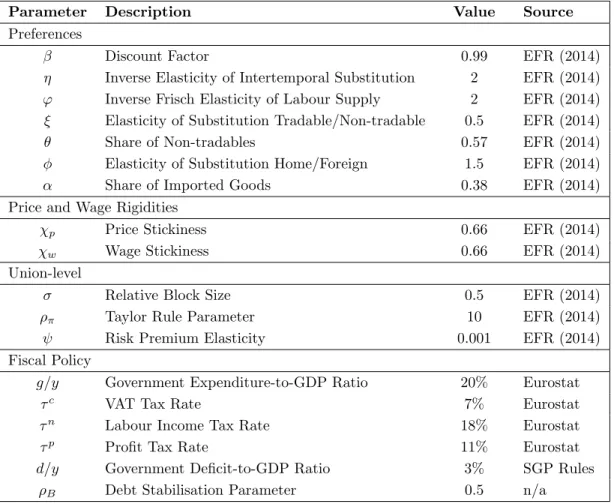
Parameter Description Value Source

Preferences

β Discount Factor 0.99 EFR (2014)

η Inverse Elasticity of Intertemporal Substitution 2 EFR (2014)

ϕ Inverse Frisch Elasticity of Labour Supply 2 EFR (2014)

ξ Elasticity of Substitution Tradable/Non-tradable 0.5 EFR (2014)

θ Share of Non-tradables 0.57 EFR (2014)

φ Elasticity of Substitution Home/Foreign 1.5 EFR (2014)

α Share of Imported Goods 0.38 EFR (2014)

Price and Wage Rigidities

χp Price Stickiness 0.66 EFR (2014)

χw Wage Stickiness 0.66 EFR (2014)

Union-level

σ Relative Block Size 0.5 EFR (2014)

ρπ Taylor Rule Parameter 10 EFR (2014)

ψ Risk Premium Elasticity 0.001 EFR (2014)

Fiscal Policy

g/y Government Expenditure-to-GDP Ratio 20% Eurostat

τc _{VAT Tax Rate 7% Eurostat}

τn _{Labour Income Tax Rate 18% Eurostat}

τp _{Profit Tax Rate 11% Eurostat}

d/y Government Deficit-to-GDP Ratio 3% SGP Rules

ρB Debt Stabilisation Parameter 0.5 n/a

Table 1: Parameter Values - Overview

determining preferences and nominal rigidities are taken directly from EFR, and are mostly standard values used in the literature. For the fiscal variables, values are calibrated to Euro-area averages over 1995-2015, taken from Eurostat data.9

Table 2 summarises the baseline calibration of the structural rigidities. The calibration strategy here also follows EFR. The tradable sector is taken to be the manufacturing sector and non-tradables are taken to be services. Due to the difficulty in measuring wage mark-ups, wage and price mark-ups are assumed to be equal in a given sector. The tradable sector mark-up in both blocks is set to 15%, in line with the average across both Core and Periphery Euro-area countries. The non-tradable sector mark-up in the Core block is set to 33%. The non-tradable sector of the Periphery block is assumed to face “excess” rigidities: here the initial elasticities are set to target a mark-up of 50%, in line with the estimated mark-up in Italy and Spain.

9_{The three tax rates are calibrated to match the revenue collected from each type of tax as a fraction of GDP. Specifically, the VAT} tax rate is set to target revenues from ‘taxes on products’ at 11% of GDP, the labour income tax rate is set to target revenues from ‘taxes on personal income’ and ‘household’s social contributions’ at 13% of GDP, and the profit tax rate is set to target the revenue from ‘taxes on profits and corporate income’ at 3% of GDP. This strategy implies tax rates lower than the statutory tax rates commonly used to calibrate models, for example in Vogel (2014). Conversely, using those tax rates would imply implausible revenue shares. Targeting the revenue shares is more appropriate, both because it directly gauges effective average tax rates, incorporating tax exemptions, tax evasion and distributional consequences of taxation, and more importantly because the revenue shares are of direct importance for the effects of structural reforms on total tax revenue.

Target Description Target Value Parameter

Tradable Sector Mark-up 1.15 T =γT = 7.7

Core Non-Tradable Sector Mark-up 1.33 ∗

N =γN∗ = 4

Periphery Non-Tradable Sector Mark-up 1.50 N =γN = 3

Table 2: Parameter Values - Structural RigiditiesSource: Eggertsson et al. (2014)

3.2

Results

In our model economy, imperfect competition in product markets leads to a mark-up of prices over marginal costs, and imperfect competition in labour markets leads to a mark-up of wages over the marginal disutility of labour. These mark-ups represent the distortions caused by regulations, and structural reforms will be defined as reductions in these mark-ups. We will label a reduction in price mark-ups as “Product Market Reform” (PMR), and a reduction in wage mark-ups as “Labour Market Reform” (LMR). Both of these reforms will boost output in the long run by removing distortions created by the excess regulations. In this model, reforms are supply-side expansions which can lead to lower inflation and declines in output in the short run. If the economy has inflation-targetting monetary policy, interest rates will fall in response to the decline in inflation, boosting demand and offsetting the decline in output. However, if monetary policy is unable to do this – for example if the country is in a currency union and so does not have flexible domestic monetary policy – then there is potential scope for expansionary fiscal policy to step in and provide the necessary boost in demand. In the results below, we will assume that monetary policy remains fixed throughout, and compare the cases with and without this fiscal stimulus. Note that these short run policies will not affect the long run impact of the reforms.

3.2.1 Long-run Effects of Reforms

To begin with, we look at the long run effects of reforms on to-GDP. Figure 1 shows the decline in the deficit-to-GDP ratio for different size reforms, measured here by the percentage reduction in mark-ups, showing separately the case of LMRs, PMRs and both together. Naturally, the deficit-to-GDP ratio falls more for larger reforms, and falls most when both reforms are carried out. However, it is clear that most of the gains in deficit-to-GDP come from the PMR, with even very large LMRs having only small effects. On the other hand, with LMRs and PMRs together, reducing the mark-ups by 15-16%, which would bring the Periphery countries in line with Core countries in the Euro-area, can cut the deficit-to-GDP ratio by a full percentage point. Nonetheless, for small reforms of either type, the gains are small. For example, with the baseline reform size of 1% considered in Sajedi (2018) and EFR, the long run gains in deficit-to-GDP are almost negligible.

3.2.2 Short-run Effects of Reforms

We now compare the short run costs of reforms under different fiscal policy scenarios. In all cases, we consider monetary policy to be fixed throughout the simulations. This means that in the first scenario we consider, No Stabilization, where fiscal policy remains fixed, there are short run output costs from the reform. Notice that these

Figure 1: Long Run Deficit-to-GDP Improvements from Reforms

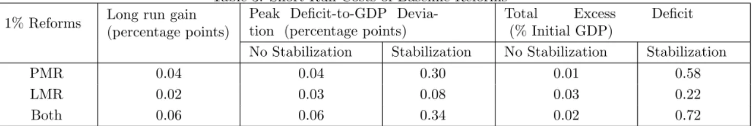
Table 3: Short Run Costs of Baseline Reforms

1% Reforms Long run gain

(percentage points)

Peak Deficit-to-GDP Devia-tion (percentage points)

Total Excess Deficit

(% Initial GDP)

No Stabilization Stabilization No Stabilization Stabilization

PMR 0.04 0.04 0.30 0.01 0.58

LMR 0.02 0.03 0.08 0.03 0.22

Both 0.06 0.06 0.34 0.02 0.72

costs of reform. Here, we will consider a fiscal policy rule that just fully offsets all the short run output costs from the reform. While output is stabilized in this scenario, there are additional fiscal costs due to the excess spending.

Baseline reforms under alternative fiscal policy scenarios

Table 3 shows the results of the baseline simulations. Again, we consider separately the case of LMRs, PMRs and both together. In each case, we report the long run gain in deficit-to-GDP, from Figure 1, which is independent of the short run fiscal policy scenario. We use two measures of the short run fiscal costs: the peak deviation of the deficit-to-GDP from its initial level, which captures the leeway required in fiscal rules that limit this ratio, and the total excess deficit within the transition, shown as a percentage of initial GDP, capturing the total dynamic fiscal cost.

As before we see that the majority of the long run gains in deficit-to-GDP come from the PMR, and that with the small baseline reform considered here, the effects are very small. In terms of the short run costs, we see that the fall

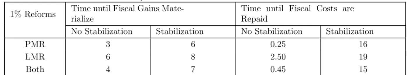
Table 4: Prompt Correction of Deficits under Baseline Reforms 1% Reforms Time until Fiscal Gains

Mate-rialize

Time until Fiscal Costs are Repaid

No Stabilization Stabilization No Stabilization Stabilization

PMR 3 6 0.25 16

LMR 6 8 2.50 19

Both 4 7 0.45 15

in output induces a fiscal cost during the reform, even absent any active fiscal stabilization. However, the effect is fairly small: we find a 0.03pp rise in deficit-to-GDP for the LMR, 0.04pp for the PMR and 0.06pp for both reforms together. The total excess deficit is very small, ranging from 0.01-0.03% of the initial GDP.

An active fiscal stimulus can offset the short run output costs of reform, but with an additional rise in the deficit. In particular, we find that the PMRs have the highest fiscal costs from active stabilization. In this case, the deficit-to-GDP can rise by 0.3pp, with a total fiscal cost of almost 0.6% of the initial GDP. In contrast, the LMRs require only a 0.08pp rise in deficit-to-GDP and a 0.22% total excess deficit to offset the short run output costs. While both reforms together have a higher overall cost, with a 0.34pp rise in deficit-to-GDP and 0.72% total excess deficit, it is worth noting that the cost is less than the sum of the costs of the individual reforms, suggesting complementarities between the reforms.

Gauging “prompt” correction of deficits

To capture whether the reforms lead to a “prompt” correction of deficits, we report two statistics in Table 4. First, we report the number of periods before the deficit-to-GDP falls below its initial level, in other words the time before the fiscal gains from the reform materialize. Second, we calculate the ratio of the total excess deficit to the long run gains from the reform, which captures the number of periods that it would take for the reduced deficit in the long run to repay the excess deficit in the short run. Again, we calculate these for different types of reform and under the alternative short run policy scenarios.

Looking first at the time for the fiscal gains to materialize, we see that without active stabilization it can still take between 9 and 18 months (3-6 quarters) for deficit-to-GDP to fall below its initial level. With active stabilization, this rises to 18-24 months (6-8 quarters). Despite the smaller fiscal cost, we see that the LMR takes the longest to provide any fiscal gains, but again the two reforms together can provide complementarities that make the fiscal gains materialize faster than the LMR alone.

Looking at the time to repay the total excess deficit with the long run fiscal gains from the reform, we see a similar pattern, with LMRs implying the longest time to repay. This is due to the fact that the long run gain are smaller for LMRs, meaning that even the smaller long run costs take longer to be repaid. Still, without active stabilization these numbers are small, with a maximum of 6-9months to repay the costs of the LMR. On the contrary, with active fiscal stabilization, these numbers are much larger. It can take 4-5 years (16-19 quarters) to repay the costs of either reforms alone, and still close to 4 years (15 quarters) to repay the cost of the reforms together.

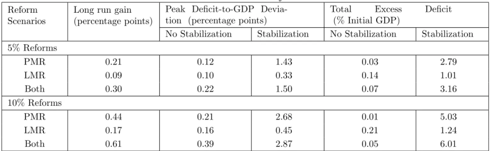
Table 5: Short Run Costs of Major Reforms Reform

Scenarios

Long run gain (percentage points)

Peak Deficit-to-GDP Devia-tion (percentage points)

Total Excess Deficit

(% Initial GDP)

No Stabilization Stabilization No Stabilization Stabilization

5% Reforms PMR 0.21 0.12 1.43 0.03 2.79 LMR 0.09 0.10 0.33 0.14 1.01 Both 0.30 0.22 1.50 0.07 3.16 10% Reforms PMR 0.44 0.21 2.68 0.01 5.03 LMR 0.17 0.16 0.45 0.21 1.24 Both 0.61 0.39 2.87 0.05 6.01

Defining “major” structural reforms

Finally, to gauge what should count as a “major” reform with significant fiscal implications, in Table 5 we compare the baseline reforms again two larger reforms of 5% and 10% reductions in mark-ups. Firstly, as seen earlier in Figure 1, the long run gains from the reforms increase almost exactly linearly with the rise in the size of the reform. For the most part the short run costs of reforms also increase with the size of the reform. The increase in the deficit-to-GDP that is implied by the larger reforms rises marginally in the case of no active stabilization, but increases almost linearly with the size of the reform in the case of the active stabilization. Even for the 5% reforms, there are now sizeable increases in the deficit-to-GDP of around 1.5pp implied by the PMRs and the joint reforms. For the 10% reforms, these numbers are even larger, between 2.5-3pp. The short run fiscal costs of the LMRs remains small, at 0.45pp even for the largest reforms. Similarly, in the case of the PMRs and joint reforms, the total excess deficit with active fiscal stabilization also grows with the size of the reforms, with around 3-6% excess deficit required to offset the short run output costs. However, the same is not true for LMRs, where the fiscal costs do not grow as quickly, and the total excess deficit remains around 1% of the initial GDP.

4

Combining Economic and Legal Analysis

The economic results inform the interpretation and application of the legal rules in several regards. First, the economic insight confirms the legal reasoning, though on a different methodological basis. The legal reasoning grounds flexibility on considerations related to discretionary power as well as the purpose and spirit of the norm, while the economic approach considers effects as derived through theoretical modeling. The economic analysis supports the leeway to account for the implementation of structural reforms identified through legal reasoning. Given the positive budgetary long-term effect of structural reforms, the legal rules should be applied with a degree of leniency allowing for a short-term deterioration of the fiscal position in return for greater long-term fiscal position. Second, the above applies not only to accepting the fiscal deterioration due to the immediate short-term contraction from structural reforms but also extends to fiscal stabilization. While active stabilization amplifies the fiscal deterioration in the short-term, it allows to return to the same post steady state fiscal position (and better than

the fiscal state without structural reforms being carried out) as in the scenario of no stabilization, i.e. strict enforcement of fiscal rules. Moreover, unlike under No Stabilization, if Active Stabilization is pursued the output losses associated with structural reforms are fully offset offering a desirable macroeconomic smoothing effect. In other words, leeway granted to the enforcement of fiscal rules comes at a considerable, but recoverable, fiscal costs in return for a significant macroeconomic benefit: On the one hand, short term fiscal costs for Active Stabilization is greater than in No Stabilization, but on the other hand, these fiscal costs unwind within a reasonable period of 6-8 quarters and, at the same time, provide a macroeonomic smoothing effect by offsetting output losses. From a legal perspective, this finding is compatible with the teleological interpretation of the fiscal rules, as mentioned above: Since the main purpose of the fiscal regimes lies in ensuring long-term fiscal compliance, infusing short-term flexibility to the legal rules is in line with this objective.

Third, the economic analysis suggests modifications to be made in light of the legal terms “prompt” (related to the timely positive budgetary effect). “Prompt” can be interpreted by reference to the “time to gains materialize” as calculated above. That is, the “time to repay”-concept offers a suitable tool to give meaning to the legal term “prompt”. Intuitively, “time to repay” is shorter in a scenario of fiscal leniency without a fiscal stabilization mechanism. However, within the scenarios above, even in the longest case (i.e. Active Stabilization) these gains materialize within 2 years and the fiscal costs are entirely repaid in 4-5 years, which can be considered not to be overly long.

Fourth, the “major”-requirement attached to the size of structural reforms can be determined on basis of the economic analysis. In principle, excluding minor structural reforms from being eligible for fiscal leeniency does not seem compatible with the linear relationship of short-term costs and long-term benefits across different sizes of structural reforms. That is, minor structural reforms also produce higher benefits than costs and should generally be accepted. Also, while larger reforms typically produce larger absolute benefits and should thus be preferable over small size reforms, they also require proportionally more fiscal leeniency in the short run. Finally, the economic analysis further refines our understanding on the type of structural reform which should be implemented. PMR tend to produce larger deficit-reducing effects than LMR and should, from this perspective, be preferred. Also, there is an indication that a combination of both PMR and LMR offer fiscal advantages, as the total excess deficit is less than the sum of the individual reforms, suggesting complementarities between the reforms. Hence, the legal term “major”, from a perspective of teleological interpretation, should not only be indifferent for the size of the reform but also account for the type of reform to be pursued.

5

Conclusions

The EU debt crisis has revealed tensions between legal and economic reasoning. Most prominently, interpretation of the legal provisions stipulating a prohibition to bailout sovereign states as well as the ban on monetary financing gave rise to different approaches in legal and economic reasoning when adopted in disciplinary isolation (De Grauwe et al. 2017). Another, yet unexplored, field of analysis are legal and economic approaches to the interpretation of fiscal rules. Interaction of legal and economic analysis becomes particularly interesting where the effect of structural reforms is concerned. Reforms are generally desirable within an economic union, as they offer positive spillovers for

reconciled – this analysis has offered the economic underpinning necessary to sustain economically sound legal interpretation of EU fiscal governance rules. Given the nature and size of the positive fiscal long-term effects, there is a strong indication towards employing an interpretation of fiscal rules in light of these effects. Hence, the analysis rejects a rigid application of fiscal rules ignoring the effects of structural reforms in the long-term. Rather, there is scope for a “stick-and-carrot”-application of fiscal rules rendering structural reforms a suitable incentivizing device for fiscal leeway (and thus sparing the country from sanctions for rule violation).

The results may further inform the ongoing debate on reforming EU economic surveillance. Recent policy proposals have stressed the importance of structural reforms and pointed at the use of existing instruments in implementing structural reforms (Juncker 2015). We have offered intuition for designing fiscal rules in a way that permits to account for the effect of structural reforms. On a more general note, our analysis calls for a coordination of economic policies recognizing the interdependent nature of fiscal policy and structural economic policies. Future institutional arrangements should reflect that enforcement of fiscal adherence should not be pursued as short-term objective per se but rather incorporate the positive long-term fiscal effects associated with sound structural policies.

References

Antonakakis, N. and Vergos, K.: 2013, Sovereign bond yield spillovers in the euro zone during the financial and debt crisis,Journal of International Financial Markets, Institutions and Money26(C), 258–272.

Beetsma, R. and Debrun, X.: 2004, Reconciling Stability and Growth: Smart Pacts and Structural Reforms,IMF

Staff Papers51(3), 431–456.

Borger, V.: 2016, Outright monetary transactions and the stability mandate of the ecb: Gauweiler,Common Market

Law Review53, 139–196.

Calvo, G. A.: 1983, Staggered Prices in a Utility-Maximizing Framework, Journal of Monetary Economics

12(3), 383–398.

De Grauwe, P.: 2016,Economics of Monetary Union, OUP Catalogue, 11 edn, Oxford University Press.

De Grauwe, P., Ji, Y. and Steinbach, A.: 2017, The EU debt crisis: Testing and revisiting conventional legal doctrine,International Review of Law and Economics51, 29 – 37.

Eggertsson, G., Ferrero, A. and Raffo, A.: 2014, Can Structural Reforms Help Europe?, Journal of Monetary

Economics61(C), 2–22.

European Commission, .: 1997a, Article 2, Regulation (EC) no. 1467/97. European Commission, .: 1997b, Article 5, Regulation (EC) no. 1466/97. European Commission, .: 2014, Quarterly Report on the Euro Area.

European Commission, .: 2015a, Annual Growth Survey 2015, Communication COM (2014) 902.

European Commission, .: 2015b, Making the Best Use of the Flexibility Within the Existing Rules of the SGP, Communication COM (2015) 12 final.

Fat´as, A. and Mihov, I.: 2010, The Euro and Fiscal Policy,Europe and the Euro, NBER Chapters, National Bureau of Economic Research, Inc, pp. 287–324.

Fiori, G., Nicoletti, G., Scarpetta, S. and Schiantarelli, F.: 2012, Employment effects of product and labour market reforms: Are there synergies?,The Economic Journal122(558), F79–F104.

Griffith, R. and Harrison, R.: 2004, The Link Between Product Market Reform and Macro-Economic Performance,

European Commission European Economy - Economic Papers 209, Directorate General Economic and Financial

Affairs (DG ECFIN).

Griffith, R., Harrison, R. and Macartney, G.: 2007, Product market reforms, labour market institutions and unemployment,The Economic Journal117(519), C142–C166.

International Monetary Fund, .: 2017, Structural Reforms in the Euro Zone: an IMF Perspective, Speech by Paul Thomsen, director of the IMF’s European Department at the European Central Bank conference Structural reforms in the euro area.

Juncker, J.: 2015, Completing Europe’s Economic and Monetary Union, Five Presidents’ Report.

https://ec.europa.eu/priorities/sites/beta-political/files/5-presidents-report en.pdf.

Lenaerts, K. and Guti´errez-Fons, J. A.: 2014, To say what the law of the eu is: Methods of interpretation and the european court of justice,Columbia Journal of European Law20, 3 – 61.

Mourougane, A., Botev, J., Fournier, J.-M., Pain, N. and Rusticelli, E.: 2016, Can an increase in public investment sustainably lift economic growth?,OECD Economics Department Working Papers(1351).

Palmstorfer, R.: 2012, To bail out or not to bail out? the current framework of financial assistance for euro area member states measured against the requirements of eu primary law,European Law Review37, 771.

Panizza, U. and Presbitero, A. F.: 2014, Public debt and economic growth: Is there a causal effect?, Journal of

Macroeconomics41, 21 – 41.

Poplawski Ribeiro, M. and Beetsma, R.: 2008, The Political Economy of Structural Reforms Under a Deficit Restriction,Journal of Macroeconomics30(1), 179–198.

Sajedi, R.: 2018, Fiscal consequences of structural reform under constrained monetary policy,Journal of Economic

Dynamics and Control.

Steinbach, A.: 2013, Economic policy coordination in the euro area.

Vogel, L.: 2014, Structural Reforms at the Zero Bound, European Commission European Economy - Economic