Independent Effects of Reynolds and Mach Numbers on the
Aerodynamics of an Iced Swept Wing
Andy P. Broeren1
NASA John H. Glenn Research Center, Cleveland, Ohio, 44135 USA
Sam Lee2
Vantage Partners, LLC, Cleveland, Ohio, 44135 USA
Brian S. Woodard3
University of Illinois at Urbana-Champaign, Urbana, Illinois, 61801 USA
Christopher W. Lum4
University of Washington, Seattle, Washington, 98195 USA
Timothy G. Smith5
FAA William J. Hughes Technical Center, Atlantic City Airport, New Jersey, 08405 USA Aerodynamic assessment of icing effects on swept wings is an important component of a larger effort to improve three-dimensional icing simulation capabilities. An understanding of ice-shape geometric fidelity and Reynolds and Mach number effects on the iced-wing aerodynamics is needed to guide the development and validation of ice-accretion simulation tools. To this end, wind-tunnel testing was carried out for a 13.3%-scale semispan wing based upon the Common Research Model airplane configuration. The wind-tunnel testing was conducted at the ONERA F1 pressurized wind tunnel with Reynolds numbers of 1.6×10⁶ to 11.9×10⁶ and Mach numbers of 0.09 to 0.34. Five different configurations were investigated using fully 3D, high-fidelity artificial ice shapes that maintain nearly all of the 3D ice accretion features documented in prior icing-wind tunnel tests. These large, leading-edge ice shapes were nominally based upon airplane holding in icing conditions scenarios. For three of these configurations, lower-fidelity simulations were also built and tested. The results presented in this paper show that while Reynolds and Mach number effects are important for quantifying the clean-wing performance, there is very little to no effect for an iced-wing with 3D, high-fidelity artificial ice shapes or 3D smooth ice shapes with grit roughness. These conclusions are consistent with the large volume of past research on iced-airfoils. However, some differences were also noted for the associated stalling angle of the iced swept wing and for various lower-fidelity versions of the leading-edge ice accretion. More research is planned to further investigate the key features of ice accretion geometry that must be simulated in lower-fidelity versions in order to capture the essential aerodynamics.
1 Research Aerospace Engineer, Icing Branch, 21000 Brookpark Rd., MS 11-2, Associate Fellow AIAA. 2 Engineer V, Icing Branch, 21000 Brookpark Rd., MS 11-2, Senior Member AIAA
3 Research Associate, Dept. of Aerospace Engineering, 306 Talbot Lab, 104 S. Wright St., Member AIAA. 4 Research Assistant Professor, William E. Boeing Department of Aeronautics and Astronautics, Guggenheim Hall Room 211, Box 352400, Member AIAA.
5 Engineer, Aircraft Icing Research Program, ANG-E282, Bldg. 210.
I. Nomenclature
b = wing span
c = local streamwise chord length
CD = drag coefficient
CD,min = minimum drag coefficient
CD,0.6 = drag coefficient at CL = 0.6.
CL = lift coefficient
CL,max = maximum lift coefficient
CL,use = usable lift coefficient
CM = quarter-chord mean aerodynamic chord pitching moment
CM,min = minimum quarter-chord mean aerodynamic chord pitching moment
Cp = model surface pressure coefficient
LWC = icing cloud liquid water content
M = freestream Mach number
MAC = mean aerodynamic chord
MCCS = maximum combined cross section
MVD = median volumetric diameter of icing cloud drop distribution
po = freestream total pressure
q = freestream dynamic pressure
Re = freestream Reynolds number based on mean aerodynamic chord RLE = removable leading edge
Vs,1g = aircraft 1-g stall speed
x = wing streamwise coordinate
y = wing spanwise coordinate
z = wing thickness coordinate
α = model angle of attack
αstall = stalling angle of attack, consistent with the maximum lift coefficient
αuse = usable angle of attack, consistent with the usable lift coefficient
II. Introduction
Ice accretion and the resulting aerodynamic effect on large-scale swept wings is an extremely complex problem that affects the design, certification and safe operation of transport airplanes. Broeren et al.1 describe the current situation where there is increasing demand to balance trade-offs in aircraft efficiency, cost and noise that tend to compete directly with allowable performance degradations over a large range of icing conditions. These trade-offs, combined with the ever-present demand to reduce development cost, requires an increased reliance on computational tool development. In addition, NASA is conducting research toward future generations of advanced airplane configurations with ambitious goals to improve efficiency while reducing emissions and noise. This research also relies on the development of advanced icing simulation tools in order to realize these design goals. However, sufficient high-quality data to evaluate the performance of these icing simulation tools on iced swept wings are not currently available in the public domain. This problem is being addressed through a large collaborative research effort sponsored by NASA, the Office National d’Etudes et Recherches Aérospatiales (ONERA) and the Federal Aviation Administration (FAA).
A main objective of this collaborative research effort was accomplished in the year 2016 with the publication of an experimental ice-accretion database for large-scale swept wings.2 A primary purpose of this database is for the evaluation of three-dimensional icing simulation tools such as those being developed within NASA and ONERA.3,4 There is an inherent difficulty as to how these comparisons should be conducted because of the large-scale, three-dimensionality associated with the experimental ice accretion in some cases (e.g., “scallops” or “lobster tails”). Furthermore, most icing simulations tools are not capable of predicting these large-scale, three-dimensional ice features. An important question is how much detail of this three-dimensional geometry is critical to the iced-wing aerodynamics and therefore must be accurately simulated. One possible comparison metric is the resulting potential aerodynamic degradation of the swept-wing. Therefore, the remaining objectives of the larger, collaborative research effort are to:
Develop a systematic understanding of the aerodynamic effect of icing on swept wings including: Reynolds and Mach number effects, important flowfield physics and fundamental differences from 2-D.
Determine the level of ice-shape geometric fidelity required for accurate aerodynamic simulation of swept-wing icing effects.
This paper, along with a series of companion papers,5-7 provides initial results for these remaining objectives. Additional wind-tunnel testing and future publications are planned. The approach used to accomplish these objectives has been successfully carried out in previous icing aerodynamics studies of straight wings and airfoils.
In past work, geometric representations of ice accretion have been attached to wings and models and tested in dry-air wind tunnels or in flight. These geometric representations are known as “artificial ice shapes” or “ice-accretion simulations.” The various methods and geometric fidelities associated with developing artificial ice shapes have been investigated in a previous NASA-ONERA collaborative research effort called “SUNSET1.”8 Since that time, a new approach for producing high-fidelity artificial ice shapes have been developed using 3-D scanning and rapid-prototype manufacturing (RPM).9 In past studies of icing performance effects on airfoils, systematic investigations of Reynolds and Mach number effects were conducted.10-16 Over the course of many years, it was found that aerodynamic tests conducted in the Reynolds number range of 1.0 to 2.0×10⁶ could yield results applicable to flight Reynolds number (e.g., 10 to 20×106) for leading-edge ice shapes. Therefore, the current research effort will determine if similar trends apply for full-span, leading-edge ice on a swept wing. This effort involves both low- and high-Reynolds number aerodynamic testing. The low-Reynolds number aerodynamic testing is being conducted in the Wichita State University (WSU) 7-ft x10-ft size atmospheric wind tunnel. The high-Reynolds number aerodynamic testing is being conducted in the ONERA F1 11.4-ft x 14.8-ft pressurized wind tunnel using a larger scale model. The pressurization capability of this facility will allow for independent variations in Reynolds number up to approximately 12×106 and Mach number up to approximately 0.34. The results from the ONERA F1 test campaigns will be analyzed for Reynolds and Mach number effects (among other things) and compared to the results of the WSU test campaigns to determine the extent to which iced, swept-wing aerodynamic testing can be conducted in smaller-scale facilities at lower Reynolds number.
The purpose of this paper is to present the results of the high-Reynolds number testing with the objective of quantifying the effects of Reynolds and Mach number on clean- and iced-wing performance over the range tested. In order to carry out this objective, aerodynamic testing was conducted at the ONERA F1 wind tunnel using a 13.3% scale semispan wing model of the CRM65. The CRM65 geometry is based upon the Common Research Model described in previous papers1,17-20 and in Section II.B. Clean, tripped and iced-wing configurations were tested. The artificial ice shapes were based upon 3-D scans of ice accretion in the NASA Icing Research Tunnel (IRT) and fabricated with rapid-prototype manufacturing. The resulting artificial ice shapes were also instrumented to measure surface static pressure. Aerodynamic performance testing was conducted in angle of attack sweeps over a Reynolds number range of 1.6×10⁶ to 11.9×10⁶ and a Mach number range of 0.09 to 0.34. Force balance and surface pressure data were acquired. Mini-tuft flow visualization was also performed during the performance sweeps. The companion papers by Lee et al.,5 Woodard et al.6 and Sandhu et al.7 provide more results regarding the effect of artificial ice shapes on the wing aerodynamic performance and flowfield.
III. Wind-Tunnel Facility, Model and Experimental Methods
A. Wind-Tunnel Facility
All experiments discussed in this paper were carried out at the ONERA F1 pressurized wind tunnel located at the Fauga-Mauzac Center in southern France. The closed-return tunnel can be pressurized to 56 psi and has a test section approximately 11.5-ft high x 14.8-ft wide. The maximum speed is M = 0.36 at a pressure of approximately 22 psi which corresponds to a Reynolds number per foot of approximately 3.7×10⁶. The maximum Reynolds number is 6.1×10⁶/ft at a pressure of approximately 56 psi and M = 0.23. During an experiment the Mach number was controlled to within ±0.001 while the total pressure and total temperature were controlled to within ±0.03 psi and ±0.4 °F, respectively. The angle of attack sweeps were performed with a continuous change in pitch angle at a constant rate of 0.1 deg/sec. The model angle of attack was varied from -6 deg up to 25 deg except in cases where dynamic forces limited the maximum angle of attack or a clear local maximum in lift coefficient was measured. Force balance and surface pressure measurements were acquired for most configurations at Reynolds and Mach number combinations shown in Table 1 along with the approximate values of total pressure (po) and dynamic
pressure (q∞). For some configurations, some of these conditions were omitted in order to optimize the efficiency of the test campaign. The speed control was based upon Mach number, therefore small differences in Reynolds number were observed. For example, the Reynolds number corresponding to M = 0.23 varied between 11.8×10⁶ and 12.0×10⁶. Torz-Dupuis21 has provided a detailed report of the test set-up and instrumentation, data reduction, experimental uncertainties and wall corrections.
Table 1. Reynolds and Mach Number Conditions
Reynolds Number
Mach Number
0.09 0.18 0.23 0.27 0.34 1.6×10⁶ pq o = 18.9 psi = 0.10 psi
2.7×10⁶ pq o = 30.5 psi = 0.17 psi pq o = 16.0 psi = 0.35 psi
4.0×10⁶ pq o = 46.4 psi = 0.26 psi pq o = 23.2 psi = 0.52 psi pq o = 18.9 psi = 0.65 psi pq o = 16.0 psi = 0.78 psi
6.8×10⁶ pq o = 39.2 psi = 0.88 psi pq o = 31.9 psi = 1.1 psi pq o = 27.6 psi = 1.3 psi pq o = 21.8 psi = 1.7 psi 9.6×10⁶ pq o = 55.1 psi = 1.2 psi
11.9×10⁶ pq o = 55.1 psi = 2.0 psi
Load measurements were performed using a 6-component force balance located beneath the test section floor. This study utilized a reflection plane model and the force balance was used to measure the lift, drag and pitching moment. The force balance does not directly measure the lift and drag but rather it measures the normal force and the axial force which are relative to a coordinate system fixed to the force balance. A coordinate transformation is required to determine the lift and drag in the wind axes. The force balance measures the moment about a reference point fixed to the force balance and it is necessary to transfer the moment to the reference point on the model. For the model used in this study there was an offset along the x-axis of the force balance between the balance reference point and the model reference point. The model center of rotation and moment center are defined below in Section II.B. In general, the uncertainty of each force balance component was ±0.04% to 0.06% of the capacity. The measurement uncertainty in the wing angle of attack was ±0.023 deg. Specific uncertainty values for the wing forces and pitching moment are described later in this section.
Surface pressure measurements were acquired using miniature electronic pressure scanning (ESP) modules developed by Pressure Systems. A total of six 64-channel ESP modules were used each having a full-scale measurement range of ±15.0 psi. The pressure data acquisition system at F1 is designed to accommodate the changes in tunnel stagnation pressure for the various run conditions through changes in the reference pressure. The system ensures that the fullest range of the ESP modules is utilized without exceeding the measurement limit. Specific uncertainty values for model pressure coefficient are described later in this section. The wind-tunnel reference pressures are measured on individual Druck transducers. The resulting uncertainty in the dynamic pressure is an approximately linear function of the magnitude of the dynamic pressure and ranges from ±8.65% at the Re = 1.6×10⁶, M = 0.09 (lowest dynamic pressure) condition to ±0.46% at the Re = 12.0×10⁶, M = 0.23 (highest dynamic pressure) condition. This large range of uncertainty in dynamic pressure reflects the challenges of providing instrumentation for a pressurized wind tunnel where there is a correspondingly large range of pressures and forces to be measured.
The uncertainties in the experimental data were determined using the standard “root-sum-square” (RSS) method outlined by Coleman and Steele22 and developed by Kline and McClintock.23 These uncertainties are estimated for 20:1 odds and use the numerical values for the instrumentation described in the preceding paragraphs. Table 2 provides a summary of the absolute and relative uncertainties the model surface pressure coefficient for the lowest and highest dynamic pressure. The uncertainties for other Reynolds and Mach number conditions follows an approximately linear relationship with the corresponding dynamic pressure shown in Table 1. The data show that for pressure coefficients of about -5 or less, nearly all of the uncertainty is due to the dynamic pressure itself. For example, the uncertainty in dynamic pressure for Re = 1.6×10⁶, M = 0.09 is ±8.65% while the uncertainty in the pressure coefficient is ±8.79% meaning 99% of the total uncertainty is due to the uncertainty in dynamic pressure. Table 3 provides a summary of the uncertainties in lift, drag and pitching moment coefficient for the lowest and highest dynamic pressure for the clean-wing configuration. For the lowest dynamic pressure at Re = 1.6×10⁶ and M = 0.09, the uncertainty values are large, especially for the drag and pitching-moment coefficients. The large
uncertainties reported in Table 3 are due to low magnitude of the measured force and moment on the force balance. It is important to note that the force-balance uncertainties were reported based upon the maximum forces and moments for the current test. Therefore, the total uncertainties reported in Table 3 would likely be much smaller if the force-balance uncertainties were provided over the smaller range associated with the lowest dynamic pressure. In other words, the actual uncertainties in lift, drag and pitching-moment coefficient for the lowest dynamic pressure are likely much lower than the values reported in Table 3. Lee et al.5 provide further justification for this conclusion by comparison of the data acquired on the 8.9% scale model at the WSU wind tunnel. For the highest dynamic pressure at Re = 11.9×10⁶, M = 0.23, all of the uncertainty values are much more reasonable and acceptable for the purposes of this work.
Table 2. Absolute and Relative Uncertainties in Model Surface Pressure Coefficient
Pressure Coefficient Absolute Uncertainty Relative Uncertainty
Re = 1.6×10⁶,
M = 0.09 ±1 ±0.116 -5 ±0.440 ±11.57% ±8.79%
Re = 11.9×10⁶,
M = 0.23 ±1 ±0.006 -5 ±0.023 ±0.62% ±0.46%
Table 3. Absolute and Relative Uncertainties in Force Balance Data
Variable Reference Value Uncertainty Absolute Uncertainty Relative
Re = 1.6×10⁶, M = 0.09 α 4.99 deg ±0.023 deg ±0.46% CL 0.5607 ±0.0530 ±9.45% CD 0.0203 ±0.0115 ±56.78% CM -0.2298 ±0.0273 ±11.86% Re = 11.9×10⁶, M = 0.23 α 4.97 deg ±0.023 deg ±0.46% CL 0.5951 ±0.0038 ±0.63% CD 0.0186 ±0.0007 ±3.55% CM -0.2363 ±0.0023 ±0.96%
The force balance and surface pressure measurements were synchronized in time within the facility data acquisition system. This was important since the data were acquired as the model was pitched continuously at a rate of 0.1 deg/sec. A custom-designed, post-processing routine was written and implemented for these data to conditionally average the results into 0.5 deg angle of attack increments using a ±0.15 deg window based upon the geometric (uncorrected) angle of attack. For example, data acquired over the interval 3.85 deg ≤α≤ 4.15 deg were used to create conditionally averaged values for α = 4 deg. In addition to this, the pitching-moment coefficient referenced to quarter-chord of the mean aerodynamic chord was also calculated. In previous reports and papers,24-26 the pitching moment was referenced to the location described below in Section II.B. After conducting further analysis of the data, a determination was made to report the pitching moment about the quarter-chord of the mean aerodynamic chord location that is also described in Section II.B.
All aerodynamic data (α, CL, CM, CD and Cp) presented in this paper were corrected for wind-tunnel-wall effects
using a linearized compressible flow method that models the potential flow around the model and wind-tunnel walls. This was an in-house ONERA method that yielded two corrections terms, one of which was constant and the other proportional to the model lift coefficient. The corrections were performed in real-time as the data were being acquired, however, the raw data are archived in the event of new post-processing requirements. In addition to this method a correction procedure for 3D models outlined in Barlow et al.27 as implemented by WSU28 was also used for comparison. The model and wind-tunnel constants used in this method were updated from the WSU-related values to those of the F1 model and wind tunnel. As described in Section I, aerodynamic data acquired at the WSU
wind tunnel will be compared with data acquired at the ONERA F1 facility. Therefore, it is important that the effect of the wind-tunnel walls on the aerodynamic data from both facilities be accounted for properly. The companion paper by Lee et al.5 provides comparison and analysis of the results of the wall correction schemes. The aerodynamic data reported in this paper were corrected using the ONERA method.
B. Wind-Tunnel Model Description
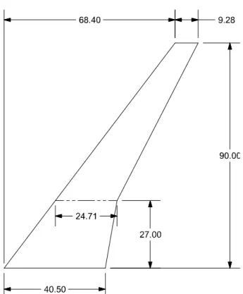
The semispan model fabricated for these wind-tunnel tests was based on a 13.3% scale version of the CRM65 wing. The full-scale CRM65 geometry has a realistic cruise configuration loading applied to the wing resulting in a wing shear similar to dihedral.17 In order to simplify the design of the removable leading edge segments (described below), this shearing or “bending” of the wing was removed from the model geometry resulting in an unsheared wing with a straight leading edge across the span of the model. The wing retained the twist and taper of the CRM65. Table 4 summarizes the geometric parameters of the wing, and a diagram of the CRM planform is shown in Fig. 1 with key dimensions. The main body of the model was machined from stainless steel while the removable leading edge components were machined from aluminum. The model contained 243 pressure taps in its clean configuration. Figure 2 shows photographs of the wing model installed in the wind tunnel with the circular splitter plate. An artificial ice shape is mounted to the leading edge of the wing in these images. Below the circular splitter plate was a streamlined shroud that covered the wing spar. This arrangement isolated the wing spar from any aerodynamic loads. With this arrangement both the splitter plate and shroud were non-metric meaning the aerodynamic forces were only measured on the wing itself. The splitter plate and shroud were designed based upon previous work for the smaller scale WSU wind-tunnel model.24,26
Table 4. Summary of 13.3% Scale CRM65 Semispan Wing Geometric Parameters
Wing Parameter Value
Span, b 7.5 ft (90.00 inches) MAC 2.08 ft (25.01 inches) Area (Geometric) 13.55 ft2 (1951.0 in2) Volume 2.09 ft3 (3604.5 in3) Aspect ratio† 8.3 Taper ratio 0.23
Root chord 3.38 ft (40.50 inches)
Tip chord 0.77 ft (9.28 inches)
Root α 4.4 deg.
Tip α -3.8 deg.
1/4-chord sweep angle 35 deg. Leading edge sweep angle 37.2 deg.
Location of rotation center‡ x = 29.05 in., z = 0 Location of moment center‡ x = 35.80 in., z = 0 Location of 0.25×MAC‡ x = 26.23 in., z = 0
†--While the other parameters in this table are defined specifically for this model, the aspect ratio is defined for a complete airplane configuration using the formula, .
‡--(0, 0, 0) is the wing root-section leading edge at zero angle of attack.
Figure 2. Photographs of 13.3% scale CRM65 semispan wing installed in ONERA F1 test section; left image shows wing lower surface, right image shows wing upper surface.
The model was designed and built with a removable leading edge that allowed artificial ice-shapes to be added to the wing. This approach has been used in previous icing aerodynamic studies8,11,13,15,16 and allows for very efficient and repeatable changes in the artificial ice-shape configurations. This is important for this research effort, since many different ice-shape configurations were investigated. The main components of the model were: the main element (including a spar that attached to the force balance); a full-span clean leading edge; and a partial-span leading edge used for mounting ice shapes. An open channel exists between the main element and any of the leading edge components for routing pressure tubing out the base of the model to the data acquisition system. The seam between the clean leading edge and the main element was a straight line on both the upper and lower surfaces, but the seam was not at the same location on both surfaces. Typically, ice accretes farther back on the wing of an aircraft on the lower surface than the upper surface, so the lower surface artificial ice shapes cover a greater portion of the local chord. At the root of the wing, the seam was at 9.3% and 22.9% of the local streamwise chord on the upper and lower surfaces, respectively. At the tip of the wing, the seam was at 12.6% and 38.4% of the local streamwise chord on the upper and lower surfaces, respectively.
The span removable leading edge was used to mount the artificial ice shapes to the wing. The partial-span removable leading edge extended from the root to 83.3% of the semipartial-span, and it contained a portion of the airfoil contour on the lower surface. Artificial ice shapes were attached to this removable leading edge and covered the entire upper surface of this removable leading edge. No pressure taps were added to this leading edge. Outboard of this partial-span leading edge, the artificial ice shapes were attached directly to the main element. The reason for this is that the model thickness decreases significantly on the outboard portion of the wing. There was not enough material to extend the removable leading edge. This design does not adversely affect the efficiency or repeatability of the artificial ice-shape configuration changes. The artificial ice shapes were created using a rapid prototype manufacturing (RPM) technique called stereo-lithography (SLA). The SLA process utilizes an ultraviolet laser to solidify liquid polymer resins, and the specific polymer chosen for these components was Accura 60. Tolerances are advertised to be about +/- 0.005 inches for this process. A representative ice shape was added to the wing geometry for each segment of wing span. The leading edge was divided into three segments that were approximately 37.8 in long. Pressure taps were installed in each of these segments at the same locations as on the clean removable leading edge. The pressure tap holes were included in the RPM design, and then stainless steel tubes were glued into each hole and plumbed to the quick disconnect.
The 243 pressure taps in the model were distributed in seven different streamwise rows. The tap rows were identified by the spanwise location. Further information regarding each of the tap rows can be found in Table 5 and the tap row locations are shown graphically in Fig. 3. Tap rows 1 through 6 each contained upper and lower surface taps as well as a tap located at the leading edge of that row. There were no lower-surface taps in row 7 because the wing section was too thin at this location. The taps in the main element of the model were plumbed with stainless steel tubing from their location on the surface out the root of the model. The taps in the leading edge required a more complicated route. The stainless steel tubing in both the clean leading edge and in the RPM ice leading edges transitioned to plastic tubing and then connected to a Scanivalve quick disconnect fitting. The use of these fittings allowed relatively quick model reconfigurations between clean and RPM leading edges.
Figure 3. Pressure tap row locations on the wing model. Upper Surface
Table 5. Details of the Pressure Tap Instrumentation
Row Identifier
Spanwise Location
y/b inches Taps in RLE Surface Upper Surface Lower Total Taps
1 0.111 10.0 20 13 5 38 2 0.278 25.0 22 12 4 38 3 0.444 40.0 22 12 4 38 4 0.600 54.0 22 12 4 38 5 0.705 63.5 22 12 4 38 6 0.811 73.0 22 12 4 38 7 0.900 81.0 7 8 0 15
C. Boundary-Layer Trip Configurations
The model was tested with boundary-layer trips applied near the leading edge on both upper and lower surfaces of the wing. The trips consisted of CADCUT trip dots which is an off-the-shelf product available in discrete sizes. The trip height was scaled by a factor of 1.5 from the height used in the previous testing with the 8.9% scale CRM65 wing model at WSU based upon the Reynolds number of 1.6×10⁶. The resulting trip heights on the F1 model were 0.0031 in (CADCUT P/N 3.1) and 0.0114 in (CADCUT P/N 11.4) on the upper and lower surface, respectively. The lower-surface trip location was determined by measuring the surface length from the leading-edge hilite in a direction perpendicular to the leading edge. At tap rows 1, 4 and 6, these distances were 3.00, 2.06 and 1.82 in, respectively. This lower-surface trip location was consistent with the 8.9% scale model. The upper-surface trip was located between 2.5% and 3.0% of the local streamwise chord. This location was selected so that the trip was downstream of the leading edge suction peak for most angles of attack. It should be noted that this location was farther downstream than the location used during the 8.9% scale model tests at WSU. Since this location was different, an additional set of runs were performed with the upper-surface trip located very close to the leading-edge hilite consistent with the trip configuration on the 8.9% scale model.
D. Artificial Ice-Shape Configurations
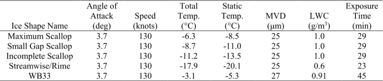
In addition to the clean aluminum machined leading edge, several other leading-edge configurations were tested. Numerous artificial ice shapes have been developed for aerodynamic testing and are summarized by Camello et al.25 for the 8.9% scale CRM65 wing tested at WSU. Selected configurations were also tested at F1 on the 13.3% scale model. Table 6 provides a summary of these selected configurations and the corresponding nominal icing conditions. Ice accretion testing was performed on three individual sections of the full-scale CRM65 reference wing: one taken at y/b = 0.20 called the Inboard model; one taken at y/b = 0.64 called the Midspan model; and one taken at y/b = 0.83 called the Outboard model. Broeren et al.,2 provide more details regarding the ice-accretion testing. The ice shapes were generated based upon an airplane angle of attack of 3.7 deg. The icing conditions were nominally based upon a CRM65 airplane in holding conditions in the United States Code of Federal Regulations, Title 14, Part 25, Appendix C, Continuous Maximum (hereafter: App. C). The Streamwise/Rime and WB33 ice shapes were directly scaled from App. C to the airspeed of 130 knots. The other conditions were not directly scaled from App. C, but instead represent a range in air temperature with the other conditions fixed. The ice-accretion testing was performed in the NASA Icing Research Tunnel and the ice geometry was measured using the 3D laser scanning method.9
Table 6. Summary of Icing Conditions for F1 Test Campaign Artificial Ice Shapes
Ice Shape Name
Angle of Attack
(deg) (knots) Speed
Total Temp. (°C) Static Temp. (°C) MVD (μm) (g/mLWC 3) Exposure Time (min) Maximum Scallop 3.7 130 -6.3 -8.5 25 1.0 29
Small Gap Scallop 3.7 130 -8.7 -11.0 25 1.0 29
Incomplete Scallop 3.7 130 -11.2 -13.5 25 1.0 29
Streamwise/Rime 3.7 130 -17.9 -20.1 25 0.6 23
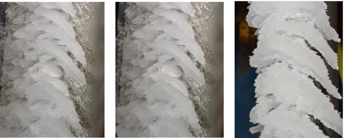
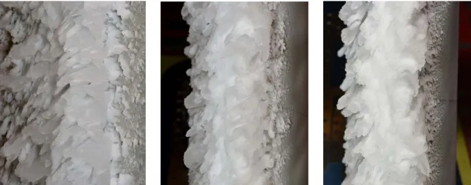
Figures 4-8 show photographs of the ice accretion on each of the three models (Inboard, Midspan and Outboard). The “Maximum Scallop” configuration (Fig. 4) was so named because of the well-defined scallop (or “lobster tail”) ice geometry that is clearly shown in the photographs for each model. Decreasing the total temperature 2.4 °C significantly changed the morphology of the scallop geometry as shown in Fig. 5. The size, orientation (angle of scallop) and gap between the scallops were all significantly altered and the ice shape was thus named “Small Gap Scallop.” Decreasing the total temperature another 2.5 °C caused the scallop gaps to close, leaving only some scallop tips at the chordwise extremities of each ice accretion (Fig. 6) and the ice shape was thus named “Incomplete Scallop.” The Streamwise/Rime shape shown in Fig. 7 was characterized by large-scale rime feathers, particularly on the Inboard model. The ice on the Midspan and Outboard models was characterized by a main ice shape formed at the attachment line with rime feathers downstream. Finally, the WB33 ice shape shown in Fig. 8 was characterized by highly three-dimensional ice features, some of which resembled scallop tips. The name “WB33” was derived from the specific flight condition associated with this case.2
Figure 4. Photographs of Maximum Scallop ice shape on Inboard (left), Midspan (middle) and Outboard (right) models.
Figure 5. Photographs of Small Gap Scallop ice shape on Inboard (left), Midspan (middle) and Outboard (right) models.
Figure 6. Photographs of Incomplete Scallop ice shape on Inboard (left), Midspan (middle) and Outboard (right) models.
Figure 7. Photographs of Streamwise/Rime ice shape on Inboard (left), Midspan (middle) and Outboard (right) models.
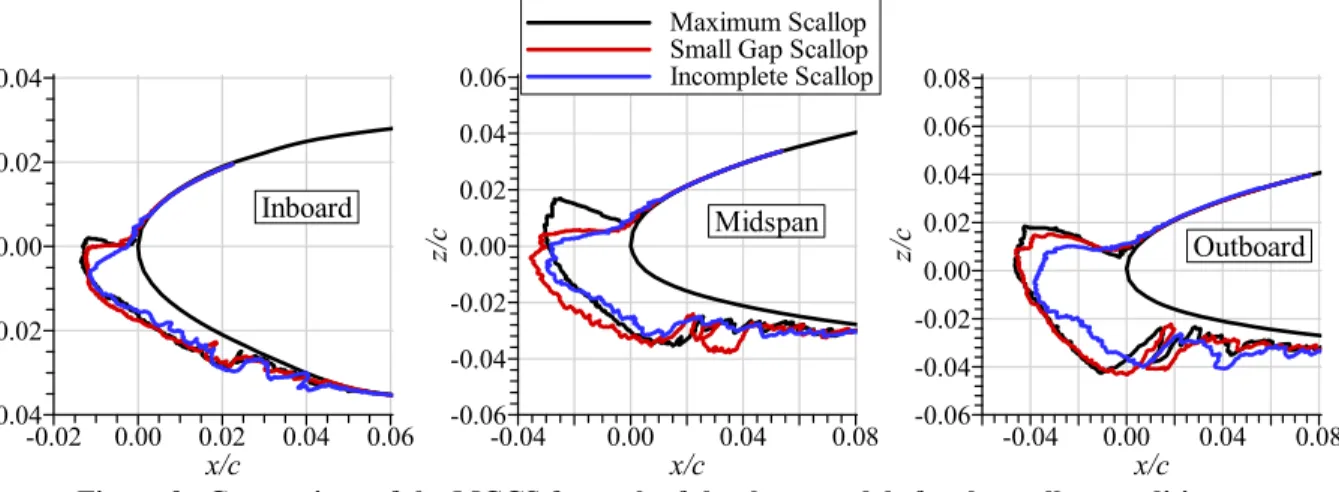
Further comparison of these ice geometries is presented in Figs. 9 and 10 that show the maximum combined cross section (MCCS) of each ice shape. The MCCS2 was derived from 30 section cuts over a six-inch spanwise segment of the 3D ice scan. The section cuts were projected onto a single plane and the maximum outer boundary was obtained. The resulting MCCS profile represents the outermost extent of the ice shape over that six-inch segment. Figure 9 compares the scallop ice formations accreted at different temperatures. The MCCS show some variation in the overall size, but the main differences between these cases are better illustrated in the photographs in Figs. 4, 5 and 6. Figure 10 shows the comparison for the Streamwise/Rime and WB33 configurations relative to the Maximum Scallop case for reference. Here there is a much larger variation in the cross section owning to the more significant differences in the icing conditions.
Figure 9. Comparison of the MCCS for each of the three models for the scallop conditions.
Figure 10. Comparison of the MCCS for each of the three models for the Streamwise/Rime and WB33 ice shapes relative to the Maximum Scallop case.
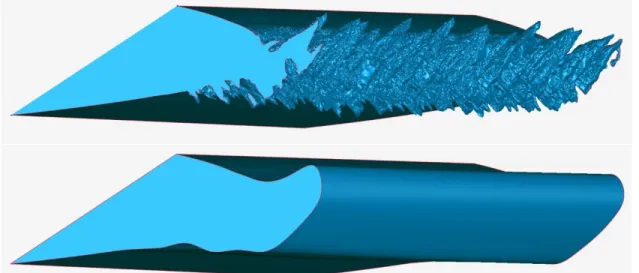
The various 3D ice geometries detailed in this section were used to create full-span artificial ice shapes for aerodynamic testing. Camello et al.,29 describe the process used to create the full-span, high-fidelity artificial ice shapes. In this case, “high-fidelity” means that the artificial ice shapes contained nearly all of the three-dimensional features depicted in Figs. 4-8. Camello et al.,29 also describe the methodology used to create lower-fidelity versions of these ice shapes. “3D smooth” ice shapes were also created from the high-fidelity geometry by taking MCCS-equivalent section cuts along the span, smoothing these cuts and then lofting them into a solid geometry. The 3D smooth ice shapes vary along the span of the wing, but do not contain any scallop type features, feathers or other ice roughness. A comparison of the high-fidelity and 3D-smooth geometries is shown in Fig. 11. In some cases, 46-grit silicon carbide grains were glued to the 3D smooth geometry to simulate ice roughness. FAA Advisory Circular 25-25A suggests a height of 3 mm on the full-scale reference geometry. This height is approximately equivalent to 46 grit size on the 13.3% scale model. The grit was applied with “full coverage” meaning that all of the surface was entirely covered with the silicon carbide grains. These lower-fidelity simulations were designed and built for the Maximum Scallop, Streamwise/Rime and WB33 ice shapes.
x/c z/ c -0.02 0.00 0.02 0.04 0.06 -0.04 -0.02 0.00 0.02 0.04 Inboard x/c z/ c -0.04 0.00 0.04 0.08 -0.06 -0.04 -0.02 0.00 0.02 0.04 0.06 Maximum Scallop Small Gap Scallop Incomplete Scallop Midspan x/c z/ c -0.04 0.00 0.04 0.08 -0.06 -0.04 -0.02 0.00 0.02 0.04 0.06 0.08 Outboard x/c z/ c -0.02 0.00 0.02 0.04 0.06 -0.04 -0.02 0.00 0.02 0.04 Inboard x/c z/ c -0.04 0.00 0.04 0.08 -0.06 -0.04 -0.02 0.00 0.02 0.04 0.06 Maximum Scallop Streamwise/Rime WB33 Midspan x/c z/ c -0.04 0.00 0.04 0.08 -0.06 -0.04 -0.02 0.00 0.02 0.04 0.06 0.08 Outboard
Figure 11. Comparison of high-fidelity artificial ice shape geometry (top) with the lower-fidelity, 3D smooth geometry (bottom).
F. Flow Visualization
Fluorescent mini-tuft flow visualization was employed during most of the angle of attack sweeps performed in this test campaign. The mini-tuft material was 0.006 in diameter fluorescent fishing line. The tufts were approximately 1.2 in long and were applied to the model upper surface using 0.002 in thick tape. The general layout of the tufts can be seen in Fig. 2 (right image). Continuous UV blacklight was used to illuminate the mini-tufts during the angle of attack sweeps. The tuft motion was recorded using two high-definition video cameras oriented at different viewing angles. The videos were annotated in real time with the model angle of attack. The tufts were applied to the wing for the tripped and iced-wing configurations. Comparison of force-balance data with and without the tufts located downstream of the upper-surface boundary-layer trip showed little to no effect of the tufts on the lift, drag and pitching moment.
IV. Results and Discussion
The primary aim of this paper is to report on the effects of Reynolds and Mach number on the clean- and iced-wing aerodynamic performance. A significant portion of this analysis was assigned to defining appropriate performance parameters such as maximum lift, stall angle and the like. Such parameters allow for analysis of trends in the data. Therefore, this section contains definition and discussion of these parameters. As an important primer, a brief initial look at the iced-wing aerodynamic performance is presented.
A. Effect of 3D, High-Fidelity, Artificial Ice Shapes on Wing Performance
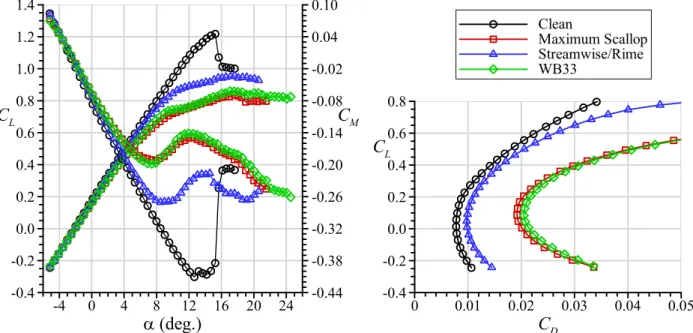
As described in Section II.D, there were five different 3D, high-fidelity artificial ice shape configurations created for this test campaign. The aerodynamic performance effect of these ice shapes on the CRM65 wing is summarized in Figs. 12 and 13 at the highest Reynolds number of 11.9×10⁶ with M = 0.23. In Fig. 12, the main variation in artificial ice-shape geometry was the level of three-dimensionality associated with the degree of scallop formation. The Maximum Scallop configuration, with the most clearly defined scallop formations, resulted in the highest drag and lowest maximum lift. The drag was clearly lower and maximum lift was clearly higher for the Small Gap and Incomplete Scallop configurations where the scallop features were less well defined and generally smaller. These results show the effect of variation scallop features on the wing aerodynamic performance. Figure 13 shows the effect on aerodynamic performance from the two remaining high-fidelity artificial ice-shape configurations. The Maximum Scallop configuration is also plotted as a point of reference back to Fig. 12. These results show that the adverse aerodynamic effect of a streamwise or rime ice configuration was significantly less than the other configurations consistent with its smaller overall thickness and 3D variation. In contrast, the WB33 configuration resulted in deleterious aerodynamic effects that were very similar to the Maximum Scallop configuration. This is significant because the WB33 configuration was based upon App. C airplane certification conditions whereas the Maximum Scallop configuration was not.
The lift curves shown in Figs. 12 and 13 for the wing with artificial ice shapes were characterized by some common features relative to the clean wing configuration. These lift curve characteristics were related to changes in
the pitching moment that is also plotted against angle of attack for direct comparison. For the iced-wing configuration, the lift curve slope begins to decrease significantly in the same angle of attack range where the pitching moment reaches the first local minimum. For example, consider the Maximum Scallop configuration for angles of attack between 6 and 8 deg where CM approaches a local minimum and the lift curve indicates a significant
departure from the clean configuration. The data show that CL continues to increase for the iced-wing
configurations up to relatively high angles of attack. These characteristics associated with the iced-wing lift curves in the stall regions prompted analysis designed to clearly identify a set of performance metrics used to summarize the large data set from this test campaign. This analysis is described in the next section.
Figure 12. Comparison of iced-wing performance effects for Maximum Scallop, Small Gap Scallop and Incomplete Scallop, 3D, high-fidelity, artificial ice shapes at Re = 11.9×10⁶ and M = 0.23.
Figure 13. Comparison of iced-wing performance effects for Maximum Scallop, Streamwise/Rime and WB33, 3D, high-fidelity, artificial ice shapes at Re = 11.9×10⁶ and M = 0.23.
C
D 0 0.01 0.02 0.03 0.04 0.05 -0.4 -0.2 0.0 0.2 0.4 0.6 0.8 Clean Maximum Scallop Small Gap Scallop Incomplete ScallopC
L
(deg.)
-4 0 4 8 12 16 20 24 -0.4 -0.2 0.0 0.2 0.4 0.6 0.8 1.0 1.2 1.4 -0.44 -0.38 -0.32 -0.26 -0.20 -0.14 -0.08 -0.02 0.04 0.10C
MC
LC
D 0 0.01 0.02 0.03 0.04 0.05 -0.4 -0.2 0.0 0.2 0.4 0.6 0.8 Clean Maximum Scallop Streamwise/Rime WB33C
L
(deg.)
-4 0 4 8 12 16 20 24 -0.4 -0.2 0.0 0.2 0.4 0.6 0.8 1.0 1.2 1.4 -0.44 -0.38 -0.32 -0.26 -0.20 -0.14 -0.08 -0.02 0.04 0.10C
MC
LB. Definition of Aerodynamic Performance Parameters 1. Lift-based Parameters
Iced aerodynamics has traditionally focused on maximum lift coefficient and the corresponding angle of attack as the most significant and easily identifiable performance parameters. Maximum lift coefficient is defined as the first local maximum in the lift curve with the corresponding angle of attack designated as the stall angle. Using the clean configuration as an example, CL,max =1.22 at αstall = 15.2 deg (cf. Fig. 12). For the iced-wing configurations
shown in Figs. 12 and 13, the maximum lift coefficients are fairly well defined by a local maximum. However, these CL,max values are associated with stall angles that are larger than for the clean wing. The iced-wing
configurations shown in Fig. 12 have stall angles ranging from 15.6 to 19.6 deg. In many other cases, the corresponding stall angles were also higher than the clean-wing value, as high as αstall = 22.7 deg. This represents a
fundamental difference from past research on straight wings or airfoils with large, leading-edge artificial ice shapes where the stall angle was lower the clean value. The lift curves for some configurations acquired at different Reynolds and Mach number conditions exhibited poorly defined local maxima where there was more of a “plateau” in the lift curve instead of a well-defined “peak.” Therefore the use of maximum lift coefficient and stalling angle may not necessarily be indicative of the stall progression on the swept, CRM65 wing with artificial ice shapes. The large reduction of lift-curve slope shown for the iced-wing configurations in Figs. 12 and 13 indicates significant flow separation. This separation occurs on the outboard portions of the wing that is represented in Figs. 12 and 13 by the changes in the pitching-moment curve. The outboard flow separation has also been determined through analysis of the flow visualization and surface-pressure distributions to be presented later in this section. These observations led to the identification of an additional performance metric that was associated with the change in the pitching-moment coefficient.
In 1957, Furlong and McHugh published a National Advisory Committee for Aeronautics (NACA) technical report summarizing the low-speed aerodynamic characteristics of swept wings based upon all known data collected through August 15, 1951.30 Furlong and McHugh identified a performance-based parameter called “usable” lift or “inflection” lift based upon their review of previous work. For convenience, the authors assumed that the quarter-chord MAC location was coincident with the airplane center of gravity. Therefore, the longitudinal stability could be referred to as either stable or unstable depending upon the slope of the pitching-moment curve with respect to angle of attack. The change from a negative slope to a positive slope thus indicated a change from a longitudinally stable to unstable situation. The term inflection lift refers to the local minimum in the CM vs α curve representing the
change in slope. The authors also clarified that the term usable lift coefficient represents the lift coefficient beyond which stall control is required. This interpretation of usable lift implies that a certain amount of flow separation on the wing has crossed some threshold such that this value of the usable lift coefficient may be more significant than the absolute value of the maximum lift coefficient. This interpretation of usable lift is applicable to the iced-wing aerodynamic effects observed within the present data set.
The 3D, high-fidelity Maximum Scallop configuration can be used as an example to further illustrate the usable lift coefficient as a meaningful performance metric. As shown in Fig. 12, the first local minimum in CM (CM,min =
-0.19) occurred at αuse = 7.9 deg and CL,use = 0.77. The corresponding distribution of wing upper-surface pressure is
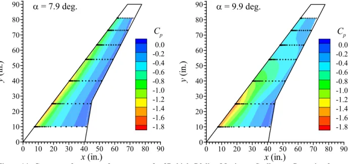
shown in Fig. 14. These contours were based upon a linear interpolation of the discrete pressure-tap data. The pressure taps used for the interpolation are shown on these plots as small open circles. Owing to this interpolation, any local flow effects that might have occurred between the pressure taps rows will not be revealed in these contours. Instead, the contours provide an overall look at the upper-surface pressure distribution. With this description in mind, the pressure contours for α = 7.9 deg in Fig. 14 show that the flow over the wing was well behaved with fairly uniform streamwise and spanwise variations in surface pressure. This picture is contrasted with the contour for α = 9.9 deg. where there was a large redistribution of pressure. The chordwise and spanwise uniformity no longer existed at this angle of attack. The pressure contours indicate likely flow separation outboard of pressure row 4 (y = 54.0 in; y/b = 0.6). While the coefficient of lift continued to increase with angle of attack up to 17.6 deg, the regions of separated flow also continued to increase in size. Thus, the identified usable lift coefficient (CL,use = 0.77 at αuse = 7.9 deg) provides an indication of the lift coefficient that can be attained in this
configuration before significant flow separation develops over the wing.
This example illustrates how the concept of usable lift can be employed to describe where the wing begins to stall in a way that is consistent with the original definition proposed by Furlong and McHugh.30 It is important to note that the inflection point, or first local minimum, in the pitching moment that defines CL,use is not always well
defined. As an example, consider the Small Gap Scallop configuration in Fig. 12. The CM curve tends to flatten out
in the region of the first local minimum at α = 7.4 deg which is follow by a second minimum at α = 9.9 deg. For this configuration there was not as significant of a change in the stall progression over these angles of attack as
illustrated in the previous paragraph for the Maximum Scallop configuration. This type of ambiguity in the usable lift coefficient is analogous to the situation in defining the maximum lift coefficient where the lift curve tends to reach a plateau rather than having a well-defined local maximum. Therefore, the information provided by both CL,use
and CL,max can be taken together as complementary performance-based parameters.
Figure 14. Contours of upper-surface pressure for 3D, high-fidelity, Maximum Scallop configuration for α = 7.9 and 9.9 deg at Re = 11.9×10⁶ and M = 0.23.
2. Drag-based Parameters
The artificial ice-shape configurations developed for aerodynamic testing were partly based upon typical airplane holding scenarios in App. C conditions. As a result, the leading-edge ice shapes were large as shown in Section II.D. In 2001, Lynch and Khodadoust published, “a systematic and comprehensive review, correlation, and assessment of test results available in the public domain which address the aerodynamic performance and control degradations caused by various types of ice accretions on the lifting surfaces of fixed wing aircraft.”31 The authors directly address the importance of drag penalties due to leading-edge ice accretion stating that such penalties are a concern because they can lead to reductions in aircraft climb and acceleration gradients, range and speed. They point out that accidents and incidents have been reported with autopilots not augmented with autothrottle during icing exposure where the airspeed can be reduced to stall entry without warning. In addition to these practical considerations, it is important from a research perspective to understand how the drag coefficient may be affected by changes in Reynolds number and Mach number.
Lynch and Khodadoust31 suggested two conditions for the assessment of icing-related drag penalties. The first condition is simply the value of the minimum drag coefficient. For the clean and iced-wing configurations in this paper, the minimum drag coefficient is always near zero lift because of the influence of induced drag for non-zero lift coefficients. The other condition that Lynch and Khodadoust recommend is that corresponding to a flight speed 30% above the 1-g stall speed (Vs,1g) for the clean reference geometry. This equivalent to a lift coefficient that is
59% of CL,max for the clean wing. As discussed later in Section III.C, there is a significant dependence of the clean
wing CL,max upon Reynolds and Mach number, with values ranging from 0.98 to 1.23. In order to simplify the
analysis of iced-wing drag penalties, a reference value of CL = 0.6 was selected which corresponds to a CL,max =
1.014 for a speed of 1.3Vs,1g. The reference value of CL = 0.6 was also selected because it is lower than all of the
values of CL,use identified for these iced-wing configurations. This means that the drag penalties associated with this
lift coefficient are still within the range of lift coefficient prior to the onset of significant stall progression on the wing. All of the drag-polar data were analyzed to determine the minimum drag coefficient and the drag coefficient at CL = 0.6.
C. Clean Wing Reynolds and Mach Number Results
The pressurization capability of the F1 wind tunnel was fully exploited to investigate the independent effects of Reynolds and Mach number on the 13.3% scale wing aerodynamics. As shown in Table 1, the effect of Reynolds
x
(in.)
y
(i
n.
)
0 10 20 30 40 50 60 70 80 90 0 10 20 30 40 50 60 70 80 90 0.0 -0.2 -0.4 -0.6 -0.8 -1.0 -1.2 -1.4 -1.6 -1.8C
p
= 7.9 deg.
x
(in.)
y
(i
n.
)
0 10 20 30 40 50 60 70 80 90 0 10 20 30 40 50 60 70 80 90 0.0 -0.2 -0.4 -0.6 -0.8 -1.0 -1.2 -1.4 -1.6 -1.8C
p
= 9.9 deg.
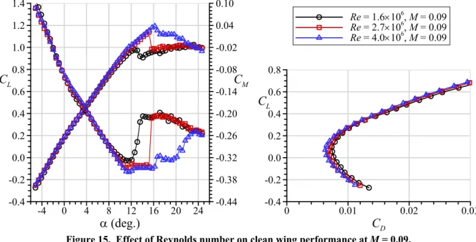
number was measured at constant Mach numbers of 0.09, 0.18, 0.23 and 0.27. Figure 15 shows a comparison of lift, drag and pitching moment for the M = 0.09 conditions. Readily observable is the significant increase in CL,max and
αstall over this range of Reynolds number. Maximum lift coefficient increased approximately 20% from 0.98 to 1.19
while stall angle increased 3.6 deg from 12.6 deg to 16.2 deg. as the Reynolds number was increased from 1.6×10⁶ to 4.0×10⁶. The data illustrate the behavior of C
L,use as identified by the minimum CM. For Re = 1.6×10⁶, the value
of CL,use was 0.95 which was very close to the value of CL,max = 0.98. As Reynolds number was increased the
minimum CM occurred at approximately the same angle of attack while the lift coefficient continued to increase to
stall. There was, however, a noticeable reduction in the lift-curve slope that approximately corresponded to CM,min.
The drag polar plotted in Fig. 15 indicates a reduction in the minimum drag coefficient of 11 drag counts (ΔCD,min =
0.0011) over this range of Reynolds number. There was also a reduction in drag coefficient at CL = 0.6 of 13 drag
counts (ΔCD,0.6 = 0.0013).
Figure 15. Effect of Reynolds number on clean wing performance at M = 0.09.
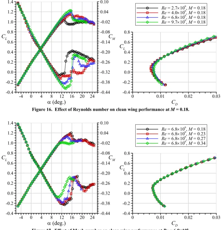
Similar significant changes in the wing performance characteristics were also observed as the Reynolds number was increased to 9.7×10⁶ at M = 0.18 as illustrated in Fig. 16. Maximum lift coefficient was again increased by approximately 20% from 1.04 at Re = 2.7×10⁶ to 1.23 at Re = 9.7×10⁶ with a corresponding increase in stall angle from 13.1 deg to 15.2 deg. The minimum in CM was coincident with a distinct reduction in the lift-curve slope while
CL continued to increase toward stall. There was a reversal in the trend with respect to the minimum drag
coefficient. For these data, the lowest value of CD,min was measured at Re = 4.0×10⁶ with CD,min increasing at the two
higher Reynolds numbers. At CL = 0.6, the drag coefficient was lowest for Re = 9.6×10⁶ with a value of 0.0228 and
increased to 0.0250 at Re = 2.7×10⁶. Reynolds number was further increased to Re = 11.9×10⁶ at M = 0.23. Data on the clean wing for this condition were presented in Figs. 12 and 13 and the Reynolds number trends at M = 0.23 were similar to those shown in Fig. 16.
As shown in Table 1, the effect of Mach number was measured at constant Reynolds numbers of 2.7×10⁶, 4.0×10⁶, and 6.8×10⁶. Figure 17 shows a comparison of lift, drag and pitching moment for the Re = 6.8×10⁶ conditions. The largest effect of Mach number was observed in the maximum lift coefficient and stall angle. Maximum lift coefficient decreased approximately 20% from 1.20 to 1.01 while the stalling angle decreased 3.6 deg from 15.7 deg to 12.1 deg. as the Mach number was increased from 0.18 to 0.34. There was a change in the stalling characteristics at M = 0.34, where the lift coefficient did not decrease significantly as the angle of attack was increased past CL,max. Also for the M = 0.34 condition, the value of CL,use = 0.97 was close to CL,max while there was
a much larger difference between these values for the lower Mach numbers. As indicated in Fig. 17, there was very little measureable change in the drag coefficient or pitching-moment coefficient outside of the stall region. Very similar trends were observed for the Mach number variation at a constant Reynolds number of 2.7×10⁶ and 4.0×10⁶.
C
D 0 0.01 0.02 0.03 -0.4 -0.2 0.0 0.2 0.4 0.6 0.8 Re= 1.6106,M= 0.09 Re= 2.7106,M= 0.09 Re= 4.0106,M= 0.09C
L
(deg.)
-4 0 4 8 12 16 20 24 -0.4 -0.2 0.0 0.2 0.4 0.6 0.8 1.0 1.2 1.4 -0.44 -0.38 -0.32 -0.26 -0.20 -0.14 -0.08 -0.02 0.04 0.10C
MC
LFigure 16. Effect of Reynolds number on clean wing performance at M = 0.18.
Figure 17. Effect of Mach number on clean wing performance at Re = 6.8×10⁶.
The maximum lift coefficient and usable lift coefficients were extracted from the performance data and are plotted as a function of Reynolds number in Fig. 18. Clearly shown is the trend of increasing CL,max and CL,use with
increasing Reynolds number. These variation were non-linear with most of the increases in CL,max and CL,use
occurring for Reynolds number less than 6.0×10⁶. These curves do suggest, however, that the maximum lift coefficient for the clean wing may still continue to increase for Reynolds numbers greater than 12.0×10⁶. The variation in CL,max with Reynolds number is generally consistent with a significant amount of airfoil section data
compiled by Broeren et al.16 where the largest increases were observed for Re less than 6.0×10⁶. Data were reported for NACA 23012, NACA 0012, GLC-305 and NLF-0414 airfoils for Reynolds numbers up to 16.0×10⁶ and M = 0.20. Experimental data for swept wings are more challenging to compare because of the inherent dependence upon the wing configuration such as sweep angle, aspect ratio, twist, taper and other parameters. Koven and Graham32 documented the performance of an aspect ratio 6 wing having 37 deg leading edge sweep angle that was comparable
C
D 0 0.01 0.02 0.03 -0.4 -0.2 0.0 0.2 0.4 0.6 0.8 Re= 2.7106,M= 0.18 Re= 4.0106,M= 0.18 Re= 6.8106,M= 0.18 Re= 9.7106,M= 0.18C
L
(deg.)
-4 0 4 8 12 16 20 24 -0.4 -0.2 0.0 0.2 0.4 0.6 0.8 1.0 1.2 1.4 -0.44 -0.38 -0.32 -0.26 -0.20 -0.14 -0.08 -0.02 0.04 0.10C
MC
LC
D 0 0.01 0.02 0.03 -0.4 -0.2 0.0 0.2 0.4 0.6 0.8 Re= 6.8106,M= 0.18 Re= 6.8106,M= 0.23 Re= 6.8106,M= 0.27 Re= 6.8106,M= 0.34C
L
(deg.)
-4 0 4 8 12 16 20 24 -0.4 -0.2 0.0 0.2 0.4 0.6 0.8 1.0 1.2 1.4 -0.44 -0.38 -0.32 -0.26 -0.20 -0.14 -0.08 -0.02 0.04 0.10C
MC
Lto the 13.3% scale CRM65 wing in the present study. Tests were conducted at the Langley 19-foot pressure tunnel where the Reynolds number was varied from 2.0×10⁶ to 9.4×10⁶ with corresponding Mach number variation from 0.08 to 0.18. Consistent with the present data, CL,max increased from approximately 0.98 at Re = 2.0×10⁶ and M =
0.08 to 1.27 at Re = 6.8×10⁶ and M = 0.13 with no further increase as Re and M increased.
The data in Fig. 18 also show that Mach number had the opposite effect, where CL,max and CL,use decreased with
increasing Mach Number. This effect is summarized better in Fig. 19 for each of the Reynolds number conditions. The data indicate that the maximum lift coefficient could decrease with further increases in Mach number greater than 0.34. However, usable lift coefficient approached a near-constant value for M > 0.27. The trend observed in
CL,max was again consistent with the large volume of airfoil data presented in Broeren et al.16 with the decreasing
values persisting for M > 0.34. As noted in the previous paragraph, finding comparable swept-wing data is challenging. In one report, Edwards and Boltz33 documented the aerodynamics of an aspect ratio 6 wing having 37.25 deg leading edge sweep angle for Mach number variations from 0.18 to 0.94 at a constant Reynolds number of 2.0×10⁶. This wing exhibited a decrease in C
L,max from approximately 1.01 to 0.90 as Mach number was increased
from 0.18 to 0.40. Unfortunately, the authors did not report CL,max values for larger Mach numbers, nor did they
provide any explanation.
Figure 18. Effect of Reynolds number on maximum and usable lift coefficients for the clean wing for various Mach numbers.
The variation in drag performance with changes in Reynolds and Mach number is summarized in Fig. 20 for the clean wing. These plots show immediately that there was no effect of Mach number on CD,min and CD,0.6 over the
range tested. These results were consistent with the data reported by Edwards and Boltz33 described in the previous paragraph. In terms of Reynolds number dependence, opposite trends were observed for CD,min and CD,0.6. The
former coefficient exhibited a minimum at Re = 4.0×10⁶ as noted earlier in this section with increasing values measured for increasing Reynolds number. In contrast, CD,0.6 was a maximum at the lowest Re and decreased with
increasing Re.
The performance-based parameter trends shown in Figs. 18-20 exhibited classic Reynolds and Mach number dependence based upon known comparisons to comparable data in the archival literature. This evaluation of the clean-wing performance thus provides further confidence in the present data set over this range of Re and M. It should be noted for completeness, however, that the typical Reynolds numbers for a CRM65 size airplane are significantly higher. As discussed in Section II.D, the icing scenarios were based upon holding operations. Wiberg et al.34 provide a summary of the corresponding Reynolds and Mach numbers that range from 24.8×10⁶ to 32.9×10⁶ and 0.35 to 0.46, respectively. Therefore, the maximum Reynolds number for the present data was at least a factor of two lower than the fight reference conditions. At the maximum Mach number of 0.34, the Reynolds number was nearly a factor of four lower than the flight reference conditions. However, the maximum Mach number of 0.34 was significantly closer to the flight reference conditions. The largest impact of these differences would be estimating
Reynolds Number (106) 1 2 3 4 5 6 7 8 9 10 11 12 0.5 0.6 0.7 0.8 0.9 1.0 1.1 1.2 1.3
C
L,max Reynolds Number (106) 1 2 3 4 5 6 7 8 9 10 11 12 0.5 0.6 0.7 0.8 0.9 1.0 1.1 1.2 1.3 M= 0.09 M= 0.18 M= 0.23 M= 0.27C
L,useCL,max for the clean-wing configuration. Since both Reynolds and Mach number effects are significant (cf. Fig. 19) it
is difficult to extrapolate the clean-wing CL,max beyond the acquired data range.
Figure 19. Effect of Mach number on maximum and usable lift coefficients for the clean wing for various Reynolds numbers.
Figure 20. Effect of Reynolds number on minimum and CL = 0.6 drag coefficients for the clean wing various
Mach numbers.
Another implication for the effects of Reynolds and Mach number on the performance of the clean wing is the planned comparison between the present data and results from aerodynamic testing conducted at the WSU wind tunnel. Reynolds and Mach number cannot be matched between the two wind tunnels because the WSU facility is not pressurized and the CRM65 model was smaller than the F1 wind-tunnel model. WSU wind tunnel data were acquired at Re = 0.8×10⁶, 1.6×10⁶, and 2.4×10⁶ with corresponding M = 0.09, 0.18 and 0.27, respectively. Therefore, there was some overlap in the conditions. The data presented in this section show that both Reynolds and Mach number must be respected when comparing the clean wing aerodynamic data from the respective facilities. The companion paper by Lee5 presents these comparisons.
Mach Number 0.05 0.10 0.15 0.20 0.25 0.30 0.35 0.5 0.6 0.7 0.8 0.9 1.0 1.1 1.2 1.3
C
L,max Mach Number 0.05 0.10 0.15 0.20 0.25 0.30 0.35 0.5 0.6 0.7 0.8 0.9 1.0 1.1 1.2 1.3 Re= 2.7106 Re= 4.0106 Re= 6.7 to 6.8106C
L,use Reynolds Number (106) 1 2 3 4 5 6 7 8 9 10 11 12 0.000 0.005 0.010 0.015 0.020 0.025 0.030C
D,min Reynolds Number (106) 1 2 3 4 5 6 7 8 9 10 11 12 0.000 0.005 0.010 0.015 0.020 0.025 0.030 M= 0.09 M= 0.18 M= 0.23 M= 0.27 M= 0.34C
D,0.6D. Effect of Boundary-Layer Trips and Mini-Tufts
A series of tests were conducted with boundary-layer trips applied to the model as detailed in Section II.C. After these tests were completed the fluorescent mini-tufts were added to the model as detailed in Section II.F. It was assumed that if there was no measurable effect of the tufts on the wing with boundary-layer trips, then there would be no measurable effect of the tufts on the wing with artificial ice shapes. For all of the runs with trips and with trips plus tufts there was no significant change in lift coefficient relative to the clean wing which was expected since the trips and tufts were placed downstream of the leading-edge hilite. For example, the Reynolds and Mach number trends for CL,max were identical to those shown in Figs. 18 and 19. The largest changes were observed in the
minimum drag coefficient which are illustrated in Fig. 21. Since Mach number was observed to have little to no effect on drag coefficient, data from all Mach numbers were combined into a single series in Fig. 21. This affords a clearer comparison of the Reynolds number effects. The data show that the trips increased CD,min for all but the
highest Reynolds number of 11.9×10⁶. This was expected since the trips heights were based upon the lowest Reynolds number and it was expected that natural boundary-layer transition would move forward to the leading-edge region for higher Reynolds numbers. The trips increased the drag coefficient at CL = 0.6 up to a Reynolds
number of about 4.0×10⁶. Only a subset of the Reynolds and Mach number matrix was performed for the wing with mini-tuft applied to the upper surface. Thus, the data points in Fig. 21 were not connected with line segments as for the other data. These data show that an additional drag increment due to the tufts was measured for Re = 1.6×10⁶. However, this additional drag was small relative to the much larger increases observed for the iced-wing configurations. Therefore, the data show that the presence of the mini-tufts did not have a measurable effect on the iced-wing aerodynamics.
Figure 21. Effect of boundary-layer trips and mini-tufts on minimum and CL = 0.6 drag coefficients for
various Reynolds and Mach numbers. E. Iced Wing Reynolds and Mach Number Results
The pressurization capability of the F1 wind tunnel was fully exploited to investigate the independent effects of Reynolds and Mach number on the 13.3% scale wing aerodynamics with the various combinations of high- and low-fidelity artificial ice shapes attached to the wing leading edge. Exemplary results for the effect of Reynolds number at a constant Mach number of 0.18 are plotted in Fig. 22 for the wing with the 3D, high-fidelity, Maximum Scallop artificial ice shape. These data show that there was virtually no change in CL and CM vs angle of attack as Reynolds
number was increased from 2.7×10⁶ to 9.5×10⁶. The largest changes in performance were observed in drag coefficient. For example, CD,min decreased by 12 drag counts (ΔCD,min = 0.0012) as Reynolds number was increased
from 2.7×10⁶ to 9.5×10⁶. Figure 23 provides results from the same configuration as Mach number was increased from 0.09 to 0.27 at constant Re = 4.0×10⁶. There was a measurable effect of Mach number on the iced wing stall as
CL,max and αstall decreased from 0.87 and 18.1 deg to 0.83 and 16.5 deg, respectively as the Mach number was
increased from 0.09 to 0.18. For Mach numbers greater than 0.18, there was very little or no variation in CL,max and
Reynolds Number (106) 1 2 3 4 5 6 7 8 9 10 11 12 0.000 0.005 0.010 0.015 0.020 0.025 0.030
C
D,min Reynolds Number (106) 1 2 3 4 5 6 7 8 9 10 11 12 0.000 0.005 0.010 0.015 0.020 0.025 0.030 Clean,M= 0.09 to 0.34 Trips,M= 0.09 to 0.34 Trips + Tufts,M= 0.09 to 0.34C
D,0.6αstall. Changes in Mach number from 0.09 to 0.34 had little to no effect on drag coefficient, which is consistent with
the data presented previously for the clean wing and wing with boundary-layer trips and mini tufts.
Figure 22. Effect of Reynolds number on iced-wing performance for 3D, high-fidelity, Maximum Scallop artificial ice shape at M = 0.18.
Figure 23. Effect of Mach number on iced-wing performance for 3D, high-fidelity, Maximum Scallop artificial ice shape at Re = 4.0×10⁶.
The effect of Reynolds and Mach number variation on the iced-wing lift coefficient is summarized in Fig. 24 for the 3D, high-fidelity Maximum Scallop configuration. There was an effect of Mach number between 0.09 and 0.18 where CL,max decreased from 0.87 to 0.83 at Re = 4.0×10⁶ as noted in the previous paragraph. However, the data
show that CL,max was virtually independent of Reynolds number over the range tested. These observations regarding
the effects of Reynolds and Mach number are consistent with the large volume of iced airfoil data acquired over many years for various airfoils and artificial ice shapes.14,16 An analogous observation can also be made for C
L,use
where there was an effect of Mach number at Re = 6.8×10⁶, with the value decreasing from 0.65 to 0.63 as Mach number was increased from 0.23 to 0.27. There was no further decrease in CL,use as Mach number was increased to