Drofelnik, Jernej (2017)
Massively parallel time- and frequency-domain
Navier-Stokes Computational Fluid Dynamics analysis of wind turbine and
oscillating wing unsteady flows.
PhD thesis.
http://theses.gla.ac.uk/8284/
Copyright and moral rights for this work are retained by the author
A copy can be downloaded for personal non-commercial research or study, without prior permission or charge
This work cannot be reproduced or quoted extensively from without first obtaining permission in writing from the author
The content must not be changed in any way or sold commercially in any format or medium without the formal permission of the author
When referring to this work, full bibliographic details including the author, title, awarding institution and date of the thesis must be given
Enlighten:Theses
http://theses.gla.ac.uk/
frequency–domain Navier–Stokes
Computational Fluid Dynamics
analysis of wind turbine and
oscillating wing unsteady flows
Jernej Drofelnik
Submitted in fulfilment of the requirements for the Degree of
Doctor of Philosophy
School of Engineering
College of Science and Engineering
University of Glasgow
Abstract
Increasing interest in renewable energy sources for electricity production complying with stricter environmental policies has greatly contributed to further optimisation of existing devices and the development of novel renewable energy generation systems. The research and development of these advanced systems is tightly bound to the use of reliable design methods, which enable accurate and efficient design. Reynolds–averaged Navier–Stokes Computational Fluid Dynamics is one of the design methods that may be used to accurately analyse complex flows past current and forthcoming renewable energy fluid machinery such as wind turbines and oscillating wings for marine power generation. The use of this simulation technology offers a deeper insight into the com-plex flow physics of renewable energy machines than the lower–fidelity methods widely used in industry. The complex flows past these devices, which are characterised by highly unsteady and, often, predominantly periodic behaviour, can significantly affect power production and structural loads. Therefore, such flows need to be accurately predicted.
The research work presented in this thesis deals with the development of a novel, accurate, scalable, massively parallel CFD research code COSA for general fluid–based renewable energy applications. The research work also demonstrates the capabilities of newly developed solvers of COSA by investigating complex three–dimensional unsteady periodic flows past oscillating wings and horizontal–axis wind turbines.
Oscillating wings for the extraction of energy from an oncoming water or air stream, feature highly unsteady hydrodynamics. The flow past oscillating wings may feature dynamic stall and leading edge vortex shedding, and is significantly three–dimensional due to finite–wing effects. Detailed understanding of these phenomena is essential for maximising the power generation efficiency. Most of the knowledge on oscillating wing hydrodynamics is based on two–dimensional low–Reynolds number computational fluid dynamics studies and experimental testing. However, real installations are expected to feature Reynolds numbers of the order of 1 million and strong finite–wing–induced losses. This research investigates the impact of finite wing effects on the hydrody-namics of a realistic aspect ratio 10 oscillating wing device in a stream with Reynolds number of 1.5 million, for two high–energy extraction operating regimes. The bene-fits of using endplates in order to reduce finite–wing–induced losses are also analyzed. Three–dimensional time–accurate Reynolds–averaged Navier–Stokes simulations using Menter’s shear stress transport turbulence model and a 30–million–cell grid are per-formed. Detailed comparative hydrodynamic analyses of the finite and infinite wings highlight that the power generation efficiency of the finite wing with sharp tips for the considered high energy–extraction regimes decreases by up to 20 %, whereas the maximum power drop is 15 % at most when using the endplates.
Horizontal–axis wind turbines may experience strong unsteady periodic flow regimes, such as those associated with the yawed wind condition. Reynolds–averaged Navier– Stokes CFD has been demonstrated to predict horizontal–axis wind turbine unsteady flows with accuracy suitable for reliable turbine design. The major drawback of con-ventional Reynolds–averaged Navier–Stokes CFD is its high computational cost. A time–step–independent time–domain simulation of horizontal–axis wind turbine peri-odic flows requires long runtimes, as several rotor revolutions have to be simulated before the periodic state is achieved. Runtimes can be significantly reduced by using
ing technology can be efficiently used for the analyses of complex three–dimensional horizontal–axis wind turbine periodic flows, and has a vast potential for rapid wind turbine design. The three–dimensional simulations of the periodic flow past the blade of the NREL 5–MW baseline horizontal–axis wind turbine in yawed wind have been selected for the demonstration of the effectiveness of the developed technology. The comparative assessment is based on thorough parametric time–domain and harmonic balance analyses. Presented results highlight that horizontal–axis wind turbine peri-odic flows can be computed by the harmonic balance solver about fifty times more rapidly than by the conventional time–domain analysis, with accuracy comparable to that of the time–domain solver.
Keywords: Compressible multigrid Navier–Stokes solvers, Computational fluid dynamics, Dynamic stall, Energy–extracting oscillating wing, Finite wing effects, Harmonic balance Navier–Stokes equations, Horizontal–axis wind turbine periodic aerodynamics, Fully coupled multigrid integration, Leading edge vortex shedding, Point–implicit Runge–Kutta smoother, Shear stress transport turbulence model
Contents
List of Figures X
List of Tables XI
Acknowledgements XII
Author’s Declaration XIII
Nomenclature XVII
1 Introduction 1
1.1 Renewable energy . . . 1
1.2 Computational fluid dynamics for oscillating wing devices . . . 2
1.3 Computational fluid dynamics for horizontal–axis wind turbines . . . . 7
1.3.1 NREL Phase VI wind turbine . . . 8
1.3.2 NREL 5–MW baseline wind turbine . . . 10
1.4 Harmonic balance method in computational fluid dynamics . . . 11
1.5 Motivation, aims and objectives . . . 12
1.6 Thesis outline . . . 15 2 Governing equations 17 2.1 Conservation laws . . . 17 2.2 Turbulence closure . . . 20 2.2.1 Reynolds–Favre averaging . . . 21 2.2.2 Boussinesq approximation . . . 21 2.2.3 k−ω SST turbulence closure . . . 21
2.3 Time–domain RANS and SST . . . 23
2.4 Arbitrary Lagrangian–Eulerian formulation of URANS and SST equa-tions in inertial frame . . . 25
2.5 Arbitrary Lagrangian–Eulerian formulation of URANS and SST equa-tions in non–inertial frame . . . 27
2.6 Harmonic balance formulation of Navier–Stokes Equations . . . 29
2.7 Boundary conditions . . . 34
2.7.1 Farfield . . . 34
2.7.2 Solid wall . . . 36
3.1.1 Convective fluxes . . . 38
3.1.2 Diffusive fluxes . . . 42
3.2 Calculation of cell face velocities . . . 45
3.3 Cut boundary condition . . . 47
3.4 Steady and multi–frequency periodicity boundary condition . . . 49
3.5 Fully coupled integration of steady equations . . . 51
3.6 Fully coupled integration of time–domain equations . . . 53
3.7 Fully coupled integration of harmonic balance equations . . . 55
4 Code parallelization 57 4.1 High Performance Computing . . . 57
4.2 Parallel computing with Message Passing Interface . . . 60
4.3 Data decomposition . . . 62
4.4 Message Passing Interface communications . . . 64
4.5 Parallel input/output . . . 66
4.6 Parallel scalability . . . 68
5 Validation 71 5.1 Summary of previously published validation cases . . . 72
5.2 Preliminary validation . . . 72
5.2.1 Delta wing . . . 72
5.2.2 ONERA M6 wing . . . 75
5.2.3 S809 airfoil . . . 80
5.3 H–Darrieus vertical–axis wind turbine . . . 83
5.4 Oscillating wing . . . 86
5.5 NREL Phase VI horizontal–axis wind turbine . . . 90
5.5.1 Physical and numerical set–up . . . 90
5.5.2 Aerodynamic analyses of 0◦ yaw case . . . 92
5.5.3 Aerodynamic analyses of 10◦ and 30◦ yaw cases . . . 101
6 Results 108 6.1 Oscillating wing devices . . . 108
6.1.1 Oscillating wing fundamentals . . . 108
6.1.2 Physical and numerical set–up . . . 111
6.1.3 Hydrodynamic analysis of case A . . . 118
6.1.4 Hydrodynamic analysis of case B . . . 127
6.1.5 Discussion . . . 135
6.2 Horizontal–axis wind turbines . . . 137
6.2.1 Aerodynamics of horizontal–axis wind turbines . . . 137
6.2.2 Horizontal–axis wind turbines in yawed wind condition . . . 140
6.2.3 Physical and numerical set–up . . . 142
6.2.4 Aerodynamic analyses . . . 146
6.2.5 Computational performance of the HB solver . . . 161
7 Conclusions 164 7.1 Summary and concluding remarks . . . 164
7.1.1 Oscillating wings . . . 164
7.1.2 Horizontal–axis wind turbines . . . 165 II
7.2 Future work . . . 166
Bibliography 179
A Numerical dissipation 180 B Convergence acceleration techniques 186
B.0.1 Local time stepping . . . 186 B.0.2 Implicit residual smoothing . . . 187 B.0.3 Multigrid . . . 188
C NREL Phase VI 193
1.1 Wingmill experimental setup. Taken from [1]. . . 3
1.2 Side view of the oscillating–wing hydropower generator. Taken from [2]. 3 1.3 Stingray Assembly. Taken from [3]. . . 4
1.4 The 100 kW Pulse tidal oscillating wing device. Taken from [4]. . . 4
1.5 An artistic impression of the 1.2 MW Pulse Tidal oscillating wing device. Taken from [5]. . . 5
1.6 Side and rear views of the experimental setup. Taken from [6]. . . 5
2.1 Finite control volume. . . 18
2.2 Cartesian rotating coordinate system. . . 28
3.1 One–sided extrapolation of flux interface. . . 39
3.2 Cartesian to generalised curvilinear coordinate transformation. . . 43
3.3 Sketch of a hexahedral cell. . . 46
3.4 Block, surrounded by the two rows of halo cells representing boundary conditions. . . 47
3.5 Representation of three different boundary patches on boundary face. . 48
3.6 Sectional slice of j–k plane through the interior domain and halo cells of patch 1. . . 48
3.7 Sketch of a sector, with two periodic boundaries. . . 49
3.8 Rotor with 3 blades at time t and ∆t. . . 51
4.1 Growth of supercomputing power. Taken from [7]. . . 58
4.2 Simple representation of block assignment to MPI processes of a 2D computational grid around cylindrical body. . . 63
4.3 Sketch of a common data file, where each MPI process reads a chunk of the data. . . 67
4.4 Parallel scalability analysis of algorithmic part of COSA HB MPI solver on ARCHER HPC system, using plunging wing test case. . . 69
4.5 Parallel scalability analysis of algorithmic part of COSA HB MPI solver on ARCHER HPC system, using HAWT test case. . . 70
5.1 Representation of computational domain of the delta wing test case. Only every second line in all three directions is plotted. . . 73
5.2 Slices of the vorticity magnitude at four chordwise positions, 30 %, 50 %, 70 % and 90 % of the root chord. The left semi–span represents the CFL3D solution, whereas the right semi–span represents the COSA so-lution. . . 74
5.3 Residual convergence histories of the CFL3D and COSA calculations. . 75
5.4 Experimental setup of the ONERA M6 wing. Taken from [8]. . . 75
5.5 Geometry of the ONERA M6 wing. Taken from [8]. . . 76
5.6 Representation of the computational domain and the wing surface grid of the ONERA M6 wing. Only every second line in all three directions is plotted. . . 77 5.7 Contours of the pressure coefficient cp along the wing span. Left plot:
The COSA result. Right plot: The NUMECA result. . . 78 5.8 Comparison of the pressure coefficient cp distributions along the chord
at seven spanwise positions for two CFD results and experimental results. 79 5.9 Grid for the S809 airfoil analysis. Left plot: complete domain. Right
plot: near–airfoil area. . . 80 5.10 The lift and drag coefficients vs. angle of attack of the S809 airfoil. . . 81 5.11 Pressure coefficientcp of the S809 airfoil for the three different values of
AoA. . . 82 5.12 H–Darrieus rotor sketch. . . 83 5.13 H–Darrieus rotor grid representation. Left: grid view in rotor region.
Right: grid view in airfoil region. . . 84 5.14 H–Darrieus rotor periodic profiles of torque coefficient of reference blade
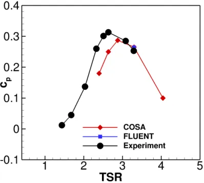
against azimuthal position θ computed with COSA and FLUENT sim-ulations. . . 84 5.15 H–Darrieus rotor Mach contours and streamlines in the reference blade
trailing edge region at azimuthal positionθ= 99o computed with COSA simulation (left) and FLUENT simulation (right). . . 85 5.16 Comparison of the nondimensionalized power curves of the H–Darrieus
rotor between COSA, FLUENT and experimental data. . . 86 5.17 Grid for the NACA0015 airfoil. . . 87 5.18 Comparison of the K and D–SA, K and D–SST and COSA solutions:
overall power coefficient (top), heaving power coefficient (middle), and pitching power coefficient (bottom). . . 88 5.19 Comparison of vorticity time sequences at t/T=0, 0.125, 0.25, for K
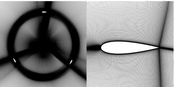
and D–SA, K and D–SST and COSA solutions (red: counter–clockwise vorticity, blue: clockwise vorticity). . . 89 5.20 NREL Phase VI sector grid representation. Top Left: Blade view, only
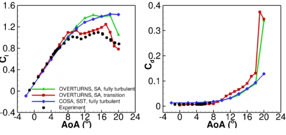
every fourth line in all directions is represented. Top right: near–airfoil area at 50 % of blade length. Bottom: complete domain. . . 91 5.21 Power curve of the NREL Phase VI turbine. For the experimental data,
sample minimum and maximum are also plotted. . . 93 5.22 Spanwise distribution of the normal force coefficients (left) and the
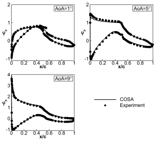
tan-gential force coefficients (right) for the six operating regimes of the NREL Phase VI blade: 7m/s, 10m/s, 13m/s, 15m/s, 20m/s and 25m/s. For the experimental data, sample minimum and maximum are also plotted. . . 94 5.23 Pressure coefficient cp distributions of the NREL Phase VI blade, for
the 7m/s case. . . 96 5.24 Pressure coefficient cp distributions of the NREL Phase VI blade, for
the 10m/s case. . . 97 5.25 Pressure coefficient cp distributions of the NREL Phase VI blade, for
the 13m/s case. . . 98 5.26 Pressure coefficient cp distributions of the NREL Phase VI blade, for
the 15m/s case. . . 98 5.27 Pressure coefficient cp distributions of the NREL Phase VI blade, for
the 20m/s case. . . 99
5.29 Skin friction lines on the suction side of the NREL Phase VI blade, computed with the COSA medium grid, for the six operating regimes: 7m/s, 10m/s, 13m/s, 15m/s, 20m/s and 25m/s. . . 100 5.30 Top view of the boom and instrumentation enclosure wake interference.
Taken from [9]. . . 101 5.31 Front view of the Phase VI HAWT. Shaded area is significantly affected
by the boom and instrumentation enclosure wake. Taken from [9]. . . . 102 5.32 Spanwise distribution of the normal force coefficients (left) and the
tan-gential force coefficients (right) at 7m/s and the yaw angle δ = 10◦, for the three azimuthal positions of the NREL Phase VI blade: θ = 210◦,
θ = 270◦, and θ = 330◦. For the experimental data, sample minimum and maximum are also plotted. . . 103 5.33 Spanwise distribution of the normal force coefficients (left) and the
tan-gential force coefficients (right) at 7m/s and the yaw angle δ = 30◦, for the three azimuthal positions of the NREL Phase VI blade: θ = 210◦,
θ = 270◦, and θ = 330◦. For the experimental data, sample minimum and maximum are also plotted. . . 103 5.34 Pressure coefficientcpdistributions of the NREL Phase VI blade, for the
7m/s case, the yaw angle δ= 10◦, and the azimuthal position θ= 210◦. 104 5.35 Pressure coefficientcpdistributions of the NREL Phase VI blade, for the
7m/s case, the yaw angle δ= 10◦, and the azimuthal position θ= 270◦. 105 5.36 Pressure coefficientcpdistributions of the NREL Phase VI blade, for the
7m/s case, the yaw angle δ= 10◦, and the azimuthal position θ= 330◦. 105 5.37 Pressure coefficientcpdistributions of the NREL Phase VI blade, for the
7m/s case, the yaw angle δ= 30◦, and the azimuthal position θ= 210◦. 106 5.38 Pressure coefficientcpdistributions of the NREL Phase VI blade, for the
7m/s case, the yaw angle δ= 30◦, and the azimuthal position θ= 270◦. 106 5.39 Pressure coefficientcpdistributions of the NREL Phase VI blade, for the
7m/s case, the yaw angle δ= 30◦, and the azimuthal position θ= 330◦. 107 6.1 Prescribed motion of the oscillating wing for power generation. . . 109 6.2 Foil motion in reference system moving with freestream velocity. Top
sketch: power–extraction regime. Bottom sketch: propulsion regime. . . 110 6.3 Mesh refinement analysis of case A: overall power coefficient (top),
heav-ing power coefficient (middle), and pitchheav-ing power coefficient (bottom) obtained using O–grid with coarse, medium, fine and extrafine refine-ment O–grids. . . 112 6.4 Mesh refinement analysis of case B: overall power coefficient (top),
heav-ing power coefficient (middle), and pitchheav-ing power coefficient (bottom) obtained using O–grid with coarse, medium and fine O–grids. . . 113 6.5 Time step refinement analysis of case A: overall power coefficient (top),
heaving power coefficient (middle), and pitching power coefficient (bot-tom) obtained using 128, 256, 512 and 1024 steps per oscillation cycle. 115 6.6 Time step refinement analysis of case B: overall power coefficient (top),
heaving power coefficient (middle), and pitching power coefficient (bot-tom) obtained using 128, 256, 512 and 1024 steps per oscillation cycle. 116 6.7 Surface mesh of wing and symmetry boundary (only every fourth grid
line in all directions is reported). Top: wing with endplate. Bottom: wing with sharp tip. . . 117
6.8 Endplate geometry. . . 118 6.9 Kinematic parameters of the trajectory of the infinite– and finite–span
wings of case A. . . 119 6.10 Overall power coefficient (top), heaving power coefficient (middle), and
pitching power coefficient (bottom) of infinite wing and twoAR10 wings of case A. . . 120 6.11 Overall power coefficient per unit wing length (top), heaving power
co-efficient per unit wing length (middle), and pitching power coco-efficient per unit wing length (bottom) of infinite wing and two AR 10 wings at five spanwise positions of case A. . . 121 6.12 Isosurface of vortex indicator λ2 = −0.1 at 25 % of cycle of case A
(position 3 in Fig. 6.9) for a) wing with endplates, and b) wing with sharp tips. . . 122 6.13 Skin friction lines on pressure side (PS) and suction side (SS) of wing
with sharp tips and endplates of case A at 25% of cycle (position 3 in Fig. 6.9). . . 123 6.14 Contours of z component of flow vorticity along wing span of case A at
5 % of cycle (position 1 in Fig. 6.9). Left: wing with EPs; middle: wing with STs; right: infinite wing. . . 124 6.15 Contours of pressure coefficient along wing span of case A at 5 % of
cycle (position 1 in Fig. 6.9). Left: wing with EPs; middle: wing with STs; right: infinite wing. . . 124 6.16 Contours of pressure coefficient along wing span of case A at 25 % of
cycle (position 3 in Fig. 6.9). Left: wing with EPs; middle: wing with STs; right: infinite wing. . . 125 6.17 Pressure coefficient cp of infinite wing, and at 95 % semispan section of
AR10 wings of case A at positions labelled 1 to 4 in Fig. 6.9. . . 126 6.18 Pressure coefficient cp of infinite wing, and at midspan of AR 10 wings
of case A at positions labelled 1 to 4 in Fig. 6.9. . . 126 6.19 Kinematic parameters of the trajectory of the infinite– and finite–span
wings of case B. . . 127 6.20 Overall power coefficient (top), heaving power coefficient (middle), and
pitching power coefficient (bottom) of infinite wing and twoAR10 wings of case B. . . 128 6.21 Overall power coefficient per unit wing length (top), heaving power
co-efficient per unit wing length (middle), and pitching power coco-efficient per unit wing length (bottom) of infinite wing and two AR 10 wings at five spanwise positions of case B. . . 129 6.22 Isosurface of vortex indicator λ2 = −0.1 at 25 % of cycle of case B
(position 3 in Fig. 6.19) for a) wing with endplates, and b) wing with sharp tips. . . 130 6.23 Skin friction lines on pressure side (PS) and suction side (SS) of wing
with sharp tips and endplates of case B at 25% of cycle (position 3 in Fig. 6.19). . . 131 6.24 Contours ofz component of flow vorticity along wing span of case B at 5
% of cycle (position 1 in Fig. 6.19). Left: wing with EPs; middle: wing with STs; right: infinite wing. . . 132 6.25 Contours of pressure coefficient along wing span of case B at 5 % of cycle
(position 1 in Fig. 6.19). Left: wing with EPs; middle: wing with STs; right: infinite wing. . . 133
STs; right: infinite wing. . . 133 6.27 Pressure coefficient cp of infinite wing, and at midspan of AR 10 wings
of case B at positions labelled 1 to 4 in Fig. 6.19. . . 134 6.28 Pressure coefficient cp of infinite wing, and at 95 % semispan section of
AR10 wings of case B at positions labelled 1 to 4 in Fig. 6.19. . . 134 6.29 Representation of computed HAWT’s airfoil forces. . . 138 6.30 Representation of computed HAWT’s forces and moments. . . 139 6.31 Schematic views of the HAWT in yawed wind. Left plot: top view;
Right plot: front view. . . 140 6.32 Velocity triangles of the HAWT’s blade airfoil section for positions A to
D, labelled in Fig. 6.31. . . 141 6.33 NREL 5–MW baseline wind turbine sector grid representation. Top
Left: Blade view. Top right: near–airfoil area at 50% of blade length. Bottom: complete domain. . . 143 6.34 Pressure coefficient cp distributions of the 5–MW baseline wind turbine
blade for the steady case. . . 144 6.35 Isosurface of the vortex indicator λ2 for the coarse grid of the steady
5–MW baseline wind turbine rotor simulation coloured with contours of distance normal to the rotor plane. . . 145 6.36 Pressure coefficient cp distributions of the 5–MW baseline wind turbine
blade for the steady case, performed with COSA and NUMECA. . . 146 6.37 Time step refinement analysis of the 5–MW baseline wind turbine in
yawed wind, obtained using 180, 360 and 720 steps per oscillation cycle. Top left: tangential force (Fx); top right: axial force (Fz); middle left:
out–of–plane bending moment (Mx); middle right: torsional moment
(My); bottom left: in–plane bending moment (Mz). . . 147
6.38 Hysteretic loops of yawed wind periodic flow and steady point of zero yaw condition ofFx, Fz, Mx, My andMz, computed with steady simulation,
four HB simulations and TD–360 simulation, for the 5–MW baseline wind turbine blade analyses. Top left: tangential force (Fx); top right:
axial force (Fz); middle left: out–of–plane bending moment (Mx); middle
right: torsional moment (My); bottom left: in–plane bending moment
(Mz). . . 149
6.39 Hysteretic loops of the force in x–direction per unit blade length for yawed wind periodic flow at the four spanwise positions and the overall value, computed with four HB simulations and TD–360 simulation, for the 5–MW baseline wind turbine blade analyses. Top left: blade section at r/R= 0.3; top right: blade section at r/R= 0.5; middle left: blade section atr/R= 0.7; middle right: blade section at r/R= 0.95; bottom left: overall force per unit blade length. . . 150 6.40 Hysteretic loops of the force in z–direction per unit blade length for
yawed wind periodic flow at the four spanwise positions and the overall value, computed with four HB simulations and TD–360 simulation, for the 5–MW baseline wind turbine blade analyses. Top left: blade section at r/R= 0.3; top right: blade section at r/R= 0.5; middle left: blade section atr/R= 0.7; middle right: blade section at r/R= 0.95; bottom left: overall force per unit blade length. . . 151
6.41 Hysteretic loops of the torque per unit blade length for yawed wind peri-odic flow at the three spanwise positions and the overall value, computed with four HB simulations and TD–360 simulation, for the 5–MW base-line wind turbine blade analyses. Top left: blade section at r/R= 0.3; top right: blade section at r/R = 0.5; middle left: blade section at
r/R = 0.7; middle right: blade section at r/R = 0.95; bottom right: overall force per unit blade length. . . 152 6.42 Spanwise distribution of the normal force coefficients (left) and the
tan-gential force coefficients (right) at 11.4m/s and the yaw angle δ= 20◦, for the three azimuthal positions of the NREL–5MW blade: θ = 0◦,
θ= 90◦,θ = 180◦ and θ = 270◦. . . 153 6.43 Spanwise distribution of the blade pitching moment coefficient CM at
11.4m/s and the yaw angle δ= 20◦, for the four azimuthal positions of the NREL–5MW blade: θ = 0◦, θ = 90◦, θ= 180◦, andθ = 270◦. . . 154 6.44 Pressure coefficient cp distributions of the 5–MW baseline wind turbine
blade for the azimuthal positions at θ = 90◦ (B) and θ = 270◦ (D), of the yawed wind periodic simulation. . . 155 6.45 Skin friction lines and radial velocity component (Ur) on the pressure
side (PS) and the suction side (SS) of the 5–MW baseline wind turbine blade for the steady simulation and the positions at θ = 90◦ (B) and
θ= 270◦ (D) of the TD–360 yawed wind periodic simulation. . . 156 6.46 Contours of radial velocity in the meridional plane of the 5–MW baseline
wind turbine blade for the steady and two TD simulations corresponding to azimuthal positionsθ = 90◦ (B) and θ = 270◦ (D) of the yawed wind periodic simulation. . . 158 6.47 Contours of x–component of flow vorticity and 2D streamlines in the
meridional plane of the 5–MW baseline wind turbine blade for the steady and two TD simulations corresponding to azimuthal positions θ = 90◦ (B) and θ= 270◦ (D) of the yawed wind periodic simulation. . . 159 6.48 Contours of x–component of pressure coefficient cp in the meridional
plane of the 5–MW baseline wind turbine blade for the steady and two TD simulations corresponding to azimuthal positions θ = 90◦ (B) and
θ= 270◦ (D) of the yawed wind periodic simulation. . . 160 6.49 Torque and power profiles at 0◦ (steady) and 20◦ (HB 1–4 and TD–360)
yaw angles, of the 5–MW baseline wind turbine blade. . . 161 6.50 Residual convergence histories of steady, TD and HB solvers of the 5–
MW baseline wind turbine blade. . . 162 B.1 Two dimensional representation of three grid levels, fine, medium and
coarse. . . 189 B.2 FAS multigrid V–cycle. . . 189 C.1 Skin friction lines on the suction side of the NREL Phase VI blade,
com-puted with the COSA medium grid, COSA coarse grid and NUMECA coarse grid for the wind velocity 7m/s. . . 194 C.2 Skin friction lines on the suction side of the NREL Phase VI blade,
com-puted with the COSA medium grid, COSA coarse grid and NUMECA coarse grid for the wind velocity 10m/s. . . 194 C.3 Skin friction lines on the suction side of the NREL Phase VI blade,
com-puted with the COSA medium grid, COSA coarse grid and NUMECA coarse grid for the wind velocity 13m/s. . . 195
coarse grid for the wind velocity 15m/s. . . 195 C.5 Skin friction lines on the suction side of the NREL Phase VI blade,
com-puted with the COSA medium grid, COSA coarse grid and NUMECA coarse grid for the wind velocity 20m/s. . . 196 C.6 Skin friction lines on the suction side of the NREL Phase VI blade,
com-puted with the COSA medium grid, COSA coarse grid and NUMECA coarse grid for the wind velocity 25m/s. . . 196
List of Tables
4.1 Comparison of the old and optimised MPI I/O. . . 68 5.1 Comparison of forces and moment coefficients of CFL3D and COSA. . 74 5.2 Geometric properties of the ONERA M6 wing. . . 76 5.3 Comparison of the forces and moment coefficients of CFL3D, COSA and
NUMECA. . . 78 5.4 Operating conditions for the NREL Phase VI calculations. . . 90 5.5 Domain size study of the Phase VI wind turbine for the three different
grids: reference, halved, doubled. . . 92 6.1 Mesh refinement analysis of case A and case B: mean overall, heaving and
pitching power coefficients, and energy extraction efficiency η obtained using O–grid with coarse, medium, fine and extrafine refinement O–grids.114 6.2 Time step refinement analysis of case A and case B: mean overall,
heav-ing and pitchheav-ing power coefficients, and energy extraction efficiency η
obtained using 128, 256, 512 and 1024 steps per oscillation cycle. . . 116 6.3 Integral performance metrics of infinite wing and two AR 10 wings of
case A. Columns 2 to 4: mean overall, heaving and pitching power co-efficients; column 5: energy extraction efficiency η; columns 6 to 8: percentage variations of overall, heaving and pitching power coefficients of two AR10 wings with respect to infinite wing values. . . 119 6.4 Integral performance metrics of infinite wing and two AR 10 wings of
case B. Columns 2 to 4: mean overall, heaving and pitching power co-efficients; column 5: energy extraction efficiency η; columns 6 to 8: percentage variations of overall, heaving and pitching power coefficients of two AR10 wings with respect to infinite wing values. . . 128 6.5 NREL 5–MW baseline turbine: Comparison of thrust (Fz) and torque
(Mz) for the single blade and sum of the three blades power (P) for
COSA medium and coarse refinement. . . 144 6.6 NREL 5–MW baseline turbine: Comparison of thrust (Fz) and torque
(Mz) for the single blade and sum of the three blades power (P) for
COSA and NUMECA coarse refinement. . . 146 6.7 Overhead parameter CIT of HB iteration with respect to steady
itera-tion, and speed–up of HB analyses with respect to TD–360 analysis of the 5–MW baseline wind turbine blade. . . 163
First and foremost I would like to express my sincere gratitude to my PhD supervisor Dr M. Sergio Campobasso, for the continuous support of my research, his guidance and encouragement over the past three and a half years. His immense knowledge of the field, passion and enthusiasm for the research, were extremely motivational for me during this invaluable experience. I would also like to acknowledge Mr. Adrian Jackson for his constant support and assistance on the parallelization part of this PhD project.
I would like to extend my gratitude to all my office colleagues and friends.
My warmest and deepest thanks goes to my loving, encouraging and supportive wife Teja, whose faithful support has helped me through some of the most challenging times of my PhD.
Lastly, I would like to thank my entire extended family and closest friends, for all their love and encouragement. Special thanks goes to my wonderful parents Silva and Janko who always supported me in all my decisions.
Author’s Declaration
I hereby declare that this thesis has been written entirely by myself and is a record of the work performed by myself. This thesis has not been previously submitted for a higher degree at this or any other university.
The research was carried out in the Systems, Power and Energy Research Division of School of Engineering, College of Science and Engineering at the University of Glas-gow under the supervision of Dr M. Sergio Campobasso.
Part of the work presented in this thesis has been published in the following jour-nal and conference publications, respectively:
J. Drofelnik, M.S. Campobasso, 2016, Comparative turbulent three–dimensional Navier– Stokes hydrodynamic analysis and performance assessment of oscillating wings for re-newable energy applications. International Journal of Marine Energy, Vol. 16, pp. 100–115
M.S. Campobasso, J. Drofelnik, F. Gigante, 2016, Comparative Assessment of the Harmonic Balance Navier Stokes Technology for Horizontal and Vertical Axis Wind turbine Aerodynamics. Computers and Fluids, Vol. 136, pp. 354–370
M.S. Campobasso, A. Piskopakis, J. Drofelnik, A. Jackson, 2013, Turbulent Navier– Stokes analysis of an oscillating wing in a power–extraction regime using the shear stress transport turbulence model. Computers and Fluids, Vol. 88, pp. 136–155
J. Drofelnik and M.S. Campobasso, Three–dimensional turbulent Navier–Stokes hy-drodynamic analysis and performance assessment of oscillating wings for power genera-tion. Conference on Modelling Fluid Flow (CMFF’15), September 1–4, 2015 Budapest, Hungary
M.S. Campobasso, F. Gigante, J. Drofelnik, Turbulent Unsteady Flow Analysis of Horizontal Axis Wind Turbine Airfoil Aerodynamics based on the Harmonic Balance
Reynolds–Averaged Navier–Stokes Equations. ASME paper GT2014–25559, ASME
Turbo Expo Technical Conference, June 16–20, 2014, Düsseldorf, Germany
M.S. Campobasso, M.Yan, J. Drofelnik, A. Piskopakis, M. Caboni, Compressible Reynolds–Averaged Navier–Stokes Analysis of Wind Turbine Turbulent Flows using a Fully Coupled Low–Speed Preconditioned Multigrid Solver. ASME paper GT2014– 25562, ASME Turbo Expo Technical Conference, June 16–20, 2014, Düsseldorf, Ger-many
Acronyms
2D Two–dimensional
3D Three–dimensional
ALE Arbitrary Lagrangian–Eulerian API Application programming interface
AR Aspect ratio
BEMT Blade element momentum theory CFD Computational fluid dynamics CGNS CFD General Notation System
COSA CFD Optimised Structured multi–block Algorithm CPU Central processing unit
GPU Graphics processing units HAWT Horizontal–axis wind turbine
HB Harmonic balance
HDHB High–dimensional harmonic balance HPC High performance computing
I/O Input/output
LE Leading edge
LEVS Leading edge vortex shedding
MERWind Multidisciplinary design and analysis framework for wind turbines MIMD Multiple instruction multiple data
MPI Message Passing Interface NLFD Non–linear frequency–domain
NREL National Renewable Energy Laboratory
NS Navier–Stokes
NUMA Nonuniform memory access
NWTC National Wind Technology Center OC3 Offshore Code Comparison Collaboration PDE Partial differential equation
PGAS Partitioned global address space RANS Reynolds–Averaged Navier–Stokes SIMD Single instruction multiple data SST Shear stress transport
TD Time–domain
UMA Uniform Memory Access
URANS Unsteady Reynolds–Averaged Navier–Stokes WEO World Energy Outlook
Greek symbols
∆lr Logarithm in base 10 of normalized residual RMS of RANS equations
Ω Angular velocity
Φc Convective flux vector
Φc,f Convective flux
Φd Diffusive flux vector
α Angle of attack
αm mth Runge–Kutta coefficient
δ Yaw angle
δij Kronecker delta function
η Efficiency
γ Specific heat ratio / twist angle
µ Dynamic viscosity
µref Reference dynamic viscosity µT Eddy viscosity
ω Angular frequency / specific dissipation rate
φ Angle of the relative wind/Phase angle between heaving and pitching motions
ρ Fluid density
τ Pseudo time–step
τ Stress tensor
τM Molecular viscous stress tensor
τR Reynolds stress tensor
θ Pitching motion
θ0 Pitching amplitude
Latin symbols
0 Transpose operator
C Control volume
CDω Cross–diffusion term of ω equation
CM Instantaneous pitching moment coefficient CPθ Instantaneous pitching power coefficient
CPy Instantaneous heaving power coefficient
CPz Instantaneous power coefficient per unit wing length
CPzθ Instantaneous pitching power coefficient per unit wing length
CPzy Instantaneous heaving power coefficient per unit wing length
CY Instantaneous heaving force coefficient
D HB antisymmetric matrix
Dω Destruction term of ω rate Dk Destruction term of k E Total energy per unit mass
EH Fourier transformation matrix EP Parallel efficiency
Fx Tangential force
Fxy Tangential force per unit blade length
Fz Axial force / thrust
Fzy Axial force per unit blade length
H Total enthalpy
INP DE Identity matrix of size (NP DE)
2
M Hydrodynamic torque
Mx Out–of–plane bending moment
My Torsional moment
Mz In–plane bending moment / torque Mzy Torque per unit blade length
NH Retained number of harmonics NP DE Number of PDEs
P Overall power
P r Prandtl number
P rT Turbulent Prandtl number Pθ Instantaneous pitching power Py Instantaneous heaving power
Pz Sum of the instantaneous pitching and heaving power
Q Array of unknowns R Cell residuals R Resultant force R Rotor radius S Source term S Control surface ˜
Sij Reynolds strain rate tensor Sij Instantaneous strain rate tensor Sk Source term of k equation
SP Speedup
Sω Source term of ω equation
T Absolute temperature
T1 Time taken to run a program on a single core
Tn Time taken to run a program on n number of cores Tni Ideal time taken on n number of cores
Tref Reference temperature TS Sutherland temperature T SR Tip–speed ratio
U Conservative variables
UH Conservative variables in HB representation
V Cell volume
X Horizontal force component
Y Vertical force component
µT Turbulent or eddy viscosity
b Semi–span
c Airfoil/foil chord
cp Specific heat at constant pressure cv Specific heat at constant volume
d Swept area of the oscillating wing device
dC Control volume element
dS Control surface element
e Internal energy per unit mass
f Vibration frequency
h HB solution surface integral ˆ
h HB solution Fourier coefficient variables of surface integral ˜
h Time–domain representation of HB Fourier coefficients of surface integral
h Heaving motion
h0 Heaving amplitude
i, j, k Unit vectors
k Turbulent kinetic energy
kT Thermal conductivity
l Wing semispan
n Unit normal vector
q Thermal heat flux
r Distance from the rotational axis ra Position vector
t Physical time–step
u HB solution volume integral ˆ
u HB solution Fourier coefficient variables of volume integral ˜
u Time–domain representation of HB Fourier coefficients of volume integral ub Instantaneous velocity of the boundary S in vector notation
ui Instantaneous flow velocity in componential notation u∞ Freestream velocity
ve Effective velocity vy Heaving velocity
w Absolute freestream velocity vector x Position vector in vector notation
xi Position vector in componential notation xp Location of the pitching axis
x, y, z Cartesian components of position vector x
Introduction
1.1
Renewable energy
Renewable energy can generally be regarded as energy that comes from any source that is not depleted when used. In the distant past mankind has only been able to convert few of the natural resources, such as the power of wind and water mostly into mechan-ical work, and biofuels to produce thermal energy. The advancement of technology and scientific discoveries during the industrial revolution in 18th century, driven by the
desire for improved standard of living, enabled mankind to utilise energy from many more natural resources. During the industrial revolution we have become dependent on large amount of energy, and therefore, renewable energy sources no longer sufficed our needs. Since then, the mankind has become increasingly dependent on fossil fuels. Eventhough the formation of fossil fuels is a natural process, they are not considered to be renewable energy source, due to the extremely long accumulation process. Increased usage of the fossil fuels since the beginning of the industrial revolution has resulted in the production of significant amounts of carbon dioxide into the atmosphere, which in-terferes with the natural carbon cycle, which has been in near equilibrium for thousands of years [10]. The main concern with large amounts of carbon dioxide in Earth’s atmo-sphere is that carbon dioxide acts as one of the greenhouse gases. Usually, short–wave solar radiation entering Earth’s atmosphere is absorbed by the Earth’s surface, and is radiated back into the space as infrared energy, featuring much longer wavelength. In the atmosphere, greenhouse gases redirect part of the long–wave infrared radiation, which would without their presence escape into space, back towards the Earth’s sur-face. Thereby, higher concentration of carbon dioxide in the atmosphere contributes to global warming. The usage of renewable energy sources has, therefore, a vast potential of reducing global greenhouse gas emissions and to limit global warming.
According to the World Energy Outlook (WEO) 2015 New Policies Scenario, world’s electricity generation will increase from about 23.3T W h produced in 2013 to about 39.4T W h in 2040. To cover world’s electricity demands in the near future, renewable energy sources are expected to increase significantly. Wind energy generation capacity is expected to increase by nearly 300 % in 2040 with respect to 2013, and is expected to cover 9 % of electricity generation. An important increase in marine energy sources is also anticipated, however, the share of these technologies is still expected to be rel-atively small. In the light of current predictions, there is a need to further increase energy efficiency of currently available renewable energy technologies, and to develop novel engineering technologies to harvest more renewable energy sources cheaply and
1.2. Computational fluid dynamics for oscillating wing devices 2
efficiently. This project aims to develop novel, efficient and accurate Computational Fluid Dynamics (CFD) tools for the design and optimisation of efficient renewable energy technology, and examines in great detail the aerodynamics of the rotor of the oscillating wing device, typically used in marine energy sector, and the conventional horizontal–axis wind turbine (HAWT). To design efficient state–of–the–art renewable energy devices, the aerodynamic design can no longer rely only on the usage of low fidelity tools and/or semi–empirical models, such as the blade element momentum the-ory (BEMT) and dynamic stall models, in the case of wind turbines [11, 12, 13]. These techniques feature extremely high computational speed, however, their reliance on the existence and availability of high–quality airfoil data hinders their applicability to the design of radically new configurations of renewable energy devices. A promising high– fidelity method, which may to a limited extent reduce uncertainty associated with the flow predictions of low–fidelity models, is the Navier–Stokes (NS) CFD. This method has recently gained a wide interest by the wind energy community, since it enables the detailed flow analysis of the renewable energy devices, which cannot be predicted by the simpler methods. The NS CFD simulation may also simulate the flowfield of the wind/marine farms, complex terrains and atmospheric/wind conditions. Generally, the NS CFD simulation data are in reasonable agreement with the experimental data, and on many occasions in much better agreement than the results obtained by the low–fidelity models. Nonetheless, the method still has its limitations and faces several difficulties, that are currently still under the investigation to be fully understood.
1.2
Computational fluid dynamics for oscillating wing
devices
Oscillating wing device is a promising new technology for renewable energy production in the fields of wind and marine energy systems. It relies on the use of oscillating wings simultaneously heaving and pitching to extract energy from an oncoming water or air stream. The device was pioneered by McKinney and DeLaurier [1] in 1981 with their 90W prototype called "wingmill". The pitching and heaving motions of the wing were translated to a rotating shaft through a mechanism called "scotch–yoke". The experimental model of the wingmill is depicted in Fig. 1.1.
Oscillating wing device was further investigated by Jones et al. [14, 15], by con-ducting several numerical investigations on oscillating wings for propulsion and power extraction applications. For the unsteady analyses of the flow around an airfoil they have used an unsteady panel code with a non–linear wake model. Authors have shown that the power was extracted for heaving and pitching motions when the geometric pitch amplitude exceeded the maximum induced angle–of–attack due to the heaving motion for phase angles about 90 degrees. Later Jones et al.[2] analysed this problem using panel and NS codes, as well as with the experiment in a water tunnel using the two oscillating foils in a tandem configuration. Comparison the experimental data of the two oscillating foils with the 2D NS simulation of one oscillating foil, revealed a large discrepancy between the two data sets. Their experimental model employing two tandem wings is depicted in Fig. 1.2.
Several other numerical, experimental and prototype–based studies of the oscillating wing device for power generation followed these pioneering studies. The exact design for the commercial use is still under ongoing development by many industrial and scientific communities.
Figure 1.1: Wingmill experimental setup. Taken from [1].
One of the prototypes of the oscillating wing device called "Stingray", depicted in Fig. 1.3, was built by the Engineering Business Ltd. in England. A 150 kW proto-type includes a single oscillating hydrofoil deployed in the Shetland Islands, Scotland. After several years of testing, the Stingray has unfortunately been tagged as a non– economically viable device, due to its poor performance. Reference [16] also mentions authors have performed a numerical analysis, which confirmed that the Stingray con-figuration was not optimal, inferring a higher pitch amplitude in addition to a higher
1.2. Computational fluid dynamics for oscillating wing devices 4
Figure 1.3: Stingray Assembly. Taken from [3]. frequency could lead to better performances.
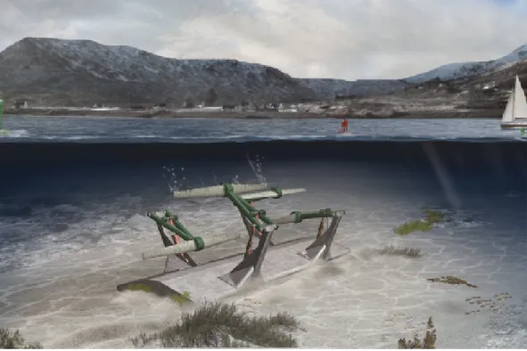
Figure 1.4: The 100 kW Pulse tidal oscillating wing device. Taken from [4]. The Pulse Tidal Ltd., England has developed two prototypes of oscillating wing turbine which feature two hydrofoils in a tandem configuration. The first prototype, depicted in Fig. 1.4, featured 100 kW of power and was deployed in the Humber estuary in 2009. The oscillating wing device has 12 m–long hydrofoils mounted on a marine platform. The second prototype, which is the largest known prototype so far, was installed in the Bristol Channel in 2014 and features rated power of 1.2 MW [17]. Figure 1.5 depicts the artistic impression of the Pulse Tidal oscillating wing device.
Another experimental prototype of the oscillating wing for power generation was designed, built and tested by Laval University in water at Lac–Beauport near Quebec
Figure 1.5: An artistic impression of the 1.2 MW Pulse Tidal oscillating wing device. Taken from [5].
City, Canada [6]. A 2 kW prototype included two aspect ratio (AR) 7 rectangular hydrofoils in a tandem configuration. Their tips featured endplates and the Reynolds number was 0.5 million. The coupling of the pitching and heaving motion of each hydrofoil is coupled through four–link mechanism. The turbine has been mounted on a pontoon boat and dragged on a lake, in order to be easily tested at various oper-ating conditions. Measured data reported fairly high values of the energy conversion efficiency. The experimental setup is depicted in Fig. 1.6.
1.2. Computational fluid dynamics for oscillating wing devices 6
Most recently Young et al.[17] published a comprehensive review of the analytical, numerical and experimental research work carried out in this field. The review also focuses on the influence of flapping kinematics and foil geometry parameter choice on the characteristics of the LEVS observed in certain operating conditions. This feature has been initially thought to have a beneficial effect on the efficiency of the energy generation of oscillating wings, and its analysis in realistic installations is one of the underlying threads of the present study. The authors of [17] also highlight outstanding questions on the fluid mechanics of the oscillating wing in real installations, charac-terised by relatively high values of the Reynolds number based on the foil chord and the freestream velocity, and complex 3D flow features. The kinematic set–ups of os-cillating wings for power generation can be subdivided in three classes [17, 18]: fully active, semi–passive and fully passive. In the fully active set–up all parameters of the heaving and pitching motions are prescribed; in the semi–passive set–up only the pitching motion is prescribed and the heaving motion parameters are determined by the hydrodynamic forces acting on the wing; in the fully passive arrangement, both the pitching and heaving motion parameters are determined by the forces acting on the wing. To date, it is still unclear which of the three set–ups provides the best perfor-mance [17], but progress made on improving the understanding of the hydrodynamic characteristics of any one of the three set–ups is likely to contribute to progress in the study and application of the other two [18]. The wing oscillation considered in most analyses is harmonic, but it has been shown that performance benefits can also be achieved by considering non–harmonic wing trajectories [19, 20]. The remainder of the literature survey in this subsection and the analyses in this work focus on the baseline configuration of the oscillating wing, namely that using a fully active kinematic set–up and harmonic wing motion.
Kinsey and Dumas [21] performed a thorough parametric computational fluid dy-namics (CFD) investigation into the dependence of the energy conversion efficiency of a foil oscillating in a laminar Reynolds 1,100–stream on the choice of motion parameters (heaving and pitching amplitude and motion frequency) and foil characteristic param-eters (foil thickness and location of pitching axis). Their study used the commercial CFD code FLUENT and concluded that, by suitably choosing motion frequency and pitching amplitude, efficiencies as high as 34 % could be obtained. They also reported that the main factor enabling this efficiency level is the achievement of an optimal synchronisation (or phase) of wing motion and unsteady LEVS associated with the dynamic stall observed for certain choices of foil trajectory parameters. The study also considers the detailed aerodynamic analysis of this device to better understand the inside of the complex unsteady aerodynamics mechanism, which controls the energy extraction process. The detailed flow analyses highlight the importance of the use of NS CFD for this application. Similar findings were also reported in a later independent study using the NS research code COSA [22].
Thereafter, the hydrodynamics of the devices tested at Lac–Beauport [6] was in-vestigated numerically by Kinsey and Dumas [23]. Both two–dimensional (2D) and three–dimensional (3D) turbulent FLUENT simulations using the Spalart–Allmaras turbulence model [24] were performed. The study highlighted that the loss of power generation efficiency of a single AR 7 wing with endplates in a water stream with
Re = 0.5×10⁶ is about 15 % of the efficiency of the infinite wing. In a follow–up
study, the same authors extended their numerical analyses to wings ofAR5, 7 and 10 with and without endplates to assess the dependence of the losses induced by finite– wing effects on aspect ratio and wing tip type setting again using Re = 0.5× 10⁶.
Making use of FLUENT simulations based on 3D grids with up to 3.5 million cells and using the Spalart–Allmaras model for the turbulence closure, their investigations
concluded that, for a finite wing ofAR≥10 with endplates such a loss could be limited to about 10 % of the efficiency of the infinite wing [25]. For the AR10 case, however, no simulation of the wing without endplates was performed, and therefore, it was not possible to assess separately the efficiency improvement due to the use of endplates and that due to the use of a fairly large and more realistic AR 10.
The dependence of the oscillating wing hydrodynamics on the Reynolds number is another crucial factor essential to maximising the energy extraction efficiency of future real installations. Cross–comparison of laminar low–Reynolds number and turbulent high–Reynolds number CFD simulations using the same wing motion parameters re-veals that such efficiency is significantly higher in the latter regime [21, 23, 26]. This was reported in [22], where COSA has been used to carry out a 2D fully laminar Reynolds 1,100–simulation and later on a 2D fully turbulent Reynolds 1.5 million– simulation [26] of the oscillating wing using the same wing motion parameters for both regimes. The comparative analysis reported in [26] used a wing trajectory that had been previously optimised for maximum energy extraction efficiency in the considered laminar regime, and provided two important observations. Firstly, the wing power generation efficiency increased at the turbulent high Reynolds number regime due pri-marily to thinner boundary layers, resulting in thinner effective foil and thus larger lift forces. Secondly, LEVS was delayed in the turbulent high Reynolds number regime with respect to the laminar low Reynolds number regime due to higher stability of the turbulent boundary layers. Thus the optimal synchronisation of wing motion and LEVS of the laminar regime was reduced in the high–Reynolds number case. However, the beneficial effect of thinner turbulent boundary layers outweighed the detrimental effect of abovesaid reduction of optimal synchronisation, resulting in higher efficiency of the foil in the turbulent stream. It was assumed that, for high Reynolds number regimes, resetting an optimal synchronisation of wing motion and LEVS by suitably varying the trajectory parameters could lead to an efficiency level even higher than that of 40 % obtained for the considered turbulent regime. However, Kinsey and Dumas later showed that high power generation efficiency at high Reynolds numbers does not necessarily rely on the occurrence of LEVS [27]. The detailed flow analyses of the 3D flow effects at realistic Reynolds numbers are still missing for this promising device, and will be addressed in this thesis.
1.3
Computational fluid dynamics for horizontal–
axis wind turbines
Wind turbine is defined as a device which harnesses the kinetic energy of the wind and converts it into mechanical work, which can then be used for electricity production. HAWT represent the most common design of the wind turbines. The production of the HAWT power mainly depends on the interaction between the wind turbine rotor and the wind. The aerodynamic blade forces, generated by the wind, determine the main characteristics of the wind turbine performance, such as the power output and loads [28].
In this work the aerodynamics of two HAWT rotors have been considered. Firstly, NREL Phase VI rotor is used for the validation of newly developed 3D predictive capabilities of CFD Optimised Structured multi–block Algorithm (COSA), in straight and yawed wind conditions, and also to explore how well the physics of this flow problem can be captured with a NS technology. NREL Phase VI experiment [9] features
1.3. Computational fluid dynamics for horizontal–axis wind turbines 8
many accurate and reliable measurements, and therefore represents a very suitable test case for CFD code validation. Secondly, the NREL 5–MW baseline turbine is herein used for the aerodynamic analyses in straight and yawed wind conditions. NREL 5–MW baseline fluid flow problem also serves the purpose of highlighting the high computational efficiency of the newly developed 3D HB solver in this research work.
Several other valuable experiments of the HAWT rotor aerodynamics have been conducted. One of the well known configurations is the MEXICO (Model Experi-ments in Controlled Conditions) experiment [29], which was designed to compliment the NREL Phase VI experiment [9]. However, for the purpose of this thesis only one validation test campaign was selected, which was the NREL Phase VI experiment.
1.3.1
NREL Phase VI wind turbine
NREL Phase VI wind turbine [9] has been developed in order to quantify the aero-dynamic behaviour and the flow three–dimensionality of the full scale HAWTs. The turbine was designed using low–fidelity design codes, which rely on aerodynamic forces based on the steady 2D wind tunnel airfoil test results. The experiment has highlighted that very strong 3D effects exist in the wind turbine field operation. The experiment has been conducted by the National Renewable Energy Laboratory (NREL) at the National Wind Technology Center (NWTC) near Golden, Colorado, USA. The wind tunnel used was that located at the NASA Ames Research Center at Moffett Field, Cal-ifornia, and has the size of 24.4m×36.6m. The experiments included both upwind and downwind configurations, as well as rigid and teetered. The test matrix also included various cone, blade tip pitch and yaw angles. The turbine was studied at rotating and parked conditions and for the different blade tip configurations. Many accurate and reliable quantitative aerodynamic and structural measurements on a Phase VI wind turbine have been acquired, therefore, these data are excellent for validation of CFD models for novel designs and analyses of advanced wind energy devices. For this thesis several measurements where the turbine was yawed to various angles are of particular importance.
The set of Phase VI experimental data has been used by many CFD studies, partic-ularly for the validation purposes. The test cases with the rotating blade at 72RP M
are usually considered at various wind velocities. One of the first numerical studies on Phase VI HAWT was a blind code study organised by the NREL [30], which in-cluded BEM models, prescribed wake models, free wake models and NS codes. The study has highlighted that the majority of the predicted data deviated quite a lot from the experimental data. The results suggested that a lack of high–fidelity models for accurately predicting the aerodynamic behaviour of the flow on the HAWT blades ex-ists. According to the NREL blind code comparison, Sørensen et al.have obtained one of the best overall agreement with the experimental data [31]. They have considered five operating conditions in straight wind, with the tip pitch angle 3◦, where only the rotor has been modelled. For their work, they have used EllipSys3D CFD code, which is a multiblock finite volume discretization of the incompressible Reynolds–Averaged Navier–Stokes (RANS) equations and thek−ωshear stress transport (SST) turbulence model. The agreement between the computed results and experimental data is quite good for most of the operating conditions, except for the operating point at the 10m/s, where the flow behaviour was very sensitive to the employed turbulence model.
Later on, Duque et al. [32] obtained a good agreement between the numerical and experimental data for the straight wind flow. They used compressible overset RANS code OVERFLOW–D2, and the 1–equation Baldwin–Barth turbulence model. They
also compared RANS CFD calculations with a vortex lattice code CAMRAD II, and came to the conclusion that overall, the CFD calculations show much better agreement with the experimental data. The OVERFLOW–D2 is capable of predicting the stalled flow conditions, whereas the CAMRAD II code fails to accurately predict the stalled flow conditions.
Le Pape et al. [33] have conducted their work on Phase VI, as a continuation of previous numerical studies of Sørensen et al. and Duque et al. [31, 32]. They have used the compressible RANS solver ELSA with the k−ω SST turbulence model. The detailed flow analysis of the 3D and unsteady flow effects have been conducted for the zero–yaw configuration, for various numbers of operating conditions. The obtained results were in a reasonable agreement with the experimental data, however, it was suggested that the usage of the low speed preconditioning will most likely improve the results for a compressible NS solver. Later on Le Pape et al. [33] conducted the calculations for both the straight and 10◦ yawed wind flow, with the usage of the low speed preconditioning [34]. This study has shown that a low speed preconditioner indeed improves the accuracy of the results at low wind speeds and allows better prediction of the stall point.
Due to the popularity of this test case for code validation, and further aerodynamic analyses, more recent studies have followed. Gómez–Iradiet al.[35] performed analyses using the compressible NS solver with the k−ω SST turbulence model. Overall good agreement between the numerical and experimental data has been obtained. This study has also taken into the account the effect of the wind–tunnel wall effects on the blade aerodynamics, and investigated the blade/tower interaction. Yu et al. [36] conducted a study on the overpredicted lift and stall delay of straight wind calculation, using the incompressible RANS solver with the k − ω SST turbulence model with transition correction. Stall delay is a condition, where the AoA at which stall occurs is greater for a rotating blade compared to static airfoil. The study has confirmed there is a stall delay phenomenon in the inboard part of the turbine blade. The NS results were compared with the experimental data and the lifting surface method with and without Du–Selig stall delay model. The NS results for low–speeds are in good agreement with the experimental data, however, at relatively high wind speed (10m/s), when the massive flow separation occurs, some discrepancy between the numerical and experimental data exists. Lifting surface method with Du–Selig stall delay model agrees well with the experimental data, whereas, without Du–Selig model it fails to accurately predict wind turbine performance. Another study, performed by Moshfeghi et al.[37], investigated the effects of near–wall grid spacing and aerodynamic behaviour of Phase VI blade using Ansys–CFX11 and thek−ωSST turbulence model. The study reports that in order to obtain grid–independent solution, presently used 5 million cell grids, would require more refinement in both chordwise and spanwise directions. Furthermore, the authors show there is a significant dependence of computed forces on near–wall spacing. Moreover, the results indicate that thek−ω SST turbulence model mispredicts separation point, and over predicts separation. Yu et al. [38] examined the rotor under the yawed flow conditions for two yaw angles of 30◦ and 60◦ for three wind speeds of 7, 10 and 15m/s. The unstructured incompressible RANS solver with the k−ω SST and correlation–based transition turbulence model has been used. The study reports that the blade aerodynamic loading is significantly reduced under the yawed wind flow. An overall good agreement between the numerical and experimental data for all wind speeds has been observed.
1.3. Computational fluid dynamics for horizontal–axis wind turbines 10
1.3.2
NREL
5
–MW baseline wind turbine
NREL offshore 5–MW baseline wind turbine, is a virtual model of a modern commercial three–bladed upwind variable–speed variable blade–pitch–to–feather–controlled tur-bine, developed at NREL [39]. The initial purpose of the turbine has been to establish the reference specifications for a number of research projects supported by the U.S. DOE’s Wind & Hydropower Technologies Program [39]. However, since the NREL offshore 5–MW baseline wind turbine has been adopted as a reference model by Union UpWind research program and the IEA Wind Annex XXIII Subtask 2 Offshore Code Comparison Collaboration (OC3), the model has been used as a reference by many research teams worldwide, for various different purposes. The aim of this model is to standardise onshore and offshore multimegawatt turbine specifications, and to quantify the benefits of advanced onshore and offshore wind energy technologies.
Sørensen and Johansen [40] have performed the NREL 5–MW baseline rotor calcu-lations in zero yaw wind for the uniform inflow and atmospheric boundary layer cases. The purpose of the study was to investigate the unsteady effects due to the severe vertical shear, and to compare the agreement with the BEM code. The calculations were performed using an incompressible NS CFD code EllipSys3D using thek−ω SST turbulence model. Later on, Chow and van Dam [41] have investigated the aerody-namic characteristics of the NREL 5–MW baseline rotor, using the compressible NS code OVERFLOW2 featuring the k −ω SST turbulence model. The study reports that the significant radial flow and inboard blade separation exist, and can be limited using various passive geometric modifications, resulting in improved power prediction. Additionally, it was concluded that the increasing inboard blade twist does not have a beneficial effect on power production. This study also compared the CFD results obtained by the incompressible CFD code EllipSys3D, reported by Sørensen and Jo-hansen in [40], and BEM predictions. The two CFD results at low wind velocities are in excellent agreement. However, once the rated power is reached, OVERFLOW2 predicts slightly higher power with respect to the EllipSys3D solutions. Before the rated speed, BEM predictions match well with both CFD codes. However, after the rated speed is achieved, the BEM analyses significantly overpredict the result of both CFD codes. Chow and van Dam’s study was further extended in [42], where a com-prehensive near–body grid independence study has been performed. It was found that the solution strongly depends on the near–body wake grid refinement, as the rapid diffusion of the wake in case of insufficient refinement contributes to the overpredicted torque and thrust. Chow and van Dam have performed another study on the NREL 5–MW baseline rotor [43], where they investigated the impact of the blade twist and blunt trailing–edge in the inboard region of the blade on the aerodynamic performance. They concluded that decreasing the sectional twist angle, which increases the sectional AoA, causes deeper stall of the inboard region of the blade, keeps the rotor torque constant and increases the thrust. Whereas, when increasing the sectional twist angle, the rotor thrust drops at faster pace than the torque, which could potentially lead to a more optimal designs in terms of the torque versus thrust ratio. Furthermore, it is also reported that the twist distribution of the NREL 5–MW baseline rotor is already nearly optimal. Moreover, the study pointed out that the blunt trailing edge modifications in the inboard part of the blade have a positive effect on the turbine performance, and completely change the flow behaviour. Chow and van Dam also pointed out that only high–fidelity 3D simulations are able to accurately predict the flow field of the modern rotor designs, due to their geometric complexity.
Troldborget al.[44] investigated the wake of the NREL 5–MW baseline rotor, using the incompressible EllipSys3D NS code, either using thek−ω SST or the DES version
![Figure 1.2: Side view of the oscillating–wing hydropower generator. Taken from [2].](https://thumb-us.123doks.com/thumbv2/123dok_us/1882761.2774828/24.892.222.779.807.1102/figure-view-oscillating-wing-hydropower-generator-taken.webp)
![Figure 1.4: The 100 kW Pulse tidal oscillating wing device. Taken from [4].](https://thumb-us.123doks.com/thumbv2/123dok_us/1882761.2774828/25.892.246.756.512.904/figure-kw-pulse-tidal-oscillating-wing-device-taken.webp)