Potravinarstvo Slovak Journal of Food Sciences vol. 12, 2018, no. 1, p. 472-486 doi: https://doi.org/10.5219/865
Received: 8 January 2018. Accepted: 6 May 2018. Available online: 29 May 2018 at www.potravinarstvo.com © 2018 Potravinarstvo Slovak Journal of Food Sciences, License: CC BY 3.0
ISSN 1337-0960 (online)
SOFTWARE SUPPORT FOR COST CALCULATION – APPLICATION TO THE
AGRICULTURAL SECTOR
Lenka Hudáková Stašová
ABSTRACT
Calculation of product costs is the source of information on the costs of selected produced products with great explanatory power. In current practice, the overhead costs on farms are monitored and calculated by species. They are allocated using an allocation base (average state of the animals, harvested area in hectares) or are converted using direct costs of the activity as an allocation base. With the current high level of overheads, this method cannot be considered effective. Only type classifications are monitored and are therefore anonymous in relation to activities. We consider high overhead costs as a good reason for implementing and using the methods of Activity Based Costing. In this paper we present a proposed model of Activity Based Costing for its use in agriculture, created in MS Excel. We create the model as a basic version, which can be more closely defined depending on the particular conditions of the business implementing the model. We complete the general model for better illustration with figures on costs. We present a comparison of model results with the traditional approach of calculating costs in agriculture. One of the biggest benefits of the ABC system is the binding of costs from accounts, activities performed and the cost of products in one system. We present a statistical comparison of model results with the traditional approach of calculating costs in agriculture.
Keywords: traditional cost calculation; Activity Based Costing method; agricultural business; Activity Based Costing model; controlling
INTRODUCTION
Information is a prerequisite for any management activity. Its value is growing continuously. Objectively, rapidly and correctly addressed information inside the company is an important basis for its effective
management. One requirement is more accurate
calculations of product costs. Clarification involves removing differences in the allocation of overhead costs and the replacement of a distorted image with a true picture based on the causal connections arising from real resource consumption.
Calculation of product costs is an important part of the company’s information system (Tóth et al., 2016). It is the source of information on the costs of selected produced products with great explanatory power (Kubicová and
Habánová, 2016).
At present, agriculture in the Slovak Republic mainly uses traditional methods for the calculation of production costs. Traditional calculation formulas work with overheads (as opposed to modern methods of calculations that convert non-specific, anonymous overheads into direct costs). Traditional calculations do not reflect the needs of the market environment.
The agricultural sector is characterized by a high proportion of overheads. These are costs that cannot or would not be economical to monitor by calculation unit
(Ferenczi-Vaňová et al., 2017). Overhead costs are therefore indirectly reflected in product costs of calculation units through an allocation base. The allocation base used is the direct costs of the different crops grown, animals raised, customer orders, work and services for others.
Managing overhead costs is complicated and therefore each business should try, in calculating production costs, to place the most costs directly on a calculated product or activity as direct costs. Therefore, it is necessary to change the content structure of individual cost items of the calculation formula. A good solution to the problems in overhead costs is non-traditional methods of calculating production costs, in particular ABC (Activity Based Costing), which brings a new perspective on overheads and turns them into direct costs.
The importance of the ABC calculation method is summarized in the following literature review.
According to Kaplan and Anderson (2003, 2005, 2007)
Activity Based Costing is an approach to solve the problems of traditional cost management systems. These
traditional costing systems are often unable to determine accurately the actual costs of production and of the costs of related services. Consequently managers were making decisions based on inaccurate data especially where there are multiple products. Instead of using broad arbitrary percentages to allocate costs, ABC seeks to identify cause and effect relationships to objectively assign costs. Once costs of the activities have been identified, the cost of each activity is attributed to each product to the extent that the product uses the activity. In this way ABC often identifies areas of high overhead costs per unit and so directs attention to finding ways to reduce the costs or to charge
more for costly products (Chrenková, 2011;
Cannavacciuolo et al., 2015; Duh et al., 2009). In present
day manufacturing organizations, performance
measurements play an important role in providing strategic directions and developing corresponding operational policies and methods. One such method is the activity‐based costing (ABC) method which calculates the cost of activities and helps in making decisions on product mix and price for improving the utilization of resources and minimizing the cost of production (Ittner et al., 2002; Quinn et al., 2017). Even now some manufacturing
organizations employ traditional costing methods
depending upon their market forces and characteristics. One of the most important decisions to be made is about the type of costing system that would be suitable for an organization (Slangen et al., 2003; Zhang et al., 2015). The role of direct labour in current manufacturing environments has diminished, but at the same time the level of support services has increased. Traditional methods of cost calculation do not take into account this increased complexity and still allocate overhead costs by their diminishing labour base or even do not take into
account overhead costs (Gunasekaran, et al., 1999;
Kostakis, H., 2008).
Veščičík (2004, 2012) explains that Activity Based Costing is a new modern method of calculating the cost of individual processes, products and customers, which eliminates the inaccuracies of traditional methods of the last century (overhead calculations, covering post). Traditional cost accounting methods were developed at a time when direct costs of labour and material factors of production were dominant and when changes in technology and consumer demand were not so fast
(Gunasekaran et al., 1999; Kaszubski and Ebben, 2005; Kostakis, 2008). The problems with traditional cost accounting emerge when indirect costs (such as maintenance, insurance, production preparation, etc.) amount to significant sums or are even higher than direct costs. Activity Based Costing is a commonly used tool and has practical significance for the specific conditions of agricultural production, where it can be used to achieve the
improvement of cost management (Zakić, Borović, 2013;
Kaszubski and Ebben, 2005; Khataie and Bulgak, 2013). Activity Based Costing represents a universal management instrument that is used not only for the purposes of cost calculations, but represents a tool enabling effective cost reduction. In addition to these advantages, the ABC method has also its restriction as it is more demanding in terms of the volume and structure of the data processing. In case of its application, it is therefore necessary to consider carefully all the benefits
and costs associated with its implementation (Popesko, 2010, 2012; Popesko et al., 2015).
Pokorná (2016) states that looking for factors affecting business performance is one of a central concern of business economists for several years. Activity-Based Costing (ABC) is a management tool that provides additional and more accurate information on the costs and company performance, thus contributes to better manager decision making, and thus has potential to affect the financial performance. The ABC expansion among enterprises in the Czech Republic is currently comparable with neighbouring countries, although the extent of its use is lower.
The extensive ABC use is associated with higher quality levels and greater improvements in cycle time and quality, and is indirectly associated with manufacturing cost reductions through quality and cycle time improvements
(Krumwiede and Charles, 2014; Lelkes, 2014). However, on average, extensive ABC use has no significant association with return on assets. Instead, weak evidence that the association between ABC and accounting profitability is contingent on the plant’s operational characteristics (Ittner et al., 2002; Dalci et al, 2010; Kuethe and Morehart, 2012). An Activity Based Costing system is a system that focuses attention on the costs of various activities required to produce a product or service
(Langfield-Smith et al., 1998; Jánsky et al., 2012). The ABC method is a progressive instrument of controlling. It enables to assign costs to products according to actually used up activities and resources. The method is designed for more accurate scheduling of indirect costs (overheads); as a schedule using the causal relationship between
activities (processes) and individual performance.
(Foltínová, 2011). The main principle of the ABC is placing the activities among the source costs (taken over from the accountancy) and the products. One of the biggest benefits of the ABC system is the interconnection of the costs arising from the accounting, processes and costs of products into one system (Veščičík, 2012; Greasley and
Smith, 2017).
Cohen et al. (2005) present evidence that the possibility of future ABC adoption is related to the degree of satisfaction from the currently used cost accounting system. Companies that do not intend to adopt ABC (ABC deniers) were found to be more satisfied with their existing cost accounting system in comparison to ABC supporters. They also report the characteristics of companies that still have complete ignorance of the ABC technique (ABC unawares).
Following the above, the paper is divided into three parts. The first part presents a theoretical overview of calculation methods in agriculture, defines the specifics of agriculture and also presents an overview of opinions on the importance of the ABC method. The second part is devoted to the creation and implementation of a calculation model created by ABC method (non-traditional method for agriculture). The third part is focused on the statistic analyses and comparing the traditional calculation method with the ABC method.
Scientific hypothesis
The aim of this paper is to create a proposal for implementation of Activity Based Costing, which is also
supported by the developed software solution design in MS Excel.
MATERIAL AND METHODOLOGY
The result is the presented methodology for calculating Activity Based Costing, which is based on a model in MS Excel 2013 and takes into account the specifics of primary agricultural production. The calculation model is created in the spreadsheet Microsoft Office Excel 2013 from the company Microsoft for the operating system Microsoft Windows and Macintosh, version number 15.0.4535.1511. The presented model of implementation of ABC is designed as a framework proposal in generic agriculture companies, supplemented in the paper with real data and then calculated results.
In order to achieve the aim of this paper, we analyse the current state of costs calculated in agriculture, then we define the specifics of primary agricultural production, particularly in conditions of transition economies. In the next part of the article, we specify the main activities in the production processes of crop and livestock production as a prerequisite for the use of the Activity Based Costing method in the structure of the calculation information system. Specification of activities focuses mainly on overhead costs for major production (crop and livestock) and administrative expenses, but also on the field of auxiliary production. These activities are specified in a selected agricultural cooperative, with the fictitious name Agroprodukt. For analysis of performance in crop production, we work with the products of wheat, barley, sugar beet, corn for grain and livestock production with products of milk cows- milk, fattening beef cattle, fattening pigs, fattening chickens.
From a methodological point of view, we use the non-traditional calculation method, Activity Based Costing, which charges all the indirect costs first to activities because they cause the need for costs and then divides activities to products, because products cause the need for the implementation of activities. This new view of costs enables their cost and complexity to be assessed compared with their benefits, creating a natural pressure to eliminate activities that are not effective.
The principle of the ABC method lies in the fact that in the first step the direct costs are assigned to outputs (this method does not bring anything new) and indirect (overhead) costs are assigned to activities (this is a substantial change). In the second step, the activities are assigned to individual cost items according to their degree of load of consumption for the activities necessary for their provision. Unlike the traditional approach – "everything to everyone equally" a selective system is applied on the basis of actual causation, that is, "to each only what they really consume, or what is consumed because of them." When implementing the ABC method in the selected enterprise, we follow generally defined steps to implement this method: a preparatory phase, specification of activities, aggregation of activities, identification of activity centres, first stage of allocation – costing of activities, creating the structure of the flow of costs, goods and identification of the activity centres, specification of products, the second stage of allocation – calculation of the cost of products, evaluation of results. Attention is paid to the selection and calculation of drivers.
For the purpose of comparison, the traditional method of calculation of product costs will be used with an allocation base formulated in the analysed fictional company. The principle of the traditional calculation methodis that we use the same allocation base for all kinds of overheads. Direct costs are allocated directly to the product, as is the case with the ABC method. It is used direct labour costs or total direct costs as an allocation base. For example - the percentage assignment of overhead costs to individual products is calculated: overhead / direct labour costs. The material for analysis is the data on the levels of cost items found in the analysed company. The starting data sources for creation of the entire model are costs by type (reported in Table 2).
Subsequently, we have established a scientific
hypothesis: Cost calculation using the traditional calculation method (based on the allocation base) is less accurate, distortive compared to cost calculation by the ABC method.
-H0: Equation of the mean values for both methods. -H1: Inequality of the mean values for both methods. In order to perform the statistical analysis, we used the real data of 22 agricultural enterprises (Grange, Ltd., SpA.). This is partly the data of companies that have already implemented the ABC method, in part data on enterprises that use only the traditional approach and the ABC method was modelled them (5 of these enterprises we modelled on ourselves, we obtained the rest of the data
from consulting companies dealing with ABC
implementation in enterprises).
Since the ABC method does not bring anything new in the direct cost allocation (allocates them directly to the product as a traditional approach), we included in the statistical analysis only the amount of overheads. These calculation approaches allocate overheads differently. The aim is to confirm or refute the established hypothesis. We perform tests of normality, we tested normality with two tests: Kolmogorov-Smirnov test and Shapiro-Wilk test (Table 7). We evaluate data statistically using a paired t-test (Paired Samples Test), we evaluate the p-value (Table 8).
Statisic analysis
In statistics, the Kolmogorov–Smirnov test (K-S test or KS test) is a nonparametric test of the equality of continuous, one-dimensional probability distributions that can be used to compare a sample with a reference probability distribution (one-sample K-S test), or to compare two samples (two-sample K-S test).
The Kolmogorov-Smirnov statistic quantifies a distance between the empirical distribution function of the sample and the cumulative distribution function of the reference distribution, or between the empirical distribution functions of two samples. The null distribution of this statistic is calculated under the null hypothesis that the sample is drawn from the reference distribution (in the one-sample case) or that the samples are drawn from the same distribution (in the two-sample case). In each case, the distributions considered under the null hypothesis are continuous distributions but are otherwise unrestricted. The Shapiro-Wilk test is a test of normality in frequentist statistics. The test rejects the hypothesis of normality when the p-value is less than or equal to 0.05. Failing the
normality test allows you to state with 95% confidence the data does not fit the normal distribution. Passing the normality test only allows to state no significant departure from normality was found.
A t-test is appropriate for comparing means under relaxed conditions (less is assumed).
Paired tests are appropriate for comparing two samples where it is impossible to control important variables. Rather than comparing two sets, members are paired between samples so the difference between the members becomes the sample. Typicaly the mean of the differences is then compared to zero. The common example scenario for when a paired difference test is appropriate is when a single set of test subjects has something applied to them and the test is intended to check for an effect.
We established suitable null and alternative hypostheses: Null Hypothesis H0: μ = μ0
Alternate Hypothesis H1: μ >μ0 We used four steps, listed below: 1. Calculate the sample mean.
2. Calculate the sample standard deviation. 3. Calculate the test statistic.
4. Calculate the probability of observing the test statistic under the null hypothesis. This value is obtained by comparing “t” to a t-distribution with (n − 1) degrees of freedom.
The test is based on the differences of the measured pair
values in the compared variation ranges. We test the hypothesis that the mean value of the traditonal calculation method and non - traditional method equals (or: the difference of the mean values of the pair measurements is zero).
First, we calculate the pair differences of the sample (n -
number of pairs) and calculate the arithmetic mean and
the standard deviation "s" (or the variance s2) from the differences found.
Then we calculate test criterion (statistics) t:
The p-value (probability value) for the t-statistic is „p“:
p = 2 . Pr(T >|t|) (two-tailed) p = Pr(T >t) (upper-tailed) p = Pr(T <t) (lower-tailed)
determine whether the results provide sufficient evidence to reject the null hypothesis in favor of the alternative hypothesis.
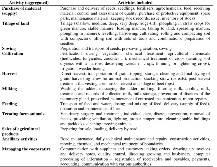
Table 1 Specification of activities and their aggregation.
Activity (aggregated) Activities included
Purchase of material (supply)
Purchase and delivery of seeds, seedlings, fertilizers, agrochemicals, feed, receiving material, control and assessment of quality, purchase of protective equipment, spare parts, maintenance material, keeping stock records, issue, inventory of stocks
Tillage of land Tillage (shallow, medium, deep, very deep, ridge-till), ploughing in straw crops for green manure, stable manure (loading manure, taking to land, spreading manure, ploughing in manure), levelling, harrowing, cultivating, rolling and compacting soil with compactors, tilling soil with sets of tools and combinations, preparation of seedbed
Sowing Preparation and transport of seeds, pre-sowing aeration, sowing
Cultivation Fertilization during vegetation, chemical treatment agricultural chemicals (herbicides, fungicides, zoocides ...), mechanical treatment of crops (aerating soil dryness with a harrow, destroying weeds in crops, thinning or lightening crops), irrigation, weeder-hoeing
Harvest Direct harvest, transportation of grain, tipping, storage, cleaning and final drying of grain, harvesting straw for animal production, stacking straw (cereals), post-harvest treatment (harvesting corn husks, harvest and silage of beet tops)
Milking Washing the udder, massaging the udder, milking, filtering milk, cooling milk, treatment and records of collected milk, milk storage, prevention of diseases of the mammary gland, prescribed maintenance of entrusted mechanization, minor repairs
Feeding Transport of feed and water, dosing and mixing of feed, delivery (supply of feed), operation and maintenance of lines
Treating farm animals Veterinary surgery and treatment, individual care, disease prevention, removal of faeces, providing ventilation, lighting, proper temperature, cleaning stable buildings and paddocks, cleaning, moving animals
Sales of agricultural products
Preparing for sale, loading, delivery by road
Ancillary activities Road maintenance, daily technical maintenance and repairs, construction activities, mowing, chemical and mechanical treatment of boundaries
Managing the cooperative Communication with suppliers and customers, taking orders, drawing up invoices and delivery notes, quality control, directing growing and husbandry, computer processing of information – registration of receivables and payables, payments, accounting, communication with various authorities
RESULTS AND DISCUSSION
Defining the specifics of agriculture in creating a
proposal for implementation of the ABC method
The level of costs for agricultural products and their calculation, as distinct from other sectors of the national economy, is influenced by other factors resulting from the character of agricultural production. Among the most important are:
Natural factors, particularly in crop production – this includes soil conditions, weather conditions and the position of the land.
High consumption of own products in the production process - in-house consumption, due to the overlap between crop and livestock production.
Fragmentation of land and its shape – negative influence on the transport costs and labour costs for mechanized work in crop production.
Cycle of current assets. Affects development costs and their reproduction with inequality during the calendar year (accounting, tax year). Crop production takes a year; in most sectors of animal production it is longer than a year. Industry, to an ever greater extent, decides about the level of costs (range, quality of agricultural inputs).
In agriculture, there is some damage that directly or indirectly affects costs (death of animals, frost of winter crops, destruction of the plants by floods, droughts, pests, etc.).
When drawing up the proposal for implementation of the ABC method it is necessary to take these specifications into account, because of their impact on the method of calculating costs. Taking into account the overlap between crop and animal production enables the capture of the
production process, regardless of the length of the production cycle and enables activity in the manufacturing process to be recorded in such a way that it is possible to attribute costs to them in causal relationship.
Besides these general specifics of agriculture, it is necessary in transition economies to consider other factors, particularly limited financial resources, poor technical equipment of the business, using the traditional system of management accounting and calculations, not least the distrust of workers towards everything new and unusual. Therefore, for an agricultural company, low financial requirements for software are important. To avoid the mistrust of workers, the simplicity of the model of Activity Based Costing and logical clarity of its individual components is important, as is the ease of use.
Proposal of implanting the model and application
in MS Excel suitable for agricultural businesses
While creating the proposed model of ABC we apply the procedures described in the methodological part of the paper.
In the studied agricultural cooperative, Agroprodukt, we specified activities and linked them to the activities listed in Table 1. We selected basic activities related to production of eight products for which we are calculating the cost in the proposed model. The ABC method is intended primarily for the allocation of overhead costs. When specifying activities it is therefore necessary to maintain a balanced level of detail and not to confuse this phase of implementation with defining the technological standards and manufacturing processes. Specification of activities is a precondition for applying the ABC method.
Table 2 CostData sheet.
COSTS Total costs in €
Consumed material
Fuels, oils and lubricants 15 000
Protective equipment 833
Cleaning and small material for maintenance of buildings and structures for animal
production 5 833
Material for maintenance of office buildings 500
Material for the daily technical maintenance and repairs 3 167
Consumption of drugs and disinfectant material 1 500
Consumed energy 2 167
Consumption of other non-inventory items
Water 8 500
Wages and salaries
Payroll management 17 333
Wages for the daily technical maintenance and repairs 16 333
Amortization of long-term intangible assets and depreciation of long-term tangible
assets
Harvesters and tractors, self-propelled machines, tensioning system 21 667
Office buildings and warehouses 9 000
Single-purpose buildings and facilities for animal production 19 333
Machines and mechanisms in animal production 10 667
Trucks 10 333
Cars 8 500
Equipment of office buildings 6 333
Other operating expenses 12 667
Running costs of buildings (insurance, real estate tax, cost of heat) 15 167
The tax on agricultural land 15
Table 3 CostAllocation-1stStage sheet (Table A, Table B, Table C).
A Relationships between costs and activities
COSTS ACTIVITIES
A1 A2 A3 A4 A5 A6 A7 A8 A9 A10 A11
Consumed material
Fuels, oils and lubricants X X X X X X X X X
Protective equipment X X X
Cleaning and small material for maintenance of buildings and
structures for animal production X X X
Material for maintenance of office buildings X
Material for the daily technical maintenance and repairs X
Consumption of drugs and disinfectant material X
Consumed energy X X X
Consumption of other non-inventory items
Water X X X
Wages and salaries
Payroll management X
Wages for the daily technical maintenance and repairs X
Amortization of long-term intangible assets and
depreciation of long-term tangible assets
Harvesters and tractors, self-propelled machines, tensioning
system X X X X X
Office buildings and warehouses X X
Single-purpose buildings and facilities for animal production X X X
Machines and mechanisms in animal production X X
Trucks X X X X X
Cars X
Equipment of office buildings X
Other operating expenses X
Running costs of buildings (insurance, real estate tax, cost of
heat) X X X
The tax on agricultural land X X X X
Cost of vehicles X X X
B Cost drivers of the 1st stage COSTS Total costs in € Total value of driver ACTIVITIES A1 A2 A3 A4 A5 A6 A7 A8 A9 A10 A11 Consumed material
Fuels, oils and lubricants 15 000 100% 8 19 11 7 17 6 11 9 12 Protective equipment 833 100% 20 20 60 Cleaning and small material for
maintenance of buildings and structures for animal production
5 833 100% 33.3 33.3 33.3
Material for maintenance of office
buildings 500 100% 100
Material for the daily technical
maintenance and repairs 3 167 100% 100 Consumption of drugs and disinfectant
material 1 500 100% 100
Consumed energy 2 167 100% 35 45 20
Consumption of other non-inventory
items
Water 8 500 100% 30 20 50
Wages and salaries
Payroll management 17 333 100% 100 Wages for the daily technical
Amortization of long-term intangible assets and depreciation of long-term tangible assets
Harvesters and tractors, self-propelled
machines, tensioning system 21 667 100% 25 20 15 25 15 Office buildings and warehouses 9 000 1150m2 900 250 Single-purpose buildings and facilities
for animal production 19 333 100% 33,3 33,3 33,3 Machines and mechanisms in animal
production 10 667 100% 50 50
Trucks 10 333 100% 15 10 30 25 20
Cars 8 500 100% 100
Equipment of office buildings 6 333 100% 100
Other operating expenses 12 667 100% 100
Running costs of buildings (insurance,
real estate tax, cost of heat) 15 167 1850m2 900 655 250 The tax on agricultural land 15 100% 25 25 25 25 Cost of vehicles 6 000 100% 30 30 40 C Costs of activities COSTS Total costs in € ACTIVITIES A1 A2 A3 A4 A5 A6 A7 A8 A9 A10 A11 Consumed material
Fuels, oils and
lubricants 15 000 1 200 2 850 1 650 1 050 2 550 900 1 650 1 350 1 800 Protective
equipment 833 166.5 166.5 500
Cleaning and small material for maintenance of buildings and structures for animal production 5 833 1 944.33 1 944.33 1 944.33 Material for maintenance of office buildings 500 500
Material for the daily technical maintenance and repairs 3 167 3 167 Consumption of drugs and disinfectant material 1 500 1 500 Consumed energy 2 167 758.5 975.1 433.4 Consumption of other non-inventory items Water 8 500 2 550 1 700 4 250 Wages and salaries Payroll management 17 333 17 333
Wages for the daily technical maintenance and repairs 16 333 16 333 Amortization of long-term intangible assets and depreciation of long-term tangible assets Harvesters and tractors, self-propelled machines, tensioning system 21 667 5 416.75 4 333.4 3 250 5 416.75 3 250 Office buildings and warehouses 9 000 7 043.50 1956.5
After specification of activities we can proceed to the actual cost calculation, which takes place in two steps. For creating a model in Excel, it is important that the agricultural businesses have the opportunity to export the data from accounting software to MS Excel. After talking with the workers from consulting software companies, we found that at least in a basic form, this is also possible for older accounting software.
We create the proposed model in MS Excel. In the file
we created individual sheets as needed for implementation
methods in the agricultural firm: CostData,
CostAllocation-1stLevel, CostFlowStructure,
CostAllocation-2ndLevel. On each sheet there are tables needed for calculations using the ABC method. Consequently, we defined the links between cells and sheets. Models are like the basic version, which can be adjusted accordingly to the needs of the business. The general model is completed with data on costs for better
Single-purpose buildings and facilities for animal production 19 333 6 444.33 6 444.33 6 444.33 Machines and mechanisms in animal production 10 667 3 333.50 3 333.50 Trucks 10 333 1 550 1 033.33 3 100 2 583.20 2 066.50 Cars 8 500 8 500 Equipment of office buildings 6 333 6 333 Other operating expenses 12 667 12 667 Running costs of buildings (insurance, real estate tax, cost of heat) 15 167 7 562.40 5 503.70 2 1006 0 The tax on agricultural land 15 115 115 115 115 Cost of vehicles 6 000 1 800 1 800 2 400 Total costs 190 848 19 155.90 8 270.5 7 020.5 7 020.2 11 070.50 16 180.66 21 455.36 16 534.26 5 516.5 24 600 54 023.5
Source: own software program.
Table 4 CostFlowStructure sheet (Table A, Table B, Table C, Table D, Table E).
A Relationships between activities
COSTS Total
costs in €
ACTIVITIES
A1 A2 A3 A4 A5 A6 A7 A8 A9 A10 A11
Consumed material
Fuels, oils and lubricants 15 000 1 200 2 850 1 650 1 050 2 550 900 650 1 1 350 1 800
Protective equipment 833 166.5 166.5 500
Cleaning and small material for maintenance of buildings and structures for animal production
5 833 1 944.33 1 944.33 1 944.33
Material for maintenance of office buildings 500 500 Material for the daily technical maintenance
and repairs 3 167 3 167
Consumption of drugs and disinfectant
material 1 500 1 500
Consumed energy 2 167 758.5 975.1 433.4 Consumption of other non-inventory items
Water 8 500 2 550 1 700 4 250
Wages and salaries
Payroll management 17 333 17 333
Wages for the daily technical maintenance and
repairs 16 333 16333
Amortization of long-term intangible assets and depreciation of long-term tangible assets
Harvesters and tractors, self-propelled
machines, tensioning system 21 667 5 416.75 4 333.40 3 250 5 416.75 3 250 Office buildings and warehouses 9 000 7 043.50 1956,5 Single-purpose buildings and facilities for
Machines and mechanisms in
animal production 10 667 3 333.50 3 333.50
Trucks 10 333 1 550 1 033,33 3 100 2 583.20 2 066.50
Cars 8 500 8 500
Equipment of office buildings 6 333 6 333
Other operating expenses 12 667 12 667
Running costs of buildings (insurance, real estate tax, cost of heat)
15 167 7 562.40 5 503.70 2 100.60
The tax on agricultural land 15 115 115 115 115
Cost of vehicles 6 000 1 800 1 800 2 400
Total costs 190848 19 155.90 8 270.50 7 020.55 7 020.25 11 070.50 16 180.66 21 455.36 16 534.26 5 516.50 24600 54 023.50
B Distribution of the costs of activity No.11
ACTIVITIES Total costs ACTIVITIES A1 A2 A3 A4 A5 A6 A7 A8 A9 A10 A11 Total costs 19 155.90 8 270.50 7 020.55 7 020.25 11 070.50 16 180.66 21 455.36 16 534.26 5 516.50 24 600 54 023.50 A1 19 155.90 A2 8 270.50 A3 7 020.55 A4 7 020.25 A5 11 070.50 A6 16 180.66 A7 21 455.36 A8 16 534.26 A9 5 516.50 A10 24 600.00 A11 54 023.50 14 025 1 793 3 188.50 3 748 5 465 2 245 4 133 3 319 11 582 4 525 Total costs 190 848 33 180.90 10 063.50 10 209.05 10 768.25 16 535.50 18 425.66 25 588.36 19 853.26 17 098.50 29 125
C Distribution of the costs of activity No.1
ACTIVITIES Total costs ACTIVITIES A1 A2 A3 A4 A5 A6 A7 A8 A9 A10 A11 Total costs 33 180.90 10 063.50 10 209.05 10 768.25 11 070.50 18 425.66 25 588.36 19 853.26 17 098.50 29 125 A1 33 180.90 11 405.50 14 581 7 194.40 A2 10 063.50 A3 10 209.05 A4 10 768.25 A5 11 070.50 A6 18 425.66 A7 25 588.36 A8 19 853.26 A9 17 098.50 A10 29 125.00 A11 Total costs 190 848 10 063.50 21 614.55 10 768.25 16 535.50 18 425.66 40 169.36 19 853.26 17 098.50 36 319.40
D Distribution of the costs of activity No.10
ACTIVITIES Total costs ACTIVITIES
A1 A2 A3 A4 A5 A6 A7 A8 A9 A10 A11
illustration.
The CostData sheet (Table 2) contains items from cost accounts in their detailed analytical breakdown. They are exported from the accounts of the company. This sheet serves as the source data for further sheets of the program. The CostAllocation-1stStage sheet (Table 3) performs the first step in the cost allocation model. It contains three tables. Table A is necessary to define relationships between costs and activities by constructing a matrix of dependency. If activity "i" causes the formation of cost "j", the cell "i.j" is filled in with "X". After recording all the relationships between the activities and costs of the analysed agricultural cooperative we can determine which activities consume various costs. In table B it is necessary to define the cost drivers of the 1st stage on the basis of correlation between the costs and activities. They are used for the first stage of allocation, i.e. allocation of costs to individual activities. In practice, it often happens that cost drivers need to be a qualified estimate. It is necessary to define the percentage of the cost of individual activities, either on the basis of technological intensity, growing share in crop production or under otherwise specified criteria. It is important that this part of created model has been subject to consultation with the workers who are directly involved in an activity or workers who have information about the technological processes and the difficulty of cultivating crops and the processes implemented. The program provides value control of division of drivers into activities. Table C contains the
calculation, i.e. the result of the first stage of allocation. Tables A and B must be additionally defined in program, table C is calculated automatically. These results in costs associated with individual activities.
The CostFlowStructure sheet (Table 4) contains
predefined mutual relationships between the activities; subsequently it is necessary to additionally define the distribution of the costs of some activities to other activities. Relationships are then defined in the program as fixed; specific expenses are allocated according to the source data. The base is table A, which defines relationships between activities. Here, we further characterize the nature of each activity. Activities can be
production, operational support, administration or
administrative activities and internal services. Thus, part of the activities has a direct relation to the products, and another part has a mediated relationship to them. The cost of activities with a mediated (indirect) relationship to the product must first be attributed to other activities to which they have a direct relationship.
This is done in the same manner used to assign costs to activities. We find out what activities are related and then express their relationship quantitatively. Thus, we divide the cost of some activities onto other activities. Again, we need to define the drivers. Between activities there is a relationship of superiority and subordination depending on the direction of allocation of costs. It is important to remember that the costs of activity A can be moved to activity B only if activity A has already taken all the costs
A1 A2 10 063.50 A3 21 614.55 A4 10 768.25 A5 16 535.50 A6 18 425.66 A7 40 169.36 A8 19 853.26 A9 17 098.50 A10 36 319.40 10 922 9 648 7 505 8 244,40 A11 Total costs 190 848 20 985.0 31 262.55 18 273.25 24 779.90 18 425.66 40 169.36 19 853.26 17 098.50
E Distribution of the costs of activity No.2
ACTIVITIES Total costs ACTIVITIES
A1 A2 A3 A4 A5 A6 A7 A8 A9 A10 A11 Total costs 20 985.50 31 262.55 18 273.25 24 779.90 18 425.66 40 169.36 19 853.26 17 098.50 A1 A2 20 985.50 20 985.50 A3 31 262.55 A4 18 273.25 A5 24 779.90 A6 18 425.66 A7 40 169.36 A8 19 853.26 A9 17 098.50 A10 A11 Total costs 190 848 52 248.05 18 273.25 24 779.90 18 425.66 40 169.36 19 853.26 17 098.50
from its superior activities. Allocation of cost activities to other activities is therefore performed in several steps. The sheet then has as many tables as subordinate activities connected to superior activities.
The CostAllocation-2ndLevel sheet (Table 5) first in table A expresses the relations between the activities and products by constructing a matrix of dependency. When product "i" consumes activity "j", cell "i.j" is filled as "X". For proper allocation of costs of activities to products the right choice of driver is very important. We already considered this when aggregating activities, so that it would be possible to assign a driver to each for the second stage. The result of the second stage of allocation is the cost calculation for individual products in table B. In the analysed cooperative, we specifically addressed it as follows: Activity 3 – sowing is allocated to wheat, barley, sugar beet and grain maize. The driver for the allocation of
costs is the area of arable land in ha for individual crops (in a ratio of 420 : 150 : 330 : 250. The total costs of Activity 3 are then allocated to the products based on this ratio. The same driver is used also for activities 4 and 5 – cultivation and harvesting the crops. For activity 6, milking, the full amount of the cost is allocated to the product of milking – milk. For allocating the cost of activity 7 – feed is the driver used, which is expressed by the ratio of live weight of livestock of each species. This driver appears to be best for the activity. There are 100 head of dairy cows. If we consider the weight of one single LSU (livestock unit = 500 kilograms), the total mass of these animals is 50 tons. So we will use the allocation ratio of 50 : 15 : 14.5 : 2.6. Another type driver can be the ratio of the number of animals of each species. When allocating the cost of activity 8 – treatment is the driver used, which represents the ratio of surface size of the buildings housing
Table 5 CostAllocation-2ndLevel sheet (Table A, Table B, Table C).
A Relationships between activities and products ODUCTS ACTIVITIES A3 A4 A5 A6 A7 A8 A9 Wheat X X X X Barley X X X X Sugar beet X X X X
Corn for grain X X X X
Milk cows- milk X X X X
Fattening beef cattle X X X
Fattening pig X X X
Fattening chickens X X X
B Calculation of overhead costs to products PRODUCTS Output Area /
number ACTIVITIES Overhead costs of the product Overhead costs of the unit A3 A4 A5 A6 A7 A8 A9 Total costs 52 248.05 18 273.25 24 779.90 18 425.66 40 169.36 19 853.26 17 098.50 190 848 Wheat 1890 t 420 19 082 6 674 9 050 1 682.50 36 488.50 19.31 Barley 540 t 150 6 815 2 383.25 3 232 480.6 12 910.85 23.91 Sugar beet 14586 t 330 14 993 5 244 7 110,90 12 982 40 329.90 2.76 Corn for grain 1675 t 250 11 358.05 3 972 5 387 1 490.80 22 207.85 13.26 Milk cows- milk 487.8 hl 100 18 425.66 24 463.60 15 155.10 434 58 478.36 0.12 Fattening beef cattle 15 t 50 7 339.30 3 031 13.3 10 383.60 0.69 Fattening pig 14.5 t 70 7 094.46 1 364.16 13 8 471.62 0.58 Fattening chickens 2.6 t 150 1 272 303 2.3 1 577.30 0.61
C Total costs of products
PRODUCTS Output Direct costs in € Overhead costs inv € Total costs v € Total costs of the unit in €
Wheat 1890 t 183 017 36 488.50 219 505.50 116.14
Barley 540 t 54 439 12 910.85 67 349.85 124.72
Sugar beet 14586 t 441 220 40 329.90 481 549.90 33.02
Corn for grain 1675 t 199 585 22 207.85 221 792.90 132.41
Milk cows- milk 487.8 hl 83 811 58 478.36 142 289.40 0.29
Fattening beef cattle 15 t 11 081 10 383.60 21 464.60 1.43
Fattening pig 14.5 t 12 422 8 471.62 20 893.62 1.44
Fattening chickens 2.6 t 1 523 1 577.30 3 100.30 1.19
different species. We decided on this driver because the activity of treatment includes, for the most part, providing light and heat as well as cleaning the buildings. Thus, the ratio is 500 : 100 : 45 : 10. The driver for allocating the cost of activity 9 – selling products, is determined depending on the weight of products, especially since it involves loading and delivering products.
Direct costs do not enter into the ABC model; they are defined right at the beginning. In the ABC model we only allocate overhead costs. The result is therefore the overheads associated with each product. To determine the
total costs for products, the direct costs that were defined at the outset must be added, Table C.
We consider the benefits of the proposed model to be accurate and objective calculation of overhead costs on farms, low financial requirements of software support for the ABC method created in this way, ease of use, flexibility of the model that can be supplemented as needed. The model can be used for the calculated loads at any stage of the production process. Information should be used to deal with different decision-making tasks. The proposed model allows you to make a monthly final calculation, to constantly optimise processes and the
Table 6 Data for statistical analysis. Enterprises
(Grange, Ltd., SpA.)
Overhead unit costs in € calculated by the ABC method (non-traditional)
Crop production Livestock production
Wheat Barley Sugar beet Corn for grain Milk cows-milk Fattening beef cattle Fattening pigs Fattening chickens 1. 19.31 25.49 2.76 13.26 0.12 0.69 0.58 0.61 2. 25.32 28.36 4.15 14.96 0.25 0.88 0.45 0.77 3. 45.13 75.13 * 10.56 0.13 0.75 0.17 0.55 4. 59.2 66.62 9.62 50.69 0.11 0.88 0.51 * 5. 25.64 28.8 4.16 * 0.12 0.71 0.18 0.11 6. 28.82 32.41 4.69 * 0.26 0.92 0.55 0.13 7. 27.25 30.62 4.42 23.29 0.04 0.68 0.55 0.74 8. 36.82 48.62 * 36.99 0.36 0.54 0.61 0.24 9. 76.8 73.8 12.48 65.76 0.12 0.81 0.58 0.44 10. 22.45 25.89 3.64 19.18 0.08 0.79 0.55 * 11. 35.21 39.65 5.72 30.14 0.44 0.59 0.24 * 12. 27.56 32.34 3.41 19.87 0.07 0.61 0.52 0.13 13. 33.62 37.21 5.23 29.23 0.23 0.37 0.61 0.21 14. 17.65 19.85 2.86 * 0.14 0.51 0.59 0.78 15. 33.64 39.62 5.73 29.87 0.18 0.64 0.52 0.63 16. 20.89 23.45 3.39 17.81 0.13 0.73 0.57 0.59 17. 23.22 26.12 * 19.87 0.13 0.71 0.57 0.48 18. 31.25 35.11 5.07 26.72 0.18 0.72 0.54 0.49 19. 21.62 24.38 3.77 19.86 0.19 0.69 0.68 * 20. 61.12 67.51 9.75 51.38 0.41 1.18 1.02 0.45 21. 34.42 38.73 5.59 29.45 0.31 1.25 0.58 0.63 22. 17.65 19.82 2.86 15.08 0.12 0.92 0.83 0.71 Enterprises (Grange, Ltd., SpA.)
Overhead unit cost in € calculated using the primary method (traditional)
Crop production Livestock production
Wheat Barley Sugar beet Corn for grain Milk cows-milk Fattening beef cattle Fattening pigs Fattening chickens 1. 17.7 20.49 5.91 16.72 0.15 1.19 0.55 0.11 2. 24.12 25.89 10.13 12.65 0.36 0.86 0.98 0.15 3. 46.4 66.54 * 17.88 0.14 0.81 0.33 0.32 4. 55.86 71.23 12.35 46.69 0.10 0.75 0.65 * 5. 27.65 26.69 4.26 * 0.12 0.74 0.22 0.04 6. 29.32 32.89 3.71 * 0.28 0.71 0.69 0.18 7. 26.95 31.58 4.96 22.09 0.09 1.12 0.61 0.19 8. 38.56 44.56 * 39.31 0.25 0.52 0.47 0.51 9. 72.23 78.56 15.26 62.79 0.14 0.86 0.58 0.37 10. 23.65 29.41 5.28 12.82 0.15 0.82 0.45 * 11. 37.25 31.25 9.58 32.64 0.14 0.82 0.31 * 12. 28.82 30.51 4.58 19.27 0.12 0.71 0.47 0.03 13. 30.26 39.25 5.01 30.77 0.12 0.55 0.47 0.28 14. 19.56 17.01 3.79 * 0.18 0.55 0.54 0.75 15. 35.36 37.25 8.36 27.89 0.19 1.25 0.47 0.06 16. 25.69 21.56 5.68 12.61 0.15 0.99 0.55 0.33 17. 22.12 28.32 * 18.77 0.16 0.65 0.56 0.52 18. 33.26 34.21 7.31 23.37 0.19 0.69 0.68 0.37 19. 22.36 23.89 5.02 18.36 0.15 1.01 0.40 * 20. 58.23 69.45 6.56 55.52 0.35 0.99 0.89 0.83 21. 31.56 39.85 6.18 30.6 0.29 0.78 0.69 1.01 22. 19.56 22.32 4.02 9.51 0.15 1.18 0.79 0.46
product portfolio; it offers information support during business negotiations.
Statistical model of comparison of traditional
calculation approach with ABC calculation
method
Normality for the difference of values is one of the prerequisites for the use of the pair t-test. In Table 11, we tested normality with two tests: Kolmogorov-Smirnov test and Shapiro-Wilk test. New variables have been created: Difference_Wheat etc., always in the way of Wheat_ABC-Wheat, etc. In newly created variables, the zero H0 hypothesis of normality was rejected in only one case at 5% of the test level (difference_ Fattening_pigs), the value in the Sig. column is less than 0.05.
Table 8 shows the pair t-test output. The table has the following columns: Mean – Average Difference, Std. Deviation - standard deviation, Std. Error Mean – standard error of the average, Confidence Interval of the Difference – confidence interval, t-value of the test statistic, df-number of degrees of freedom, Sig. (2-tailed) – significance (p-value).
The zero hypothesis testifies that there is no statistically significant difference between the traditional and non-traditional method of calculation. In the case of rejection
H0, there is a statistically significant difference (the value in the Sig. Column is less than 0.05) – this is the p-value. We are working at 5% of the level of the test.
In this case, the difference is statistically significant only for sugar beet; the other differences are not statistically significant (the ABC method is on average 1.51 higher). However, we must be aware that we are testing the average of differences. Absolute deviations may appear large, but after averaging the effect is disturbed, or deviations occur in both directions.
In general, however, the ABC method more precisely allocates overheads to the particular product, according to the activities that generated the costs. It uses a different cost allocation key, more directly assigns product overhead. The main contribution of ABC is the "insertion" of activities between source costs (from accounting) and products. In this way, there is a logical linkage between costs by type and activity on the one hand (each cost is due to some activity) and also the relationship between the cost of the activities and the products (the cost of the product equals the sum of the parts of the costs of the activities required for its implementation - supply, production, sales, etc.).
Table 7 Tests of normality.
Tests of normality Kolmogorov-Smirnov
a
Shapiro-Wilk
Statistic df Sig. Statistic df Sig.
difference_Wheat 0.151 11 0.200* 0.948 11 0.612
difference _Barley 0.170 11 0.200* 0.967 11 0.857
difference _Sugar_ beet 0.165 11 0.200* 0.950 11 0.645
difference _ Corn_for_grain 0.149 11 0.200* 0.942 11 0.546
difference _ Milk_cows_milk 0.240 11 0.076 0.930 11 0.408
difference _ Fattening_beef_cattle 0.110 11 0.200* 0.975 11 0.934
difference _ Fattening_pigs 0.220 11 0.142 0.784 11 0.006
difference _ Fattening_chickens 0.167 11 0.200* 0.908 11 0.230
Source: own table, * – this is a lower bound of the true significance, a – Lilliefors Significance Correction. Table 8 Output of paired t-test.
Paired Samples Test
Paired Differences t df Sig. (2-tailed) Mea n S td . De v ia tio n S td . Er ro r Mea
n 95% Confidence Interval of the
Difference
Lower Upper
Pair 1 Wheat_ABC - Wheat 0.09 2.38 0.51 -0.97 1.14 0.17 21 0.868
Pair 2
Barley_ABC - Barley
-0.76 3.67 0.78 -2.39 0.86 -0.98 21 0.340
Pair 3 Sugar_ beet _ABC - Sugar_ beet
1.51 1.96 0.45 0.56 2.45 3.35 18 0.004
Pair 4 Corn_for_grain _ABC - Corn_for_grain -0.72 3.63 0.83 -2.47 1.03 -0.87 18 0.398 Pair 5 Milk_cows_milk _ABC - Milk_cows_milk -0.01 0.08 0.02 -0.04 0.03 -0.38 21 0.706 Pair 6 Fattening_beef_cattle _ABC - Fattening_beef_cattle 0.09 0.25 0.05 -0.02 0.20 1.69 21 0.105
Pair 7 Fattening_pigs _ABC - Fattening_pigs 0.02 0.16 0.03 -0.05 0.09 0.47 21 0.646 Pair 8 Fattening_chickens _ABC - Fattening_chickens -0.12 0.31 0.08 -0.28 0.04 -1.60 16 0.129
CONCLUSION
We presented a design for the ABC model in MS Excel. We created the model in a basic version, which can be additionally defined depending on the particular conditions of the business implementing the model. For better illustration, the general model is supported with data on costs. Based on theoretical assumptions the ABC costing method provides accurate, objective information on overhead costs, eliminates the non-specific nature of overheads. One of the biggest benefits of the ABC system is the binding of costs from accounts, activities performed and the cost of products in one system. It is also very important in various stages of implementation of ABC to communicate with a middle management of the establishment, because it may happen that the people responsible for existing methods of monitoring costs do not cooperate effectively. They might be afraid of the future increase in the difficulty of their work. Without such close cooperation of the implementation team with middle management it is not possible to create a model and then implement it. The ABC method is a tool for controlling and it has been used in many sectors of the national economy. We believe that it can be used also in agriculture. We consider high overhead costs to be a good reason for the implementation and use of ABC method. It is a much more valid reason than the size of the enterprise or line of business. The ABC method enables connection of a large part of the overhead costs to products, which provides greater accuracy compared to traditional methods. Finally, we have presented a statistical data analysis where we compared both calculation methods from this point of view as well.
REFERENCES
Cannavacciuolo, L., Illario, M., Ippolito, A., Ponsiglione, C. 2015. An activity-based costing approach for detecting inefficiencies of healthcare processes. Business Process Management Journal, vol. 21, no. 1, p. 55-79. https://doi.org/10.1108/BPMJ-11-2013-0144
Cohen, S., Venieris, G., Kaimenaki, E. 2005. ABC: Adopters, supporters, deniers and unawares. Managerial auditing journal, vol. 20, no. 9, p. 981-1000. https://doi.org/10.1108/02686900510625325
Dalci, I., Tanis, V., Kosan, L. 2010. Customer profitability analysis with time‐driven activity‐based costing: a case study in a hotel. International Journal of Contemporary Hospitality Management, vol. 22, no. 5, p. 609-637. https://doi.org/10.1108/09596111011053774
Duh, R. R., Lin, T. W., Wang, W. Y., Huang, Ch. H. 2009. The design and implementation of activity‐based costing: A case study of a Taiwanese textile company. International Journal of Accounting & Information Management, vol. 17, no. 1, p. 27-52. https://doi.org/10.1108/18347640910967726
Ferenczi-Vaňová A., Krajčírová, R., Munk, M., Košovská, I., Váryová, I. 2017. The influence of some selected variables from accounting system on profit or loss of agricultural companies in the Slovak republic. Potravinarstvo Slovak Journal of Food Sciences, vol. 11, no. 1, 2017, p. 279-287. https://doi.org/10.5219/777
Foltínová, A. et al. 2011. Cost controlling (Nákladový controlling). Bratislava, Slovakia : Wolters Kluwer. 450 p. ISBN 9788080784256.
Greasley, A., Smith, C. M. 2017. Using activity-based costing and simulation to reduce cost at a police
communications centre. Policing: An International Journal of Police Strategies & Management, vol. 40, no. 2, p. 426-441. https://doi.org/10.1108/PIJPSM-03-2016-0044
Gunasekaran, A., Marri, H. B., Yusuf, Y. Y. 1999. Application of activity‐based costing: some case experiences.
Managerial Auditing Journal, vol. 14, no. 6, p. 286-293. https://doi.org/10.1108/02686909910280217
Chrenková, I. 2011. Controlling in the Conditions of Czech
Republic. AGRIS on-line Papers in Economics and
Informatics, vol. 3, no. 2, p. 3-14.
Ittner, C. D., Lanen, W. N., Larcker, D. F. 2002. The association between activity-based costing and manufacturing performance. Journal of Accounting Research, vol. 40, no. 3, p. 711-726. https://doi.org/10.1111/1475-679X.00068
Jánsky, J., Poláčková, J., Kozáková, P. 2012. Methodological Approaches to Costs Evaluation of Canned Feed. AGRIS on-line Papers in Economics and Informatics, vol. 4, no. 4, p. 27-34.
Kaplan, R. S., Aderson, S. R. 2003. Time-Driven Activity-Based Costing [online] s.a. [cit. 2017-10-10] Available at: http://nliah.com/Portal/microsites/Uploads/Resources/o1NED PiVg.pdf.
Kaplan, R. S., Aderson, S. R. 2005. Rethinking Activity-Based Costing – HBS Working Knowledge [Online] s.a. [cit.
2017-10-10] Available at:
http://hbswk.hbs.edu/item/4587.html.
Kaplan, R. S., Aderson, S. R. 2007. Time – Driven Activity - Based Costing: A Simpler and More Powerful Path to Higher Profits. Boston: Harvard Business School Press.
Kaszubski, M. A., Ebben, S. 2005. Using activity‐based costing to implement behavioural cost initiatives successfully.
Journal of Facilities Management, vol. 3, no. 2, p. 184-192. https://doi.org/10.1108/14725960510808473
Khataie, A. H., Bulgak, A. A. 2013. A cost of quality decision support model for lean manufacturing: activity‐based costing application. International Journal of Quality & Reliability Management, vol. 30, no. 7, p. 751-764. https://doi.org/10.1108/IJQRM-Jan-2011-0016
Kostakis, H., Sarigiannidis, C., Boutsinas, B., Varvakis, K., Tampakas, V. 2008. Integrating activity‐based costing with simulation and data mining. International Journal of Accounting & Information Management, vol. 16, no. 1, p. 25-35. https://doi.org/10.1108/18347640810887744
Krumwiede , K. R., Charles, L. S. 2014. The Use of Activity-based Costing with Competitive Strategies: Impact on Firm Performance. In Epstein, M. J. et al. Advances in Management Accounting. Bingley, UK : Emerald Group
Publishing Limited, p. 113-148.
https://doi.org/10.1108/S1474-787120140000023004
Kubicová, Ľ., Habánová, M. 2016. Development Of Milk Consumption And Marketing Analysis Of Its Demand.
Potravinarstvo Slovak Journal of Food Sciences, vol. 10, no. 1, p. 557-562.
Kuethe, T., Morehart, M. 2012. The Agricultural Resource Management Survey: An information system for production agriculture. Agricultural Finance Review, vol. 72, no. 2, p. 191-200. https://doi.org/10.1108/00021461211250429
Langfield-Smith, K., Thorne, H., Hilton, R. W. 1998. Management Accounting: An Australian Perspective. 2nd ed. Hong Kong : McGraw-Hill. 54 p. ISBN 9780074705018.
Lelkes, A. M. T. 2014. The Technical Efficiency Portrayed by Duration-Based and Activity-Based Costing Systems. In
Mallina, M. A. Advances in Management Accounting.
Bingley, UK : Emerald Group Publishing Limited, p. 61-76. ISBN 978-1-78350-632-3.
Pokorná, J. 2016. Impact of Activity-Based Costing on
Financial Performance in the Czech Republic. Acta
Universitatis Agriculturae et Silviculturae Mendelianae Brunensis, vol. 64, no. 2, p. 643-652. https://doi.org/10.11118/actaun201664020643
Popesko, B. 2010. Calculation methodology of Activity-Based Costing in industrial companies (Metodika aplikace kalkulace Activity-Based Costing v průmyslových firmách).
E&M Economie and Management, vol. 13, no. 1, p. 103-114. Popesko, B. 2012. Process cost management methods using Activity Based – Costing (Procesní řízení nákladu s využitím metódy Activity Based – Costing). In Success - innovation and productivity in contexts (Úspěch – produktivita a inovace v souvislostech), no. 2.
Popesko, B., Papadaki, Š., Novák, P. 2015. Cost and reimbursement analysis of selected hospital diagnoses via Activity-Based costing. E&M Economie and Management, vol. 18, no. 3, p. 50-61.
Quinn, M., Elafi, O., Mulgrew, M. 2017. Reasons for not changing to activity-based costing: a survey of Irish firms.
PSU Research Review, vol. 1, no. 1, p. 63-70. https://doi.org/10.1108/PRR-12-2016-0017
Slangen, L. H. G., Suchánek, P., Cornelis van Kooten, G. 2003. Trust in countries in transition: empirical evidence from agriculture. International Journal of Social Economics, vol.
30, no. 10, p. 1095-1109.
https://doi.org/10.1108/03068290310492887
Tóth, M., Matveev, V., Boháčiková, A. 2016. Risk of agricultural production in Russian orel region. Potravinarstvo
Slovak Journal of Food Sciences, vol. 10, no. 1, 2016, p. 557-562.
Veščičík, M. 2004. The successful introduction of Activity Based Costing (Predpoklady úspešného zavedenia Activity Based Costing.) [Online] s.a. [2016-10-10] Available at: http://www.gradient5.sk/download/Predpoklady%20zavedeni a%20ABC.pdf.
Veščičík, M. 2012. By inaccurate overheads to addressable process costs (Od nepresných réžií k adresným nákladom procesov). Financial Management - Controlling Section (Finančný manažment – rubrika controlling), vol. 10, p. 1-6.
Zakić, V., Borović, N. 2013. Application Of Activity-Based Costing In Agricultural Enterprises. In Agriculture and Rural Development – Chalanges of Transition and Integration Processes. Belgrade-Zemun : University of Belgrade, p. 289-296. ISBN 978-86-7834-181-6.
Zhang, Y. F., Hoque , Z., Isa , Ch. R. 2015. The Effects of Organizational Culture and Structure on the Success of Activity-Based Costing Implementation. In Malina, M. A.
Advances in Management Accounting. Bingley, UK : Emerald Group Publishing Limited, p.229-257. ISBN 978-1-78441-650-8.
Contact address:
Technical University in Košice, Faculty of Economics, Department of Finance, Němcovej 32, 040 01 Košice, Slovakia, E-mail: [email protected]