RELIABILITY-BASED LIFECYCLE MANAGEMENT OF CORRODING PIPELINES VIA OPTIMIZATION UNDER UNCERTAINTY
A Thesis by
MIHIR MISHRA
Submitted to the Office of Graduate and Professional Studies of Texas A&M University
in partial fulfillment of the requirements for the degree of MASTER OF SCIENCE
Chair of Committee, Arash Noshadravan Committee Members, Zenon Medina-Cetina
Homero Castaneda Head of Department, Robin Autenrieth
May 2017
Major Subject: Civil Engineering
ii ABSTRACT
Corrosion-induced damage is a major source of deterioration in infrastructure and industrial systems such as bridges, offshore and onshore structures, and underground oil and gas pipelines. The uncertainty is pervasive in the parameters affecting the evolution of corrosion process. Risk assessment and management of corroding structures requires a suitable dynamic description of the corrosion process that sufficiently accounts for the uncertainty in the initiation and growth of corrosion, and consequently propagates into the life-cycle reliability assessment of these systems. The purpose of this research is to advance the ability to provide reliable integrity management of structural systems subjected to corrosion. Specifically, we present an approach for reliability-based lifecycle management of buried pipelines, by mitigating pitting corrosion induced damage using optimization under uncertainty framework. A polynomial chaos (PC) random field is identified from the stochastic measurements of corrosion growth over time, and subsequently employed in a pipeline integrity management strategy to fulfill relevant design criteria for a prescribed probability failure. Optimal repair schedules are identified by evaluating the expected cost of operation and maintenance under different circumstances, considering the inspection intervals and the time of initial repair as design variables. The methodology presented in this study will improve the reliability and robustness of pipeline corrosion mitigation by integrating uncertainty analysis and multidisciplinary optimization, which is also applicable to other deteriorating systems.
iii
ACKNOWLEDGEMENTS
Firstly, I would like to thank my committee chair, Dr. Noshadravan, for giving me an opportunity to be a part of his research group. I am immensely thankful to him for his constant support, motivation and guidance and immense knowledge. I would also like to thank my committee members, Dr. Medina-Cetina, and Dr. Castaneda, for their insight and support, throughout the course of this research.
I am also grateful to my friends and colleagues, as well as the department faculty and staff for making my time at Texas A&M University a great experience.
Finally, I would like to add that none of this would have been possible without the encouragement of my parents and grandparents. Their guidance and values have shaped me into the person that I am today. My thesis stands as a testament to their love and support.
iv
CONTRIBUTORS AND FUNDING SOURCES
Contributors
This work was supervised by a thesis committee comprising of Dr. Arash Noshadravan and Dr. Zenon Medina-Cetina of the Department of Civil Engineering and Dr. Homero Castaneda of the Department of Materials Science and Engineering.
All work conducted for the thesis was completed by the student independently. Funding Sources
There are no outside funding contributions to acknowledge related to the research and compilation of this document.
v
NOMENCLATURE
PC Polynomial Chaos
PCE Polynomial Chaos Expansion
PDF Probability Distribution Function
MSE Mean Square Error
SRCC Spearman’s Rank Correlation Coefficient PCC Pearson’s Correlation Coefficient
LSF Limit State Function
vi
TABLE OF CONTENTS
Page
ABSTRACT ...ii
ACKNOWLEDGEMENTS ... iii
CONTRIBUTORS AND FUNDING SOURCES ... iv
NOMENCLATURE ... v
TABLE OF CONTENTS ... vi
LIST OF FIGURES ... viii
LIST OF TABLES ... ix
1. INTRODUCTION ... 1
2. CONSTRUCTION OF STOCHASTIC MODEL ... 5
2.1. Corrosion Models in Literature ... 5
2.2. Polynomial Chaos Framework ... 6
2.3. Approximation of PC Coefficients ... 10
3. STOCHASTIC MODELING OF CORROSION GROWTH ... 13
3.1. Simulation of Database ... 13
3.2. PC Representation of Corrosion Growth ... 13
3.3. Prediction of Corrosion Growth ... 21
4. RELIABILITY-BASED LIFE CYCLE COST MANAGEMENT ... 23
4.1. Limit State Functions ... 23
4.2. Optimization Methodology ... 25
4.3. Implementation of the Maintenance Strategy ... 30
4.4. Evolution of Probability of Failure ... 31
4.5. Expected Cost and Maintenance Schedule... 33
4.6. Comparison of Optimization Techniques ... 36
4.7. Sensitivity Analysis for Burst Failure Costs ... 36
4.8. Comparison between Different Pressure Models ... 38
vii
viii
LIST OF FIGURES
Page
Figure 1. Convergence of error percentage for the SRCC matrix……….17
Figure 2. Convergence of error percentage for the mean vector.………..17
Figure 3. Convergence of error percentage for the covariance matrix.………18
Figure 4. Mean corrosion depth within 5% and 95% confidence bounds.…………...19
Figure 5. Evolution of corrosion depth in terms of marginal pdfs.………..19
Figure 6. Mean vectors of corrosion depth for available measurements and PC samples against time……….20
Figure 7. Comparison between mean vectors of simulated and predicted corrosion depth.………22
Figure 8. Evolution of maximum probability of failure with time.………..32
Figure 9. Evolution of small leak LSF with time.………....33
Figure 10. Expected cost variation for 𝒕𝒊𝒏𝒔𝒑𝟏 = 19 years and the range of 𝜹𝒕𝒊𝒏𝒔𝒑...34
Figure 11. Expected cost grid for different 𝒕𝒊𝒏𝒔𝒑𝟏 and 𝜹𝒕𝒊𝒏𝒔𝒑.……….35
Figure 12. Total expected costs for different cost factors 𝒇𝒃𝒖𝒓𝒔𝒕, at 𝒕𝒊𝒏𝒔𝒑𝟏= 19 years.………..37
Figure 13. Expected cost variation for 𝒕𝒊𝒏𝒔𝒑𝟏 = 18.6 years and the range of 𝜹𝒕𝒊𝒏𝒔𝒑...39
ix
LIST OF TABLES
Page Table 1. Comparison of relevant statistics between experimental
and PC samples of random vector 𝑿.……….16
Table 2. Comparison of relevant statistics between experimental and PC samples of random vector 𝑽.……….16
Table 3. Random variables and parameters associated with the pipeline……….25
Table 4. Multiplicative cost factors for each event………...26
Table 5. Minimum 𝑬(𝑪𝑻) values for different burst failure factors 𝒇𝒃𝒖𝒓𝒔𝒕………..37
1
1. INTRODUCTION
Addressing the performance of deteriorating structural systems has constantly motivated efforts pertaining to their repair, rehabilitation and overall lifecycle management. This could include physical condition investigations, or constructing empirical models to predict and estimate the state of decay, and consequently incorporating the obtained information to analyze the remaining lifetime of these systems, while suggesting feasible strategies to restore them to their initial state, either nearly or completely [1, 2]. Most of these methods focus on examining structural components, or a section, based on which the results can be extrapolated to the entire system.
Considerable research has dealt with identifying inspection and maintenance schedules to prevent premature failure in a variety of structures, such as bridges [3-7] in particular, general civil systems [8-11], or mechanical components subjected to deterioration by fatigue [12-15]. Corrosion in particular, has evoked academic and commercial interest, as evidenced by previous work directed towards concrete structures [16, 17] and underground pipelines [18-20]. Due to the uncertainty associated with it, modeling corrosion accurately has always been demanding [21, 22]. A significant amount of literature in this field has dedicated to pipeline integrity management, specifically incorporating long-term damage due to external corrosion. A gradual reduction in resistance and loss of material by corrosive processes often leads to higher risks, due to an increased probability of failure. Degrading pipelines require regular inspections, repair to cover existing damage, or complete replacement in case of failure. This, in turn,
2
significantly increases the cost of operating and maintaining the pipeline. Hence, to mitigate the adverse effects associated with failure, effective maintenance policies need to be put in place [23]. Accordingly, several reliability-based management programs with the aim of inhibiting pipeline corrosion have been recognized and adopted by the concerned authorities.
There are noteworthy examples of work that have addressed multiple aspects related to corroding pipelines. Hong evaluated the remaining pipeline strength based on corrosion defects, by incorporating the probability of defect detection and uncertainty in defect size [24]. Zhou’s work on the optimal design of pipelines, focused on comparing different wall thicknesses [25] with the American [26] and Canadian pipeline [27] standards, as well as the effect of spatial variability of corrosion defects on system reliability [28]. The results showed a strong impact of initial defect size and growth rate on pipeline failure, implying that it might be overly conservative to ignore the effect of correlation between multiple corrosion defects, and system reliability. However, this study incorporated a conservative linear corrosion growth model where the rates at which both, the defect depth and length grew, were random but constant with time. Additionally, inspections were periodic and at a fixed interval of every 10 years. Much of this work was followed up by Gomes et al. [29], wherein a different non-linear growth model was considered, and the time interval between inspections was allowed to be a design variable, subject to optimization. Further research [30] by the authors involved a polynomial chaos representation of corrosion and additional design variables in terms of time to first inspection, time between subsequent inspections and thickness of the corrosion wall. A
3
multi-start simplex optimization technique was also employed and contrasted with an exhaustive search, to provide a measure of computational efficiency. Results implied that thinner pipelines with more inspections were more economical as compared to pipelines with thicker walls. Additionally, the objective function, representing the total expected cost, was found to be discontinuous, hence global optimization algorithms had to be implemented, to obtain an accurate estimate of the minimum cost associated with maintaining the pipeline.
Integrity management policies for pipelines are usually governed by conservative corrosion growth rates, which overestimate the extent of damage, resulting in a higher number of inspections, and inevitably, a more aggressive maintenance strategy. This study addresses that issue by adopting a more accurate polynomial chaos model to capture the stochastic aspect of corrosion, considering pitting depth as a random variable, modeled over the design life of the pipeline. Another important aspect behind developing an optimal maintenance program, is balancing the trade-off between the design and operation costs, and the consequences of failure. This research considers the time to first inspection, as well as the time interval between successive inspections to be design variables, which are then incorporated in the optimization process to yield a minimum cost. A degree of flexibility has been provided, by allowing the risk level, in terms of the failure threshold, to be adjusted based on practical situations where clients might be risk seeking or averse, accordingly affecting the cost. Conversely, for a given budget, the corresponding probability of failure can also be gauged, followed by adopting an appropriate maintenance strategy.
4
The main objective of this paper is to carry out a reliability-based lifecycle cost management of the given buried pipeline, by mitigating pitting corrosion damage, through probabilistic optimization. Beyond finding the minimum total cost, it also incorporates the risk of failure under different circumstances, and developing an optimal schedule by finding a balance between economy and safety. Moreover, the proposed framework intends to provide a tool that can be applied to a general structural system, within the context of reliability-based lifecycle management, by considering any mode of stochastic deterioration, and using the information obtained through this model to contain corresponding risks while minimizing the total cost associated with the system.
This thesis report has been organized into six sections. The second section deals with modeling the stochastic corrosion process by using a polynomial chaos expansion. This is followed by defining the optimization problem and the basis for adopting the maintenance strategy. The results are presented in the last section, along with the scope and possibilities for future work.
5
2. CONSTRUCTION OF STOCHASTIC MODEL
2.1. Corrosion Models in Literature
Modeling corrosion has always been challenging, because of its stochastic nature. Several sources of uncertainty exist within the process and its defining parameters, which can often be difficult to identify. Thus, recognizing them is crucial, in order to accurately represent corrosion. Also, corrosion occurs in many forms and often propagates differently for each structural system because it is highly dependent on environmental factors, further complicating the modeling aspect.
Several models have been used in the past, to represent the evolution of corrosion over time, in pipelines. The National Association of Corrosion Engineers (NACE) prescribed a deterministic model which used a constant corrosion growth rate (0.4mm/year) [31]. This was a preliminary model, limited in its scope, as it didn’t account for the age of the system, or the defect depth. Also, having a predefined growth rate prevents it from being applicable to all corrosive environments. Linear growth models have also been proposed as improvements, which estimate the defect depth over time by assuming a linear behavior of corrosion growth, measured from at least two sets of data [32, 33]. An advantage of these models is that, as they depend on the data provided, they can be applied to different corrosive processes, to generate a uniform rate of growth of the defect under consideration. Again, these linear models have also been deterministic in nature, and rely on given measurements with respect to different points of time. Thus, both kinds of models, whether reliant on a given dataset, or with an assumed rate of defect
6
growth, do not account for uncertainties within the system. Hence, these were followed by a non-linear corrosion growth model, proposed by Caleyo et al [18], which depends on the soil and pipe material properties. This could capture the rate of growth far more accurately. Additionally, by considering its parameters as random variables, it can be utilized as a probabilistic model to predict corrosion growth over time, while also including the possible random behavior of the corrosive process. However, most of these models depend on predefined parameters, and often fail to identify certain sources of uncertainty within the system, which leads to results that are more conservative. In further studies, a stochastic model based on polynomial chaos was introduced, to address the issues of uncertainty propagation in corrosion [30]. However, within the polynomial expansion, the coefficients were evaluated at different points of time by directly substituting them with a non-linear corrosion growth model, followed by unconstrained optimization. Hence, in the current research, these assumptions have been rectified, and the model proposed has the advantage of directly being applicable to a set of available measurements, to construct the required representation of a stochastic pitting corrosion process, by capturing the spatio-temporal correlation between defects, and be incorporated in the life cycle cost management of buried pipelines.
2.2. Polynomial Chaos Framework
One of the objectives of this research has been to formulate a probabilistic model to represent external pitting corrosion, which can be considered as a second order stochastic process, exhibiting non-Gaussian and non-stationary features. This
7
representation has been constructed by using a polynomial chaos expansion, which can accurately characterize and determine the evolution of uncertainty, present within the parameters of a dynamic system. The approach undertaken to arrive at the PC expansion has been adopted from existing work [34]. A stochastic response function has been constructed by matching a set of marginal distributions as well as a suitable correlation function, estimated from available measurements. Upon obtaining the representation, the coefficients of the polynomial expansion can be considered as parameters wherein the probabilistic aspect of the random process has been captured.
It must be reiterated that while the reliability framework proposed during this research involves pitting corrosion as the process responsible for pipeline deterioration, it can also be utilized for any other second order stochastic process, which results in damage induced structural failure over time.
In our current work, it has been assumed that the stochastic process is completely characterized by measurements taken over time, which can directly be used to construct a polynomial chaos expansion, since this model has the capability to be data driven. Any assumptions regarding an underlying Gaussian vector have not been made during this research. These experimental measurements can be regarded as a set of real valued data samples denoted by ℝ, contained within a random vector V. This vector V can be considered a finite-dimensional representation of the actual random process. The random variables contained within V can be are given by {𝒗𝒊}𝑖=1𝑁 and its joint probability distribution function as 𝑷𝒗𝟏,…𝒗𝑵 ∀ N ∈ ℕ. Thus, the probability measure PV of the
8
stochastic process can be completely characterized through the joint PDFs of V. Hence, according to Kolmogorov’s existence theorem [35], also known as Kolmogorov’s extension theorem, a stochastic process is certain to exist, since the theorem is satisfied by the abovementioned finite probability measure.
In this study, since it has been assumed that the random process is vector of second order, it implies a mean-squared convergent series representation. According to the Cameron-Martin theorem [36], a second order random variable can be expanded as a series, through the product of its coefficients and orthogonal basis functions, to form a polynomial expansion defined by its dimension and order. As the dimension and order of this series tends to infinity, the representation converges in mean square sense to provide the functionals currently being evaluated. Studies have incorporated this outcome to estimate finite dimensional functionals, Gaussian or otherwise, by projecting orthogonal functions in their respective measure space [37-41].
To generate a source of randomness for the stochastic process, we consider a random vector 𝛏 ≡ (𝝃𝟏, 𝝃𝟐, … 𝝃𝒅), consisting of real values ℝd, having a probability measure 𝑷𝝃¸ that is continuous over the support 𝐒𝛏, and of second order. From this information, the PC representation of each random variable component 𝒗𝒊 of vector V is given by:
9
Here, 𝜸𝜶,𝒌 represent the PC coefficients, and 𝜰𝜶 are their basis functions, with 𝜶 ≡ (𝜶1, … , 𝜶𝑑) ∈ℕ𝑑. If the marginal distribution of the random vector is given by 𝒑
𝝃𝒊, the
basis functions can then further be approximated as
𝜰𝜶(𝛏) = 𝟏, if 𝜶 = 𝟎∈ℕ𝑑 𝜰𝜶(𝛏) = ( ∏𝒅𝒊=𝟏𝒑𝛏𝒊(𝛏𝒊) 𝒑𝛏(𝛏) ) 𝟏/𝟐∏ 𝜳 𝜶𝒊(𝛏𝒊) 𝒅 𝒊=𝟏 , if 𝜶 ≠ 𝟎 (2)
Here, the basis functions given by 𝜳𝜶𝒊 are orthogonal polynomials of order 𝜶𝑖. As 𝒗𝒌(𝛏)
is a random variable of second order, 𝑬[{𝒗𝒌(𝛏) − ∑𝜶:|𝜶|≤𝒏𝟎𝜸𝜶,𝒌 . 𝜰𝜶(𝛏)}𝟐] → 0, when the order of the PC representation 𝒏𝟎→ ∞. Based on computational efficiency and desired accuracy, this infinite series can be truncated beyond a certain number of terms, usually to the point where a required amount of convergence has been obtained, and the PC expansion sufficiently captures the underlying stochastic process. Using the orthogonality of basis functions 𝜰𝜶, these PC coefficients can be approximated using the following equation.
𝜸𝜶,𝒌 =𝑬[𝒗𝒌(𝛏).𝜰𝜶(𝛏)] 𝑬[𝜰𝜶𝟐(𝛏)]
, 𝜶 ∈ ℕ𝑑, k = 1, 2…. N. (3) The numerator in the equation can be evaluated by the following integral,
𝑬 [𝒗𝒌(𝛏) . 𝜰𝜶(𝛏)] = ∫ 𝒗𝑺𝝃 𝒌(𝝃) . 𝜰𝜶(𝝃) . 𝒑𝝃(𝝃) . 𝒅 (𝝃), 𝑺𝝃⊆ ℝ𝑑 (4) The method proposed to evaluate this integral, and consequently the PC coefficients will be discussed in the following section.
10
2.3. Approximation of PC Coefficients
The approach undertaken to arrive at the PC expansion has been based on existing work [34], by incorporating the Rosenblatt transformation [42] and properties of the correlation matrix. In this case, the correlation function has been considered as the Spearman's rank correlation coefficient (SRCC) matrix. The evaluation of PC coefficients is based on regression, where the distance between the marginal distributions, as well as the distance between the correlation matrix, of the observed and simulated values, has been minimized. In the first step, we describe a joint probability distribution, which is estimated from experimental data. Following this, a PC representation is constructed such that its corresponding joint PDF is within a specified tolerance to the original joint distribution. The joint distribution associated to the PC expansion is characterized completely by a set of marginal probability distributions and a correlation matrix, both of which are approximated from given data. The main dependence on the Rosenblatt transformation is to carry out a nonlinear mapping which allows V and the function 𝒇(𝝃) to be equal in terms of distribution.
An important aspect of this approach is that the SRCC matrix, as the correlation function, has been used to accurately enforce the dependency between second order random variables 𝒗𝒌, through the statistical dependency between components 𝝃𝟏, 𝝃𝟐, … 𝝃𝒅. Once the matrix has been constructed, the mapping can be applied to provide the following representation of the random variable 𝒗𝒌.
𝒗𝒌 𝒃𝒌(𝝃𝒌) = 𝐥𝐢𝐦𝑲
𝒌→∞
∑𝑲𝒌 𝒄𝒋𝒌
11 Here, the variable 𝒃𝒌(𝝃𝒌) ≡ 𝑷𝒗𝒌
−𝟏𝑷
𝝃𝒌 represents a transformation to evaluate the PC
coefficients. Taking 𝒄𝒋𝒌 as the PC coefficient, it can further be represented as, 𝒄𝒋𝒌 =
𝑬[𝒃𝒌(𝝃𝒌).𝜳𝒋(𝝃𝒌)]
𝑬[𝜳𝒋𝟐(𝝃𝒌)]
, where 𝒋 ∈ℕ (6)
Several ways exist to evaluate these coefficients. An effective method has been proposed in literature, which is not computationally demanding, yet accurate enough for the current work [34].
The SRCC matrix is critical to this approach, firstly because it has been used to accurately enforce the dependency between second order random variables 𝒗𝒌, through the statistical dependency between 𝝃𝟏, 𝝃𝟐, … 𝝃𝒅, and secondly due to its invariance under a strictly monotone transformation of 𝒗𝒊 and 𝒗𝒋. Due to the second property, the SRCC matrix of 𝛏 is identical to the one obtained from experimental measurements on V.
The generation of random variables 𝛏, is based on the orthogonal polynomials chosen. This implies that their support is dependent of the type of polynomial under consideration. For example, uniform random variables supported on [-1, 1] are generated for Legendre polynomials. However, it must be noted that he set of random variables 𝛏 can be generated only if the obtained SRCC matrix is feasible. The term feasible here refers to the matrix being positive definite, i.e. the matrix must be symmetrical and all its eigenvalues should be positive. If these conditions are not met, the correlation matrix needs to be modified to match the mentioned constraints. Several methods to obtain a positive definite matrix exist in literature [43, 44]. However, as the dimension tends to
12
increase, so do the number of iterations required to achieve the modified matrix, which can render such an approach computationally expensive. In addition, the error percentage between the original and new matrix can also be significant.
Often, techniques based on semidefinite programming (SDP) [45] are utilized to minimize these errors and obtain a matrix which is positive definite, while being close enough to the original matrix. Solvers for such problems can be acquired easily, either as standalone functions in MATLAB, or as software packages [46]. However, simple techniques are only suitable if the resulting correlation matrix is within a good tolerance to the original matrix. If not, additional methods can be explored [47], albeit at a higher computational cost. Once a suitable correlation matrix has been obtained, the required statistically dependent samples of 𝛏 can be generated easily.
13
3. STOCHASTIC MODELING OF CORROSION GROWTH
3.1. Simulation of Database
Corrosion crack growth in pipelines is often represented by pit geometry, as a simplification for the irregular shape of the defect. As mentioned earlier, in this study, the evolution of the maximum corrosion depth 𝒅𝒎𝒂𝒙, with time, is considered as the stochastic process under investigation. In the absence of available field data, a model proposed by Caleyo et al. [18] has been adopted to generate synthetic corrosion data. The model incorporates the corrosion initiation time 𝒕𝟎, and properties of the surrounding soil, to estimate the average value of maximum pit depth at any given point of time, and is expressed as:
𝐕 = 𝒅𝒎𝒂𝒙(𝒕) =𝛋(𝒕 − 𝒕𝟎)𝛎 (7) Here, 𝛋 and 𝛎 represent the pitting proportionality and exponential factors, respectively. Both these constants are dependent of the type of soil surrounding the pipeline. In this research, the soil category labeled ‘all’ has been considered, where 𝛋 = 0.164 (mm/yr) and 𝛎= 0.780 [18]. The corrosion initiation time, also adopted from [18], was taken as 𝒕𝟎 = 2.88 years.
3.2. PC Representation of Corrosion Growth
Pitting corrosion increases with the passage of time, and the maximum corrosion depth 𝒅𝒎𝒂𝒙(𝑷𝑪)(𝒕), in terms of its PC expansion, at any given point of time can be represented as,
14 𝒅𝒎𝒂𝒙(𝑷𝑪)(𝒕) = 𝑽(𝑷𝑪) = ∑ 𝒄
𝒋(𝒕). 𝝍𝒋(𝝃𝒕) 𝑲𝒌
𝒋=𝟎 (8)
Here, 𝐜𝐣(𝐭) are the PC coefficients at any given point of time 𝐭, and 𝐣 is the order of those PC coefficients. 𝑽(𝑷𝑪) describes the simulated PC samples of corrosion depth. It has been discussed previously that while this representation shows an infinite series, as 𝐊𝐤 → ∞, it must be realistically truncated after a certain number of terms, when the desired accuracy from the expansion has been achieved. For representation, one sample of corrosion depth 𝒅𝒎𝒂𝒙(𝑷𝑪)(𝒕), at any given time 𝒕 refers to a sample vector 𝒗𝒊(𝑷𝑪), where i = 1, 2…. N, of the vector 𝑽(𝑷𝑪), where 𝑵 is the last vector of corrosion depth samples available, corresponding to the time at which it has been obtained. In this paper, we take 𝑵 = 50, as the data for corrosion pit depth has been modeled for those 50 years.
For numerical efficiency, the samples of V have been scaled to obtain another vector 𝑿 = [𝒙𝟏, . . . 𝒙𝑵]𝑻, supported on [−𝟏, 𝟏]𝑵, using the following transformation, 𝑿𝒌= 𝟐[(𝐕𝒌− 𝒍) ∘ (
𝟏
𝒖−𝒍)] − 𝟏𝑵, k = 1, 2…. n. (9) Where 𝒍 = [𝒍𝟏, . . . 𝒍𝑵]𝑻 and 𝒖 = [𝒖𝟏, . . . 𝒖𝑵]𝑻¸ such that 𝒍𝒊 = min(𝒗𝒊(𝟏), … 𝒗𝒊(𝒏)) and 𝒖𝒊 = max(𝒗𝒊(𝟏), … 𝒗𝒊(𝒏)). Here, we take the value of n to be 100, which gives us as many trajectories of the vector V, and hence of the transformed vector 𝑿. The random variable 𝒗𝒊(𝒌) for i = 1, 2…. N, is a component of the vector Vk = [𝒗𝟏(𝒌), … 𝒗𝑵(𝒌)].
From the experimental samples present in {𝑿𝒌}𝒌=𝟏𝒏 , the marginal distribution of all random variables 𝒙𝒊 is evaluated first. Following this, Legendre polynomials were
15
considered as the orthogonal polynomials, with respect to uniform random variables {𝝃𝒊}𝒊=𝟏𝑵 , supported on [−𝟏, 𝟏]. 100,000 samples of {𝝃𝒊}𝒊=𝟏𝑵 were simulated, and the statistical dependency of 𝝃 captured by the SRCC matrix.
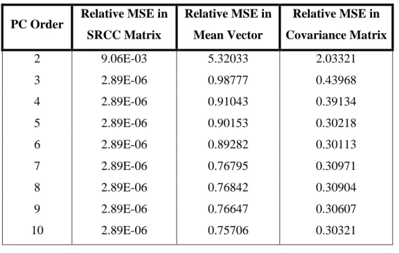
The PC coefficients of all 𝒙𝒊 can be evaluated from (5) and (6), and together with the samples of 𝝃, provide a set 𝑿(𝑷𝑪) containing 100,000 samples. The series has been truncated at a PC order of 8, as the representation manages to capture the features of the stochastic corrosion process with sufficient accuracy, for which the convergence plots have been presented ahead. From 𝑿(𝑷𝑪), samples of 𝑽(𝑷𝑪) can be obtained, along with the PC coefficients of each 𝒗𝒊, by using the transformation equation (9) above. Experimental observations of 𝑽 and 𝑿 have been contrasted against simulated PC samples, and the summary of all relevant comparisons has been presented in Table 1 for 𝑿 and Table 2 for 𝑽, in terms of the relative mean square error (MSE).
16 PC Order Relative MSE in
SRCC Matrix Relative MSE in Mean Vector Relative MSE in Covariance Matrix 2 9.06E-03 5.32033 2.03321 3 2.89E-06 0.98777 0.43968 4 2.89E-06 0.91043 0.39134 5 2.89E-06 0.90153 0.30218 6 2.89E-06 0.89282 0.30113 7 2.89E-06 0.76795 0.30971 8 2.89E-06 0.76842 0.30904 9 2.89E-06 0.76647 0.30607 10 2.89E-06 0.75706 0.30321
Table 1. Comparison of relevant statistics between experimental and PC samples of random vector 𝑿.
PC Order Relative MSE in SRCC Matrix Relative MSE in Mean Vector Relative MSE in Covariance Matrix 2 9.06E-03 0.07384 3.16995 3 2.89E-06 0.01137 0.51952 4 2.89E-06 0.01142 0.49408 5 2.89E-06 0.01061 0.47864 6 2.89E-06 0.01039 0.46482 7 2.89E-06 0.00911 0.46862 8 2.89E-06 0.00914 0.47148 9 2.89E-06 0.00901 0.47008 10 2.89E-06 0.00902 0.46408
17
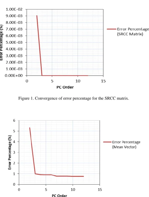
The tables show a convergence in all statistical errors beyond a PC order of 7. For visual purposes, the convergence plots for each of the errors have been presented in figures 1, 2 and 3. In each case, the error percentage of each statistic has been plotted against the PC order.
Figure 1. Convergence of error percentage for the SRCC matrix.
18
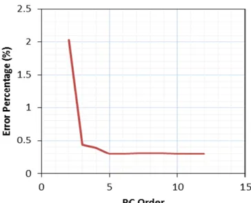
Figure 3. Convergence of error percentage for the covariance matrix.
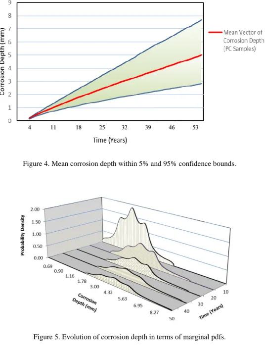
The simulated PC samples of corrosion depth have been represented in figure 4. The plot shows the mean vector of the corrosion depth 𝑽(𝑷𝑪), formed through PC expansion, within a lower and upper confidence bound of 5% and 95% respectively. Since the time period over which the pipeline is assessed has been taken as 50 years, and given a corrosion initiation time 𝒕𝟎 of 2.88 years, the experimental data has been taken from the 4th year to the 53rd year, hence giving us 50 years of corrosion depth data. Furthermore, an evolution of corrosion depth over those 50 years has been presented in terms of its marginal probability density, in figure 5.
19
Figure 4. Mean corrosion depth within 5% and 95% confidence bounds.
Figure 5. Evolution of corrosion depth in terms of marginal pdfs.
In addition, a plot showing the comparison between the mean vector of available corrosion depth measurements 𝑽, and the mean of the simulated depth 𝑽(𝑷𝑪) has been presented, in figure 6, to portray the accuracy of the PC representation in representing the stochastic corrosion process. For a PC order of 8, the error percentage between mean
20
vectors of the actual data and PC samples is about 0.009%, as is evident from the plot, where both vectors virtually overlap.
Figure 6. Mean vectors of corrosion depth for available measurements and PC samples against time.
Obtaining a PC representation of the stochastic process (i.e. pitting corrosion) is computationally inexpensive. Simulating PC samples mainly depends on the dimension of the available measurements, and here, generating a 100,000 x 50 matrix from the given dataset (100 x 50 measurements of corrosion depth), can be done in rather quickly. It is to be noted however, that depending on the technique used to modify the non-positive definite matrix, the time taken to simulate PC samples may increase considerably.
Once the PC coefficients have been obtained for specified points of time 𝒕 at which the measurements are available, the corrosion depth at any time 𝑻∉ 𝐭 can be generated by interpolating the PC coefficients at that given time 𝑻, from which the corresponding sample of corrosion depth can be obtained. The technique for interpolation depends on the
21
trend followed by the data, and should be chosen accordingly for a given stochastic process.
3.3. Prediction of Corrosion Growth
Once the PC representation of corrosion depth propagation over a given period of time has been obtained, the depth at any other point of time can be obtained by interpolation, as discussed above. In this study, as a method of validation, once the PC samples 𝑽(𝑷𝑪) have been obtained, the PC coefficients for the first 25 years of corrosion data have been used to extrapolate the coefficients for the next 25 years. Once the extrapolated coefficients have been approximated, the corrosion depth samples, 𝑽𝒑𝒓𝒆𝒅(𝑷𝑪), for those 25 years in the future can be constructed. Once the predicted depth has been obtained, it can be compared to the PC samples already available for those 25 years. A simple linear interpolation technique has been used in this research, which is able to accurately predict corrosion growth. The accuracy of prediction was measured by taking the relative MSE between the available PC samples for the remaining 25 years, and the predicted PC samples for that time period, which turned out to be 0.0982%. Figure 7 shows the mean predicted corrosion depth 𝑽𝒑𝒓𝒆𝒅(𝑷𝑪) against the mean simulated corrosion depth 𝑽(𝑷𝑪).
22
Figure 7. Comparison between mean vectors of simulated and predicted corrosion depth.
Again, it is crucial to identify the behavior of the stochastic process, and accordingly, adopt a suitable method to obtain the coefficients. In this study, the corrosion depth increases at an exponential rate initially, but eventually becomes more linear over time. A linear or cubic extrapolation process can provide sufficient prediction accuracy for such data. However, for a random process that might heavily fluctuate with time, other regression methods can be utilized instead.
23
4. RELIABILITY-BASED LIFE CYCLE COST MANAGEMENT
Assessment of reliability has been carried out in a way similar to Zhou’s work [28]. As mentioned earlier, only a section of the pipeline is being analyzed, which is assumed to contain the pitting corrosion hotspot. Failure has been assumed to be dependent on this corrosion pit’s crack depth propagation. The reliability framework for buried pipelines which incorporates the PC expansion has been described ahead in detail.
4.1. Limit State Functions
Two limit state functions (LSFs) have been used to define pipeline failure events, namely small leak, and burst. When a defect, which refers to the corrosion pit, penetrates the pipeline wall to 80% of its thickness, the failure scenario is defined as a small leak 𝒈𝒔(𝒕), represented by the following equation,
𝒈𝒔(𝒕) = 𝟎. 𝟖 ∙ 𝒘 − 𝒅𝒎𝒂𝒙(𝒕) (10) Here, 𝒘 represents the wall thickness of the pipe, and 𝒅𝒎𝒂𝒙(𝒕) is the maximum corrosion depth at time 𝒕. This equation is consistent with industrial practice, where a small leak is considered to occur when the maximum defect depth is 80% of the wall thickness, as opposed to its entire thickness 𝒘.
Due to the internal pressure, when the pipe wall undergoes plastic collapse at the defect location prior to the penetration of the pipe wall, a burst failure is considered to occur. The limit state function for burst 𝒈𝒃(𝒕) is given by,
24
In this equation, 𝐫𝐛(𝐭) is the resisting burst pressure, and 𝐩 is the pipe’s internal pressure. To evaluate 𝐫𝐛(𝐭), two models have been used – the PCORRC model [48] given by equation (12), and the DNV RP-F101 [49] given by equation (13). Their relationship with resisting pressure can be defined as follows,
𝒓𝒃(𝒕) = 𝝌𝒎∙𝟐∙𝝈𝒖∙𝒘 𝑫 . [𝟏 − 𝒅𝒎𝒂𝒙(𝒕) 𝒘 (𝟏 − 𝒆𝒙𝒑 (− 𝟎.𝟏𝟓𝟕∙𝑳(𝒕) √𝟎.𝟓∙𝑫(𝒘−𝒅𝒎𝒂𝒙(𝒕))))] (12) 𝒓𝒃(𝒕) =𝟐.𝑺𝑴𝑻𝑺.𝒘𝑫 . [𝟏− 𝒅𝒎𝒂𝒙(𝒕) 𝒘 𝟏− 𝒅𝒎𝒂𝒙(𝒕) 𝒘 𝑴 ], where 𝑴 = √1 + 0.31 ∙ (𝐿(𝑡) √𝐷∙𝑤) 2 (13)
Where 𝝌𝐦 is a multiplicative model error factor, used in this particular model, 𝛔𝐮 is the ultimate tensile strength of the pipe material, 𝐃 is the pipe diameter and 𝐋(𝐭) is the length of the corrosion defect. For DNV RP-F101, SMTS represents the specified minimum tensile strength and M is the bulging factor. In this case, 𝛔𝐮 and SMTS are the same. The value of each of these parameters has been taken from literature [28]. While other models area available, PCORRC and DNV RP-F101 have been used and compared because they are similar, reasonably accurate, and only require the corrosion pit length and maximum depth as defect based geometrical input. The results for each of them have been presented ahead in this document.
Currently, as no experimental data exists for defect length 𝐋(𝐭), the linear model used by Zhou and Nessim [28] has been utilized, in which the defect length has grown at a constant rate with an initial mean value of 30 mm, but the rate itself has a lognormal distribution, with a mean of 1.0 mm/year and standard deviation of 0.5 mm/year. Hence,
25
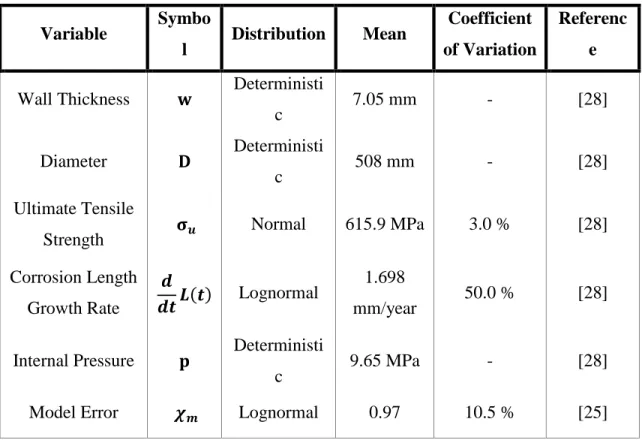
in a time period of 50 years, the average defect length is equal to 80.0 mm. At any point prior to the initiation time 𝐭𝟎, the defect length has been considered zero, and its growth parameters have been accordingly modified to attain the same average value, as obtained in the original linear model. Each of these random variables has been summarized in table 3, shown below. Variable Symbo l Distribution Mean Coefficient of Variation Referenc e Wall Thickness 𝐰 Deterministi
c 7.05 mm - [28]
Diameter 𝐃 Deterministi
c 508 mm - [28]
Ultimate Tensile
Strength 𝛔𝒖 Normal 615.9 MPa 3.0 % [28]
Corrosion Length Growth Rate 𝒅 𝒅𝒕𝑳(𝒕) Lognormal 1.698 mm/year 50.0 % [28]
Internal Pressure 𝐩 Deterministi
c 9.65 MPa - [28]
Model Error 𝝌𝒎 Lognormal 0.97 10.5 % [25]
Table 3. Random variables and parameters associated with the pipeline.
4.2. Optimization Methodology
Since the optimum repair schedule is dependent on expected values of costs and failures, the concept of predictive maintenance has been employed. All-inclusive costs of inspection, repair and failure have been revised to match their values at the time of
26
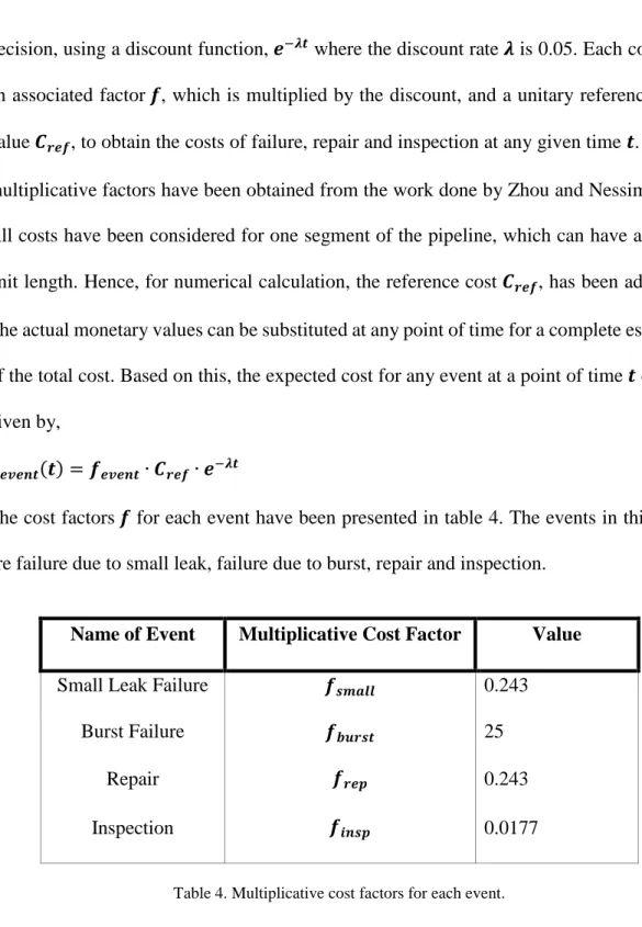
decision, using a discount function, 𝒆−𝝀𝒕 where the discount rate 𝝀 is 0.05. Each cost has an associated factor 𝒇, which is multiplied by the discount, and a unitary reference cost value 𝑪𝒓𝒆𝒇, to obtain the costs of failure, repair and inspection at any given time 𝒕. These multiplicative factors have been obtained from the work done by Zhou and Nessim [28]. All costs have been considered for one segment of the pipeline, which can have a given unit length. Hence, for numerical calculation, the reference cost 𝑪𝒓𝒆𝒇, has been adopted. The actual monetary values can be substituted at any point of time for a complete estimate of the total cost. Based on this, the expected cost for any event at a point of time 𝒕 can be given by,
𝑪𝒆𝒗𝒆𝒏𝒕(𝒕) = 𝒇𝒆𝒗𝒆𝒏𝒕∙ 𝑪𝒓𝒆𝒇∙ 𝒆−𝝀𝒕 (14) The cost factors 𝒇 for each event have been presented in table 4. The events in this case are failure due to small leak, failure due to burst, repair and inspection.
Name of Event Multiplicative Cost Factor Value
Small Leak Failure 𝒇𝒔𝒎𝒂𝒍𝒍 0.243
Burst Failure 𝒇𝒃𝒖𝒓𝒔𝒕 25
Repair 𝒇𝒓𝒆𝒑 0.243
Inspection 𝒇𝒊𝒏𝒔𝒑 0.0177
Table 4. Multiplicative cost factors for each event.
The cost of a small leak is based on excavating and repairing the pipeline at the corrosion pit location. Burst failure cost includes excavating and replacing the pipe
27
segment while also incorporating financial compensation for deaths and damage to property. The value of 25 has been assigned to the damage done to one property, without any casualties. In this paper, one defect per unit length of the pipeline has been assumed, which is significant enough to dominate failure. Studies exist, which have concentrated on both, single and multiple defects [25, 28, 29, 30]. Additionally, further work can look into the use of system reliability to address multiple correlated corrosion defects, and their combined effect on pipeline failure. However, in this case, the maintenance strategy has focused on analyzing a single yet significant defect, for one segment of the pipeline.
In order to come up with a maintenance schedule, deciding the time of each inspection, and consequently repair, is paramount. Based on this, the two design variables that have been considered in this study are, the time to first inspection 𝒕𝒊𝒏𝒔𝒑𝟏, and the interval between each successive inspection 𝜹𝒕𝒊𝒏𝒔𝒑. The time to first inspection and consequent inspection intervals have been considered as separate design variables, as 𝒕𝒊𝒏𝒔𝒑𝟏 indicates the necessity of subsequent inspections, and how often they need to be scheduled. Other important factors would be the material and geometric parameters such as pipeline diameter, internal pressure, tensile strength and wall thickness. However, as important as they are in the safety of pipelines, the values of variables such as wall thickness are bound by design codes and guidelines, while diameter and pressure depend on operation requirements. Hence, this research has focused on developing an effective maintenance strategy, based on different times of inspection.
28
The main difference between the expected costs of inspection and other events is that the number of inspections can be found out ahead of time, based on the time interval between each inspection. Hence, the inspections are already considered to be paid for. The number of failures and repairs are unknown beforehand, and can only be found by inspecting the pipeline at those points of time. By incorporating the probability of failure or repair, obtained by Monte Carlo sampling, and multiplying it with the respective cost factors and discount function, the cost of each event can be calculated.
If the design life of the pipeline is represented by 𝑳𝑻, given the time to first inspection, and the intervals between subsequent inspections, we can calculate the number of inspections as follows,
𝑵𝒊𝒏𝒔𝒑 = 𝟏 + 𝒇𝒍𝒐𝒐𝒓 (𝑳𝑻−𝒕𝒊𝒏𝒔𝒑𝟏
𝜹𝒕𝒊𝒏𝒔𝒑 ) (15)
Here, the 𝒇𝒍𝒐𝒐𝒓 function returns the largest integer that is less than or equal to its argument. Based on all the available variables, the objective function, where the total expected cost 𝑬(𝑪𝑻), has to be minimized, can be represented as,
𝑬(𝑪𝑻) = 𝑪𝒓𝒆𝒇+ 𝑵𝒊𝒏𝒔𝒑∙ 𝑪𝒊𝒏𝒔𝒑+ 𝑬(𝑪𝒓𝒆𝒑) + 𝑬(𝑪𝒇𝒂𝒊𝒍) (16) The expected costs can further be given by,
𝑬(𝑪𝒇𝒂𝒊𝒍) = 𝑪𝒔𝒎𝒂𝒍𝒍×𝑷𝒔𝒎𝒂𝒍𝒍+ 𝑪𝒃𝒖𝒓𝒔𝒕×𝑷𝒃𝒖𝒓𝒔𝒕
𝑬(𝑪𝒓𝒆𝒑) = 𝑪𝒓𝒆𝒑×𝑷𝒏𝒐𝒇𝒂𝒊𝒍 (17) In the equation, 𝑷𝒏𝒐 𝒇𝒂𝒊𝒍, 𝑷𝒔𝒎𝒂𝒍𝒍 and 𝑷𝒃𝒖𝒓𝒔𝒕 represent the probability of repair, small leak and failure. In addition, another constraint on the probability of failure has been imposed, to ensure that the total combined probability of failure 𝑷𝒄𝒐𝒎𝒃, never exceeds its maximum
29
allowable limit 𝑷𝒍𝒊𝒎𝒊𝒕. The combined probability of failure can be interpreted in terms of either the overall maximum probability of failure or the average probability of failure, both during the lifetime. If this defined failure probability does go beyond the threshold at any point of time, the maximum time between successive inspections is adjusted to satisfy this condition. This has been discussed in sections of the paper ahead, in more detail. For clarity, the relationship for the combined probability of failure has been given below, 𝑷𝒄𝒐𝒎𝒃 = (𝑷𝒔𝒎𝒂𝒍𝒍∪ 𝑷𝒃𝒖𝒓𝒔𝒕)
= 𝑷𝒔𝒎𝒂𝒍𝒍+ 𝑷𝒃𝒖𝒓𝒔𝒕− (𝑷𝒔𝒎𝒂𝒍𝒍∩ 𝑷𝒃𝒖𝒓𝒔𝒕) (18) The probability of repair 𝑷𝒏𝒐 𝒇𝒂𝒊𝒍, represents all the samples that have neither failed to due to small leak or burst, thus can be re-written as,
𝑷𝒏𝒐 𝒇𝒂𝒊𝒍= 𝟏 − 𝑷𝒄𝒐𝒎𝒃 (19) The event of repair is considered to be ‘no failure’, as in any case, at the time of inspection, either the failure event is identified as a leak or burst, and its corresponding cost applied, or if no failure occurs, the pipeline is just repaired and restarted, and the repair cost is taken instead.
In order to solve the optimization problem, the expected cost 𝑬(𝑪𝑻) needs to be minimized by finding feasible values for 𝒕𝒊𝒏𝒔𝒑𝟏 and 𝜹𝒕𝒊𝒏𝒔𝒑, subject to the following constraints,
𝒕𝒊𝒏𝒔𝒑𝟏𝝐(𝒕𝒊𝒏𝒔𝒑𝟏𝒎𝒊𝒏 , 𝒕𝒊𝒏𝒔𝒑𝟏𝒎𝒂𝒙 ),
𝜹𝒕𝒊𝒏𝒔𝒑𝝐(𝜹𝒕𝒊𝒏𝒔𝒑𝒎𝒊𝒏, 𝜹𝒕𝒊𝒏𝒔𝒑𝒎𝒂𝒙)
30
Where 𝒕𝒊𝒏𝒔𝒑𝟏𝒎𝒊𝒏 and 𝒕𝒊𝒏𝒔𝒑𝟏𝒎𝒂𝒙 are the lower and upper bounds respectively, of the time to first inspection, taken as (5.0, 30.0) for this study. Similarly, 𝜹𝒕𝒊𝒏𝒔𝒑𝒎𝒊𝒏 and 𝜹𝒕𝒊𝒏𝒔𝒑𝒎𝒂𝒙 are the lower and upper bounds of the inspection intervals, taken as (5.0, 30.0) for this study.
4.3. Implementation of the Maintenance Strategy
The expected number of failures and repairs are calculated at the given time of inspection by using the Monte Carlo method. At the inspection time 𝒕, each sample of corrosion depth 𝒅𝒎𝒂𝒙(𝒕), as well as the samples generated for the resisting pressure 𝒓𝒃(𝒕), is checked against their limit state functions. If the value of LSF for either small leak or burst is zero or negative, then the respective failure event is considered to have taken place. In case both failures occur at a given time simultaneously, burst is given precedence over small leak, as its cost and consequences are higher, and a replacement of the pipeline section due to burst also covers the renewal condition for small leak. The remaining samples, where no failure whatsoever has occurred, are still corroded to an extent. Hence these samples require the pipeline to be repaired instead, and the corresponding cost factor for repair or ‘no fail’ is applied.
It must be made clear that, after an inspection, a complete restart will always occur due to either repair or failure. Hence, at the time following the inspection, the corrosion growth, burst pressure and defect length are restarted based on a new generated corrosion pit. The material properties of the pipeline are also resampled. Also, the solution is taken to be viable only if 𝑷𝒄𝒐𝒎𝒃 is within the threshold. In other words, the total expected cost 𝑬(𝑪𝑻), obtained for a set of 𝒕𝒊𝒏𝒔𝒑𝟏 and 𝜹𝒕𝒊𝒏𝒔𝒑, has been considered only when the
31
combined probability of failure does not exceed the permissible limit. Since the pipeline needs to be kept in service continuously, once the restart occurs, the simulation carries on till the end of the pipeline’s lifetime.
4.4. Evolution of Probability of Failure
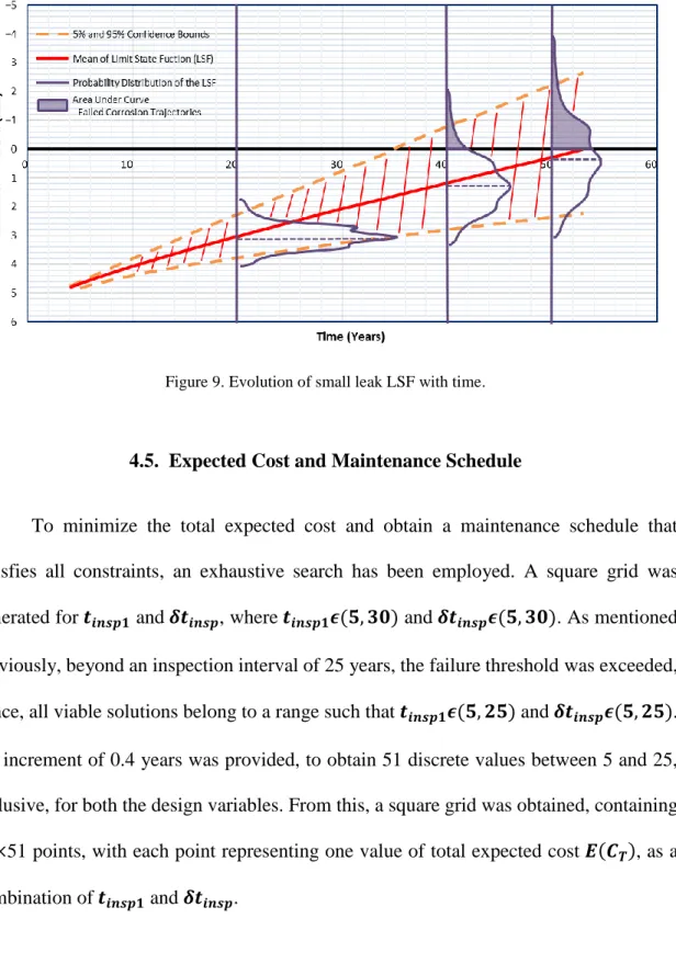
The combined probability of pipeline failure has been used as a criterion to decide the feasibility of any value of the total expected cost. It corresponds to the level of risk that is acceptable while operating and maintaining the pipeline. The overall threshold for the maximum probability of failure in this study has been considered as 5% or 0.05. Hence, 𝑷𝒄𝒐𝒎𝒃 cannot exceed this limit at any point of time. The evolution of combined probability of failure with time, when no maintenance strategy has been implemented, has been presented in figure 8. Based on this threshold, the individual evolution of the LSF for small leak with time has been shown in figure 9. The marginal distributions at the 17th, 37th and 47th year of the time period of 53 years have been plotted, to show the extent of failure over time. Most of the failures due to small leak primarily take place after the 30th year for which the data has been generated.
32
Figure 8. Evolution of maximum probability of failure with time.
Based on the pipeline attributes, failures due to burst often occurred prior to small leak in this study. Hence, in most cases, the predominant factor affecting the cost of failure, and consequently, the total expected cost, has been the burst LSF. Figure 8 shows that the combined probability of failure exceeds the threshold by the 28th year, i.e. at the 25th year
since the corrosion data of the pipeline is available. Hence, the maximum inspection interval for a viable solution is 25 years. This means that once pitting corrosion starts, it breaches the acceptable risk level in 25 years. The time to first inspection 𝒕𝒊𝒏𝒔𝒑𝟏, and the inspections intervals 𝜹𝒕𝒊𝒏𝒔𝒑, both have their upper limit restricted to 25 years, beyond which viable solutions constrained by this threshold cannot be obtained.
33
Figure 9. Evolution of small leak LSF with time.
4.5. Expected Cost and Maintenance Schedule
To minimize the total expected cost and obtain a maintenance schedule that satisfies all constraints, an exhaustive search has been employed. A square grid was generated for 𝒕𝒊𝒏𝒔𝒑𝟏 and 𝜹𝒕𝒊𝒏𝒔𝒑, where 𝒕𝒊𝒏𝒔𝒑𝟏𝝐(𝟓, 𝟑𝟎) and 𝜹𝒕𝒊𝒏𝒔𝒑𝝐(𝟓, 𝟑𝟎). As mentioned previously, beyond an inspection interval of 25 years, the failure threshold was exceeded, hence, all viable solutions belong to a range such that 𝒕𝒊𝒏𝒔𝒑𝟏𝝐(𝟓, 𝟐𝟓) and 𝜹𝒕𝒊𝒏𝒔𝒑𝝐(𝟓, 𝟐𝟓). An increment of 0.4 years was provided, to obtain 51 discrete values between 5 and 25, inclusive, for both the design variables. From this, a square grid was obtained, containing 51×51 points, with each point representing one value of total expected cost 𝑬(𝑪𝑻), as a combination of 𝒕𝒊𝒏𝒔𝒑𝟏 and 𝜹𝒕𝒊𝒏𝒔𝒑.
34
Based on the exhaustive search, the minimum cost was obtained for 𝒕𝒊𝒏𝒔𝒑𝟏 = 19 years, and 𝜹𝒕𝒊𝒏𝒔𝒑 = 18.6 years, both from the time the corrosion data is available (4th year of 53 years). The plot for 𝑬(𝑪𝑻) has been represented by figure 10, where 𝒕𝒊𝒏𝒔𝒑𝟏 is constant at 19 years, and 𝜹𝒕𝒊𝒏𝒔𝒑 varies from 5 to 25 years.
Figure 10. Expected cost variation for 𝒕𝒊𝒏𝒔𝒑𝟏 = 19 years and the range of 𝜹𝒕𝒊𝒏𝒔𝒑.
The graph for 𝑬(𝑪𝑻) is quite discontinuous, and these points of discontinuity occur when the number of inspections changes. For examples, given that the first inspection is after 19 years, and having an interval 𝜹𝒕𝒊𝒏𝒔𝒑 = 15 years, yields a total of 3 inspections in 50 years. This holds for 𝜹𝒕𝒊𝒏𝒔𝒑 = 15.4 years as well. However, at 𝜹𝒕𝒊𝒏𝒔𝒑 = 15.8 years, the number of inspections changes from 3, to 2. Consequently, the expected cost takes a sharp drop, and this behavior is evident in figure 10. The convexity of the cost curve is due to the tradeoff between the cost of repair and failure, against the cost of several inspections.
(Years)
(𝑬
[𝑪𝑻
])
35
For a small 𝜹𝒕𝒊𝒏𝒔𝒑, there will be several inspections over the pipeline’s lifetime, resulting in a high cost of inspection, which dominates the total cost. On the other hand, very few inspections, or just one inspection, results in a high number of failures, especially burst failures, which influence the total expected cost. Within each valley (where 𝑵𝒊𝒏𝒔𝒑 is constant), the cost curve is smooth, and a local minimum for that particular 𝑵𝒊𝒏𝒔𝒑 can be evaluated. The entire grid for the total expected cost 𝑬(𝑪𝑻), has been presented in figure 11. The total cost for each combination of 𝒕𝒊𝒏𝒔𝒑𝟏 and 𝜹𝒕𝒊𝒏𝒔𝒑 has been shown in the grid, which has 51×51 points in total.
36
4.6. Comparison of Optimization Techniques
In addition to an exhaustive search, an inbuilt optimization function in MATLAB, based on genetic algorithm techniques, has been used as validation for the exhaustive search. The same code, applied to the exhaustive search, has been passed through a GA function. The results were found to be the same, for both 𝒕𝒊𝒏𝒔𝒑𝟏 and 𝜹𝒕𝒊𝒏𝒔𝒑. However, while the exhaustive search took about 15 hours to arrive at the optimum maintenance schedule, it was achieved in close to 8 hours by the GA technique, making it more computationally efficient.
4.7. Sensitivity Analysis for Burst Failure Costs
A sensitivity analysis with respect to different burst failure costs has also been carried out, to assess the variation of the objective function, i.e. total expected cost 𝑬(𝑪𝑻), based on different failure scenarios. The lowest cost of burst failure has a cost factor 𝒇𝒃𝒖𝒓𝒔𝒕 = 25, while the highest cost factor for burst is 𝒇𝒃𝒖𝒓𝒔𝒕 = 200. Along with these two values, 3 intermediate values for 𝒇𝒃𝒖𝒓𝒔𝒕 have been chosen, which are 50, 75 and 150. The results have been shown in figure 12, where for 𝒕𝒊𝒏𝒔𝒑𝟏= 19 years, the total expected costs have been plotted against the entire range of inspections intervals, (𝜹𝒕𝒊𝒏𝒔𝒑). It is evident, that as the cost of burst failure increases, the minimum total expected cost also increases.
37
Figure 12. Total expected costs for different cost factors 𝒇𝒃𝒖𝒓𝒔𝒕, at 𝒕𝒊𝒏𝒔𝒑𝟏= 19 years.
The values of minimum 𝑬(𝑪𝑻) for different burst failure factors 𝒇𝒃𝒖𝒓𝒔𝒕 have been summarized in table 5 below.
Value of 𝒇𝒃𝒖𝒓𝒔𝒕 Minimum 𝑬(𝑪𝑻) 25 1.141872 50 1.1613 75 1.182 150 1.2269 200 1.2741
Table 5. Minimum 𝑬(𝑪𝑻) values for different burst failure factors 𝒇𝒃𝒖𝒓𝒔𝒕.
(𝑬
[𝑪
𝑻
])
38
4.8. Comparison between Different Pressure Models
The results for the maintenance schedule have been presented for DNV RP-F101, in terms of the design variables and minimum cost. The optimum values for this model were very similar to PCORRC, with minor differences. Based on the exhaustive search, the time to first inspection 𝒕𝒊𝒏𝒔𝒑𝟏 was found to be 18.6 years, and the interval of subsequent inspections 𝜹𝒕𝒊𝒏𝒔𝒑 was 17.4 years. The failure threshold, for a maximum probability of failure as 5%, was exceeded in the same time of 25 years between any two inspections. The minimum cost for this particular maintenance schedule was 1.1406. Table 6 below compares the results of the two pressure models.
Parameter
Burst Pressure Models
PCORRC DNV RP-F101
Minimum 𝑬(𝑪𝑻) 1.142 1.1406
Optimum 𝒕𝒊𝒏𝒔𝒑𝟏 19 18.6
Optimum 𝜹𝒕𝒊𝒏𝒔𝒑 18.6 17.4
Table 6. Comparison of different burst pressure models.
In this case, GA was used to find the optimum maintenance strategy as well, and the results were in agreement with the exhaustive search for both the design variables and the minimum cost. The plot for 𝑬(𝑪𝑻), for DNV RP-F101 has been represented by figure
39
13, where 𝒕𝒊𝒏𝒔𝒑𝟏 is constant at 18.6 years, and 𝜹𝒕𝒊𝒏𝒔𝒑 varies from 5 to 25 years. The entire grid for the total expected cost 𝑬(𝑪𝑻), has also been presented, in figure 14.
Figure 13. Expected cost variation for 𝒕𝒊𝒏𝒔𝒑𝟏 = 18.6 years and the range of 𝜹𝒕𝒊𝒏𝒔𝒑.
Figure 14. Expected cost grid for different 𝒕𝒊𝒏𝒔𝒑𝟏 and 𝜹𝒕𝒊𝒏𝒔𝒑, for DNV RP-F101. Min 𝑬(𝑪𝑻) = 1.1406 (Years) (𝑬 [𝑪 𝑻 ])
40
5. CONCLUSIONS
In this research, the lifecycle management of pipelines subjected to external pitting corrosion was addressed, within the context of reliability assessment. This was done via probabilistic optimization, where the total cost associated with operating and maintaining buried pipelines was minimized, while developing an effective maintenance strategy. These lifecycle costs included the costs of inspection, repair and failure, which were converted to their respective values at the decision time, using a discount function. The maintenance schedule was obtained by optimizing two variables, which were the time to first inspection and the time between successive inspections. In addition, a constraint on the allowable probability of failure was imposed, which in turn provided effective maintenance strategies for different risk levels. Based on this, the model is also capable of producing a maintenance schedule, for a given maximum cost, while presenting the maximum and average probabilities of failure for each combination of the design variables.
The model used to represent the process of corrosion, was based on polynomial chaos, which avoids the conservatism in previous models by assuming the corrosion pit depth as a random variable. It was shown to have a high degree of accuracy, and sufficiently captured the stochastic features of an experimentally observed external pitting corrosion process, assumed to be second order, as well as Gaussian and non-stationary. The technique involves estimating the joint probability distribution of measured data, which is completely characterized by a set of marginals and a correlation
41
matrix, approximated from experimental samples, and constructing a PC representation such that its associated joint PDF is within a desired tolerance to the distribution obtained from the measurements. The correlation function, which is the SRCC matrix, enforces the statistical dependency between components of 𝝃𝒌. Consequently, the PC representation so constructed can be readily utilized within the framework to propagate the uncertainty associated with the corrosion process.
The optimization results for the maintenance schedule were obtained using an exhaustive search, and verified by using an inbuilt genetic algorithm function. While the outcome in terms of inspection times remained the same, the optimization function was evaluated in a shorter time span by GA techniques, when compared to the exhaustive search.
Given the results, the reliability framework employed during this research for corroding pipelines can also be applied to other deteriorating structural systems in a broader sense, and accurately capture the uncertainties associated them. However, in reality, this accuracy would be dependent on identifying the actual sources of uncertainty, and how they can be represented within the system as parameters. Future work could focus on incorporating system reliability and addressing the combined failure due to multiple hotspots, using this technique, for pipeline integrity management programs.
42 REFERENCES
[1] Aktan, A. E., Farhey, D. N., Brown, D. L., Dalal, V., Helmicki, A. J., Hunt, V. J., & Shelley, S. J. (1996). Condition assessment for bridge management. Journal of Infrastructure Systems, 2(3), 108-117.
[2] Ahammed, M. (1997). Prediction of remaining strength of corroded pressurised pipelines. International Journal of Pressure Vessels and Piping, 71(3), 213-217. [3] Tao, Z., Corotis, R. B., & Ellis, J. H. (1994). Reliability-based bridge design and life
cycle management with Markov decision processes. Structural Safety, 16(1-2), 111-132.
[4] Orcesi, A. D., Frangopol, D. M., & Kim, S. (2010). Optimization of bridge maintenance strategies based on multiple limit states and monitoring. Engineering Structures, 32(3), 627-640.
[5] Orcesi, A. D., & Frangopol, D. M. (2011). Optimization of bridge maintenance strategies based on structural health monitoring information. Structural Safety,
33(1), 26-41.
[6] Estes, A. C., & Frangopol, D. M. (2001). Minimum expected cost-oriented optimal maintenance planning for deteriorating structures: Application to concrete bridge decks. Reliability Engineering & System Safety, 73(3), 281-291.
43
[7] Chassiakos, A. P., Vagiotas, P., & Theodorakopoulos, D. D. (2005). A knowledge-based system for maintenance planning of highway concrete bridges. Advances in Engineering Software, 36(11), 740-749.
[8] Straub, D., & Faber, M. H. (2005). Risk based inspection planning for structural systems. Structural Safety, 27(4), 335-355.
[9] Streicher, H., Joanni, A., & Rackwitz, R. (2008). Cost-benefit optimization and risk acceptability for existing, aging but maintained structures. Structural Safety, 30(5), 375-393.
[10] Okasha, N. M., & Frangopol, D. M. (2009). Lifetime-oriented multi-objective optimization of structural maintenance considering system reliability, redundancy and life-cycle cost using GA. Structural Safety, 31(6), 460-474.
[11] Sanchez-Silva, M., Klutke, G. A., & Rosowsky, D. V. (2011). Life-cycle performance of structures subject to multiple deterioration mechanisms. Structural Safety, 33(3), 206-217.
[12] Cremona, C. (1996). Reliability updating of welded joints damaged by fatigue. International Journal of Fatigue, 18(8), 567-575.
[13] Kulkarni, S. S., & Achenbach, J. D. (2007). Optimization of inspection schedule for a surface-breaking crack subject to fatigue loading. Probabilistic Engineering
44
[14] Valdebenito, M. A., & Schuëller, G. I. (2010). Design of maintenance schedules for fatigue-prone metallic components using reliability-based optimization. Computer Methods in Applied Mechanics and Engineering, 199(33), 2305-2318.
[15] Riahi, H., Bressolette, P., Chateauneuf, A., Bouraoui, C., & Fathallah, R. (2011). Reliability analysis and inspection updating by stochastic response surface of fatigue cracks in mixed mode. Engineering Structures, 33(12), 3392-3401.
[16] Biondini, F., & Frangopol, D. M. (2009). Lifetime reliability-based optimization of reinforced concrete cross-sections under corrosion. Structural Safety, 31(6), 483-489.
[17] Bastidas-Arteaga, E., & Schoefs, F. (2012). Stochastic improvement of inspection and maintenance of corroding reinforced concrete structures placed in unsaturated environments. Engineering Structures, 41, 50-62.
[18] Caleyo, F., Velázquez, J. C., Valor, A., & Hallen, J. M. (2009). Probability distribution of pitting corrosion depth and rate in underground pipelines: A Monte Carlo study. Corrosion Science, 51(9), 1925-1934.
[19] Velázquez, J. C., Caleyo, F., Valor, A., & Hallen, J. M. (2009). Predictive model for pitting corrosion in buried oil and gas pipelines. Corrosion, 65(5), 332-342.
[20] Velázquez, J. C., Caleyo, F., Valor, A., & Hallen, J. M. (2010). Technical Note: Field study—Pitting corrosion of underground pipelines related to local soil and pipe characteristics. Corrosion, 66(1), 016001-016001.