Document downloaded from:
This paper must be cited as:
The final publication is available at
http://dx.doi.org/10.1016/j.asoc.2010.10.004 http://hdl.handle.net/10251/50488
Lughofer, E.; Macian Martinez, V.; Guardiola García, C.; Klement, EP. (2011). Identifying static and dynamic prediction models for NOx emissions with evolving fuzzy systems. Applied Soft Computing. 11(2):2487-2500. doi:10.1016/j.asoc.2010.10.004.
Identifying Static and Dynamic Prediction
Models for NOx Emissions with Evolving
Fuzzy Systems
Edwin Lughofer*
aVicente Maci´
an
bCarlos Guardiola
bErich Peter Klement
aaDepartment of Knowledge-based Mathematical Systems/Fuzzy Logic Laboratorium
Linz-Hagenberg, Johannes Kepler University of Linz, Austria
bCMT-Motores T´ermicos/Universidad Polit´ecnica de Valencia, Spain
Abstract
Antipollution legislation in automotive internal combustion engines requires active control of pollutant formation and emissions. In addition to new technologies, like selective catalyst systems or diesel particulate filters, predictive emission models are needed. These models are of great use in the system calibration phase, and also can be integrated for the engine control and on-board diagnosis tasks. In this pa-per, fuzzy modelling of the NOx emissions of a diesel engine is investigated, which overcomes some drawbacks of pure engine mapping or analytical physical-oriented models. For building up the fuzzy NOx prediction models, theFLEXFIS approach (short for FLEXible Fuzzy Inference Systems) is applied, which automatically ex-tracts an appropriate number of rules and fuzzy sets by an evolving version of vec-tor quantization (eVQ) and estimates the consequent parameters of Takagi-Sugeno fuzzy systems with the local learning approach in order to optimize the least squares functional. The predictive power of the fuzzy NOx prediction models is compared with that one achieved by physical-oriented models based on high-dimensional en-gine data recorded during steady-state and dynamic enen-gine states.
Key words: Combustion engines, NOx emissions, analytical physical-oriented models, Takagi-Sugeno fuzzy systems, FLEXFIS, high-dimensional data, steady-state and dynamic engine states
1 Introduction and Motivation
Automotive antipollution legislation are increasingly stringent, which boost technology innovations for the control of engine emissions. A combination of active methods (which directly address the pollutant formation mechanism) and passive methods (which avoid the pollutant emission) is needed. Between the first, innovations in fuel injection and combustion systems, and also ex-haust gas recirculation [1], have been successfully applied to spark ignited and compressed ignited engines.
Passive methods include three-way catalytic converters, oxidation catalytic converters, diesel particulate filters, NOx (nitrogen oxides) adsorbers or se-lective reduction catalyst [2]. Several of these technologies need the pollutant production to be known in order to control the addition of different additives needed for the system operation or regeneration.
In this frame, pollutant emission models (in particular NOx models) are cur-rently under development to be included in the engine control system and the on-board diagnostic system. This action is necessary particularly to optimise the control of NOx after-treatment devices as NOx traps and selective reduc-tion catalyst. NOx is one of the more important pollutants in compression ig-nited engines. NOx formation is mostly due to the oxidation of the atmospheric nitrogen during the combustion process at high local temperatures, which is explained through the well known extended Zeldovich formation mechanism [3] (although some additional mechanisms can occur [4]).
There are several ways for estimating the amount of a given pollutant that reaches the after-treatment device [5]:
• A direct mapping of the pollutant emitted by a reference engine as a function of rotation speed and torque can be used. This method, usually implemented as a series of look-up tables, is straightforward because it has exactly the same structure of many other maps already available in the ECU, and hence calibration engineers can easily calibrate them.
• A physical-based model developed by engine experts (based on the knowl-edge of the inner physics), based on some engine operating parameters con-tinuously registered by the ECU can be used.
• A direct measurement of the pollutant emission in the exhaust gases can be performed.
Although the latter option is ideal because is the only that fully addresses the diagnosis function, the technology in order to be able to produce low cost, precise and drift-free sensors, however, is still under development depending on the considered pollutant [6]. Hence, emission models are of great interest, leaving the first two options.
Direct engine maps are usually unable to compensate for production variations and variations in the operating conditions (e.g., warming-up of the engine, altitude, external temperature, etc.) in the engine along the vehicle lifetime. Hence, they are usually not flexible enough to predict the NOx content with sufficient accuracy. Furthermore, important human intervention is needed for fixing the structure and the input variables of the model, which is usually time-intensive as model calibration is complex and difficult to automate. Physical-based models compensate this weakness of direct engine maps by including a deeper knowledge of experts about the emission behaviour of an engine. However, this direct physical approach based on the complete tracking of the NO formation kinetics is usually discarded for the online application because of the huge computational power required and because excellent de-scription of the flame instantaneous local conditions is needed. Furthermore, the deduction of physical-based models often require significant development time and is usually very specific (applicable only for one concrete engine). Reviews and different model implementations can be found in the literature [7–9].
1.1 Our Fuzzy Modelling Approach
Our modelling approach tries to find a compromise between a physical-oriented and a pure mapping approach (the latter usually only applicable in lower dimensional spaces) by extracting automatically high-dimensional non-linear fuzzy models from static as well as dynamic measurements recorded during the test phases of an engine. These measurements reflect the emission be-havior of the corresponding engine and hence provide a representation of the intrinsic relations between some physical measurement channels (such as tem-peratures, pressures, engine speed, torque etc.) and the NOx concentration in the exhaust gases in the emission. Our methodology of a machine-learning driven building up of fuzzy models is able to recognize this relation and hence to map input values (from a subset of measurement channels) onto the NOx concentration (used as target) appropriately, fully automatically and with high precision. The learning algorithm consists of two phases, the first phase esti-mates the clusters in the product space (input/output) space with an iterative batch learning variant of the evolving vector quantization method eVQ [10], which are associated with rules; the second phase completes the learning by estimating linear weights in the consequent hyper-planes of the models (serv-ing as piecewise local linear approximators and hence provid(serv-ing some kind of interpretability) with a weighted least squares approach.
The fuzzy model generation process proposed in this paper benefits of auto-mated model generation with very low human intervention. As will be
demon-strated in Section 4, the complete model validation and final training phase is performed completely automatically (without any parameter tuning phases as optimal parameters are elicited over a pre-defined grid), just the data needs to be recorded before hand On the other hand, physical-based models usually need a long setting-up phase where physical relations and boundary conditions are specified. In the case of higher order CFD models, this includes laborious tasks as geometry definition, grid generation, etc. while in simpler look-up ta-ble mapping alternatives the definition of the number of tata-bles, their size and input signals, the general model structure and how the different tables outputs are combined, sums up a considerable development time. Presented automated model generation can shorten this process, and also the data fitting process. When comparing our fuzzy modelling approach to look-up table mapping, the number of data needed in the presented fuzzy approach is similar. This is due for the over-parameterization usually present in look-up table mapping, which complicates the fitting process due to the high dimensionality of the problem (this over-parameterization is usually preferred by the engine manufacturers in order to provide fine-tuning capabilities during the latter phases of the en-gine production). Another advantage of the presented methodology is that the model structure and the automated model training can simultaneously deal with both steady and dynamical data, thus shortcoming the existence of two different engine states. This way to proceed is not straightforward in complex physical-based models, where steady state tests are usually served for a first model tuning, while in a second iteration dynamical tests are used.
Finally, our modelling approach provides the possibility of model adaptation and refinement during on-line operation mode. That could be used for further improving the models on demand, for instance the inclusion of new operating conditions or system states, not being present in the original measurements. This also helps to reduce the effort for measurement recordings and data collection during the initial off-line experiment phase.
The paper is organized in the following way:
• Section 2 provides a deep insight into the experimental setup we used at an engine test bench for performing steady and transient tests (in order to obtain steady state and dynamic measurements).
• Section 3 describes the fuzzy modelling component, including the aspects of data pre-processing, the applied model architecture and the concrete training algorithm.
• Section 4 provides an extensive evaluation of the fuzzy models trained from steady state and transient measurements and a mixture of these.
./ExperimentalSetUp.pdf
Fig. 1. Lay-out of the engine test bench.
2 Experimental setup and DoE
2.1 Experimental setup
The lay-out of the test bench is shown in Figure 1. The engine was a common-rail diesel engine, equipped with a waste gate (WG) and an exhaust recir-culation (EGR) system. The engine control was performed by means of an externally calibrable ECU in a way that boost pressure, exhaust gas recircu-lation rate and injection characteristics could be modified during the tests. Additional details on the engine characteristics and acquisition system can be found in [11–13].
Two different test campaigns, covering steady and transient operation, were performed. Next paragraphs cover main characteristics of the tests done.
2.2 Steady tests
A test design comprising 363 steady operation tests was done. Tests ranged from full load to idle operation, and different repetitions varying EGR rate (i.e. oxygen concentration in the intake gas), boost pressure, air charge temperature
./n_mf.pdf ./n_p2.pdf
./n_maf.pdf ./n_CO2int.pdf
Fig. 2. Operating conditions for tests in steady operation.
and coolant temperature were done. Figure 2 summarizes the variation of the control variables for the data set.
Test procedure for each one of the steady tests was as follows:
(1) Operation point is fixed, and stability of the signals is checked. This last issue is specially critical because the slow thermal transients in the engine operation.
(2) Data is acquired during 30 s. (3) Data is averaged for the full test.
(4) Data is checked for detecting errors, which are corrected when possible. The last two steps are usually done offline. As a result of this procedure, steady test campaign produced a data matrix were each row corresponds to a specific test, while each column contained the value from a measured or calculated variable (such as engine speed, intake air mass, boost pressure etc.).
./cycle2.pdf ./cycle4.pdf
./cycle5.pdf ./cycle40.pdf
Fig. 3. Engine speed and injected fuel mass profiles for the four tested transient tests.
2.3 Transient tests
A second test campaign covering several engine transient tests was performed. Tested transient covered European MVEG homologation cycle and several driving conditions. Figure 3 shows the engine speed and torque profiles during an MVEG cycle (top left plot), a sportive driving profile in a mountain road (top right plot) and two different synthetic profiles (bottom plots). Several repetitions of the last two tests were done varying EGR and WG control references, in a way that EGR rate and boost pressure are varied from one test to another.
Dynamical test results are stored in a set of matrices (one matrix for each sampling frequency), where each row corresponds to the measured and cal-culated variables (in columns) for a given sampling instant. Down-sampling or interpolation (zero-order or piecewise linear) techniques can be used for compacting all matrices in a single matrix.
In opposition to steady state tests, where each test provides an independent row of averaged values, here a matrix of dynamically dependent measurements is provided. Engine and measurement chain dynamics and delays can affect the different measurement channels very differently, which complicates the evalu-ation of the cross dependencies. In addition, during dynamical operevalu-ation the engine reaches states that are not reachable in steady operation. For example, during a cold start the engine coolant temperature is always lower than the nominal coolant temperature, which needs several minutes for being reached. That means that dynamical tests are needed for the system excitation, since nor all system states can be tested in steady tests, neither the full operation range. In Figure 4 boost and exhaust pressures are represented for the steady tests and for a dynamical driving cycle, note that the range of the variation during the transient operation clearly exceeds that of the steady operation. Furthermore, steady tests do not show the dynamical (i.e. temporal) effects.
As a direct consequence, uniquely considering steady tests for model fit will not ensure the applicability of the model during transient operation (but they are intensively used in current practice because they are easier to perform, to measure and to interpret).
3 Fuzzy model identification and training
3.1 Pre-processing the data
Our fuzzy modelling component is applicable to any type of data, no matter whether they were collected from steady-state or from dynamic processes (de-noted in this paper as steady-state or dynamic data, respectively). The only assumption is that the data is available in form of a data matrix, where the rows represent the single measurements and the columns represent the mea-sured variables. This is guaranteed by the data recording and pre-processing phase as described in the previous section. In case of dynamic data, the matrix (ev. after some down-sampling procedure) has to be shifted in order to include time delays of the measurement variables and hence to be able to identify dy-namic relationships in form of k-step ahead prediction models. For instance, in case of a relationshipN Ox(k) = f(x1(k−1), x2(k−1)) withx1 and x2 two
./CO2_maf2.pdf ./p2_maf2.pdf
./n_NOx2.pdf
Fig. 4. Comparison of the range of several operating variables during the steady tests without EGR (black points), those with EGR (grey points) and during the transient test represented at the right top plot in Figure 3 (light grey line).
input variables and the applied time delay = 1, the original data matrix
X = x1(1) x2(1) u(1) x1(2) x2(2) u(2) .. . ... ... x1(N) x2(N)u(N)
has to be transferred to the following matrix:
Xtrans = x1(1) x2(1) u(2) x1(2) x2(2) u(3) .. . ... ... x1(N−1) x2(N −1)u(N)
withN the number of collected measurements in sum. In case of a mixed data set (steady-state and dynamic data) for achieving a single model, in order to prevent time-intensive on-line checks and switches between two different models, the static data is appended at the end of the dynamic data matrix, by copying the same (static) value of the variables to all of their time delays applied in the dynamic data matrix.
3.2 Model Architecture
For the fuzzy modelling component (based on the pre-pared data sets), we exploit the Takagi-Sugeno fuzzy model architecture [14] with Gaussian mem-bership functions and product operator, also known as fuzzy basis function networks [15] and defined by:
ˆ f(~x) = ˆy= C X i=1 liΨi(~x) (1)
with the normalized membership functions
Ψi(~x) = e −1 2 Pp j=1 (xj−cij)2 σ2 ij PC k=1e −1 2 Pp j=1 (xj−ckj)2 σ2 kj (2)
and consequent functions
li =wi0 +wi1x1+wi2x2+...+wipxp (3)
The symbol xj denotes the j-th input variable (static or dynamically
time-delayed),cij the center and σij the width of the Gaussian fuzzy set in thej-th
premise part of thei-th rule. Universal approximation capabilities for this type of fuzzy system was shown in [16] (existence) and extended to a constructive approach in [17]. This is an essential aspect, as it can be concluded that a Takagi-Sugeno fuzzy system is able to approximate any non-linear relationship with a pre-defined (wished) accuracy. Furthermore, a Takagi-Sugeno fuzzy system does not only provide a highly non-linear model architecture, being able to approximate complex dependencies between system variables, but also an interpretable meaning in form of linguistic rules, which are given by (here for the ith rule):
Rulei : IFx1 ISµi1AND...ANDxpISµipTHEN (4)
li =wi0+wi1x1+wi2x2+...+wipxp
with µij the Gaussian membership functions. Often, it is criticized that the
hyper-planes instead of fuzzy partitions for which linguistic labels (or hedges [19,20]) can be applied. However, it depends on the application which variant of con-sequents is preferred. For instance, in control or identification problems it is often interesting to know in which parts the model behaves almost constant or which influence the different variables have in different regions [21] — this can be directly read from the (normalized) linear parameter values (close to 0 or not) which can be interpreted as variable importance weights in the corre-sponding regions, achieving an embedded local feature weighting and selection approach — as e.g. in [22].
3.3 Model Training Procedure
Our model training procedure consists of two main phases:
• The first phase estimates the number, position and range of influence of the fuzzy rules and the fuzzy sets in their antecedent parts.
• The second phase estimates the linear consequent parameters by applying a local learning approach [23] with the help of a weighted least squares optimization function.
The first phase is achieved by finding an appropriate cluster partition in the produce space with the help of evolving vector quantization (eVQ) [10], which is an extension of conventional vector quantization approach [24] and is able to extract the required number of rules automatically (by evolving new clusters on demand). This algorithm was designed for incremental on-line clustering, but can be applied to any off-line batch clustering step as well (as an off-line data matrix can be divided up into single samples and therefore sample-wise sent into the incremental learning process). The basic steps of this algorithm are:
(1) Checking whether a newly loaded sample (from the off-line data matrix) fits into the current cluster partition; this is achieved by checking whether an already existing cluster is close enough to the current data sample, i.e. whether the following condition holds:
k~x−~cwinkA ≥ρ (5)
where the vigilance parameterρ is obtained by
ρ=f ac∗
√
p+ 1
√
2 (6)
The dependency of ρ on the p+ 1-dimensional space diagonal can be explained with the so-calledcurse of dimensionalityeffect: the higher the dimension, the greater the distance between two adjacent data samples;
therefore, the larger the parameter ρ should get in order to prevent the algorithm to generate too many clusters and causing strong over-fitting effects.f acis a scaling parameter which can be tuned within a parameter grid search scenario (see Section 4). Condition (5) can be extended by treating the output dimension as a special case, and always evolving new clusters when the distance with respect to this dimension exceeds a pre-defined threshold (denoted as FLEXFIS Variant B in [25]). Here, however, we focus on the original native versionFLEXFIS Variant A, as usually outperforming the B variant.
(2) If condition (5) is not fulfilled (i.e. the current sample fits into the current cluster partition), update the nearest cluster center ~cwin by shifting it
towards the current data sample:
~cwin(new)=~cwin(old)+ηwin(~x−~c
(old)
win ) (7)
— a decreasing learning gain ηwin over the number of samples forming
the winning cluster is important for convergence reasons. We start with a gain of 0.5, updating the centers half-way to new samples and then conduct an exponential decrease by:
η = 0.5
kwin
(8) with kwin the number of samples forming the winning cluster, i.e. for
which the winning cluster was the nearest one. Due to this exponential decrease, we achieve a convergence to the real centers of the data clouds, which behaves similar to the k-means algorithms (in fact, conventional vector quantization is an sample-wise version of k-means [24]).
(3) If condition (5) is fullfilled, a new cluster is born in order to cover the input/output space sufficiently well; its center is set to the current data sample and the algorithm continues with the next sample.
(4) Estimating the range of influence of all clusters by calculating the variance in each dimension based on those data samples responsible for forming the single clusters.
In original eVQ the last step was performed during the incremental learning process with the help of recursive variance formula [26]; for the batch case, the ranges of influence can be estimated in a post-processing manner (after all centers have been correctly placed). We also want to emphasize that the movement of cluster centers is restricted within a radius of valueρ(otherwise, new clusters are born according to Step 3). This enforces a kind of regulariza-tion effect in form of moves within local regions. Therefore, only one iteraregulariza-tion over the whole data set (instead of multiple ones as carried out in conventional vector quantization) is necessary, which makes the whole eVQalgorithm very fast — see [27]. An extension of the algorithm above is presented in [10], where not the distances to the cluster centers, but to the clusters’ ellipsoidal surfaces
Fig. 5. Horizontal projection of three clusters onto the input axesx1 andx2 to form fuzzy sets and three rules.
(represented by the range of influences in each direction) are taken as criterion for evolving new ones: this may prevent the generation of new clusters near already existing ones having big spread. A further extension to eVQ is here proposed by including a cluster procrastination strategy, i.e. when a sample does not fit into the current cluster partition, then not immediately a new cluster (rule) is born, but it is waited for more samples to appear in the same region (in fact at least 10 samples have to form a cluster, such that a rule is generated from it). This prevents the algorithm to generate clusters in case of outliers, high noise samples or even faults in the data set. This was a necessary step in case of our engine measurements, as containing significant noise and also some unique outliers.
Once the local regions (clusters) are elicited, they are projected from the high-dimensional space to the one-dimensional axes to form the fuzzy sets as antecedent parts of the rules. Hereby, one cluster is associated with one rule. A visualization of this projection concept is shown in Figure 5 (three-dimensional example, visualized as ground plan), where three two-dimensional clusters are projected to the two input axes (the output axes is the third dimension), form-ing the antecedent parts. The (linear) consequent parameters are estimated by local learning approach, that is for each rule separately. This is also because in [28] it is reported that local learning has some favourable advantages over global learning (estimating the parameters from all rules in one sweep) such as smaller matrices to be inverted (hence more stable and faster), providing a better interpretation of the consequent functions (as obtaining local-piecewise hyper-planes snuggling along the real trend of the non-linear surface) and a higher flexibility when intending to adjoin new rules on demand (e.g. dur-ing an incremental learndur-ing phase). The underlydur-ing optimisation function is a weighted least squares problem, defined by
Ji = N X k=1 Ψi(~x(k))e2i(k)−→minw i (9)
where ei(k) = y(k)−yˆi(k) represents the error of the local linear model in
the kth sample (real measured output value minus estimated output value) and Ψi the membership degree to the ith rule (serving as weight). With the
weighting matrix Qi = Ψi(~x(1)) 0 ... 0 0 Ψi(~x(2)) ... 0 .. . ... ... ... 0 0 ...Ψi(~x(N))
a weighted least squares method is achieved in order to estimate the linear consequent parameters ˆwi for the ith rule:
ˆ ~
wi = (RTi QiRi)−1RTi Qi~y (10)
with Ri the regression matrix containing the original variables (+ some time
delays in case of dynamic data).
In case of an ill-posed problem, i.e. the matrix RT
i QiRi singular or nearly
singular, we apply the estimation of consequents by including a Tichonov regularization [29] step, that is we obtain:
ˆ ~
wi = (RTi QiRi+αI)−1RTi Qi~y (11)
with α a regularization parameter. In literature there exists a huge number of regularization parameter choice methods, a comprehensive survey can be found in [30,31]. Here, we use an own developed heuristic method, proven to be efficient in both, computational performance and accuracy of the final obtained fuzzy models [32]:
• We compute the condition of the matrix RiTQiRi bycond(RTi QiRi) = λλmaxmin
with λmax the largest and λmin the smallest eigenvalue.
• If cond(RT
i QiRi)> threshold, the matrix is badly conditioned and we set
α= 2λmax
threshold
with threshold a large value, 1015.
• Else, we set α= 0
Our fuzzy modelling approach, calledFLEXFIS, which is short forFLEXible Fuzzy Inference Systems [25], was originally developed for the incremental on-line case where single samples are recorded during on-line mode and the fuzzy system automatically updated based on these samples without using any prior (off-line or on-line recorded) samples. There, first the antecedent parts are updated and new rules evolved on demand by using Steps 1 to 4 as described above, and then the linear parameters are incrementally estimated in a single-pass manner by a recursive fuzzily weighted least squares approach
(deduced from the recursive weighted least squares [33]) following the local learning spirit and defined by the following formulas:
ˆ ~ wi(k+ 1) = ˆw~i(k) +γ(k)(y(k+ 1)−~rT(k+ 1) ˆw~i(k)) (12) γ(k) = 1 Pi(k)~r(k+ 1) Ψi(~x(k+1)) +~r T(k+ 1)P i(k)~r(k+ 1) (13) Pi(k+ 1) = (I −γ(k)~rT(k+ 1))Pi(k) (14)
with Ψi(~x(k + 1)) the normalized membership function value for the (k +
1)th data sample, Pi(k) the weighted inverse Hessian matrix and ~r(k + 1) =
[1 x1(k+ 1) x2(k+ 1) . . . xp(k+ 1)]T the regressor values of the (k+ 1)th
data point, which is the same for all i rules. This also means that our ap-proach for NOx emission modelling has the option to be adaptable with fur-ther recorded measurements without the necessity of a complete re-building and re-evaluation phase, which may be time-intensive (especially in case of a huge amount of data, high-dimensionality and large parameter grids in the validation process). A specific characteristics of our fuzzy modelling approach is that the parameters are converging to a near-optimal solution in the least squares sense, although permanent structural changes in the antecedent parts happen. However due to the specific adaptation of the learning gain as in (8) (decreasing with the number of samples), a monotonic decreasing behavior of the correction terms which are used in order to balance out the non-optimal solution can be achieved, finally bounding the deviation to optimality. For further details and proofs refer to [25].
4 Evaluation
4.1 Evaluation procedure
Experimental tests presented in Section 2 were used for evaluating the per-formance of our fuzzy modelling technique presented. For that, data was re-arranged in different data sets, namely:
• A steady-state data set including all 363 measurements.
• A dynamic data including the 42 independent tests delivering 217550 mea-surements in sum: this data set was down-sampled to 21755 meamea-surements by taking every 10th sample from the original data matrix. 16936 of these down-sampled measurements were used for final training of the fuzzy mod-els, the remaining ones for testing its generalization performance.
• Mixed data which appends the steady-state data to the dynamic measure-ments to form one data set where the fuzzy models are trained from. This is a specific novelty in our approach that we generate one unique model
including dynamic and static data (not possible for physical-oriented ap-proach).
In order to establish a baseline, fuzzy model results were compared with those obtained with a simple physical-oriented model. This physical-based model, whose structure is depicted in figure 6, is composed by a mean value engine model (MVEM) similar to the one presented in [34] and a NOx emission model which correlates the NOx emissions with several operating variables, mainly engine speed, load and oxygen concentration at the intake manifold.
Fig. 6. Basic schema of the physical-oriented model used.
The MVEM used is able to provide an estimate of the oxygen concentration at the intake manifold from several measured variables (as engine speed, coolant temperature, EGR valve position, intake manifold pressure, injected fuel mass, fresh air mass flow). This MVEM takes into account the well-known emptying-and-filling dynamical behavior of the induction and exhaust system, and also of the turbocharger; however, MVEMs do not consider wave effects and some components (like turbo-compressor and turbine) are modelled using simple look-up tables or low-order mathematical expressions.
The applied NOx model used several look-up tables which provided NOx nom-inal production and corrective parameters which depended on the operative conditions. For identifying the relevant operative condition and fixing the NOx model structure, several thousands of simulation of a Zeldovich mechanism-based code [35] were used. Once the final model structure was fixed, it was fitted on the basis of experimental results. Figure 7 shows the results of this model when tested on the steady data set. A major portion of the errors lie
Fig. 7. Physical-based model results when applied to steady tests.
in the 10% range, see the histogram plot at the right side in Figure 7.
A first-order dynamic filter was used for adapting the model for the prediction of the NOx emitted during the transient tests. Filter parameters were hand tuned and a quite satisfactory result was encountered. Figure 8 illustrates the results of the physical-based model applied to four fragments of the transient tests. Additionally, a sub-set of 8 transient tests (out of 42) selected for vali-Fig. 8. Physical-based model results (black) when applied to four fragments of the transient tests shown in Figure 3 and experimental measurement (grey).
dation purposes for the different models presented in the present paper were checked against the physical model, as shown in Figure 9. Compared to the
results on static data, the spread of the errors is wider. This is no surprise, as the dynamic data includes different engine states during on-line mode, even a warm-up phase.
Fig. 9. Physical-based model results when applied to the transient tests (subsampled to 1 Hz frequency)
In the subsequent sections, we present the results achieved by our fuzzy mod-eling approach and compare with the results from physical-based models.
4.2 Fuzzy modelling
For the fuzzy model testing, we used the nine essential input channels used in the physical-oriented model (which were selected as a result of a sensitivity analysis with a higher order physical-based model) which were extended by a set of additional 30 measurement channels, used as intermediate variables in the physical model (such as EGR rate, intake manifold oxygen concentration, etc.). For the dynamic and mixed data set all of these were delayed up to 10 samples (according to the procedure as described in Section 3.1). This together with the down-sampling rate of 10 finally means that we look into the past up to 10 seconds.
We split the measurements into two data sets, one for model evaluation and final training and one for model testing (final validation). Model evaluation is performed within a 10-fold cross-validation procedure [36] coupled with a best parameter grid search scenario. For the latter a parameter grid for our fuzzy modelling component is defined consisting of two dimensions. The first dimension iterates over the number of inputs as not the full input space is used due to the curse of dimensionality effect, from which fuzzy models often suffer (by providing local partitioning of the input/output space in form of rules) [28]. The second dimension iterates over the vigilance parameter from 0.1 √ p √ 2 to 0.9 √ p √
2 (with p the dimensionality of the input/output space) which is the essential parameter steering the number of generated rules: this is the distance threshold parameter deciding whether for a new data sample a new cluster should be emerged or not. In order to choose appropriate inputs, i.e. the inputs which are most important for achieving a model with high accuracy, we apply a modified version of forward selection [37] as filter approach before the actual training process. This technique returns a list of variables according to the importance levels (most important variables first), such that a successive adding of variables within the grid search process may provide models with high qualities. However, this is only true up to a certain dimension, as than the error curve (on separate test samples) again tends to increase due to
over-fitting and curse of dimensionality → input selection necessary for achieving optimal performance. This problem is well-known as bias-variance tradeoff [38].
Once the 10-fold cross-validation is finished for all the defined grid points (in the two-dimensional space over the number of inputs and the vigilance param-eter), we take those parameter setting for which the CV error, measured in terms of the mean absolute error between predicted and real measured target (NOx), is minimal; we also call this optimal parameter setting as minimizing the expected error on new samples (note that the CV error is a good ap-proximation of the real expected prediction error, according to [38]). For this optimal parameter setting, we train a final model using all training data and perform an evaluation on the separate test data set.
4.3 Results and Assessment
4.3.1 Selected Features
In order to reduce the curse of dimensionality effect and to improve the pre-dictive accuracy of the fuzzy models, the most informative channels (most important ones for approximating the NOx emission channel) are selected before the real modelling process starts. In case of steady-state data, the fol-lowing 10 measurement channels could be elicited as the most important ones: injected fuel mass (mf), recirculated gas temperature (Tegr), start of injection
(SOI), gas composition at the intake manifold (which is estimated through the product of the EGR ratio and the fuel-to-air ratio, EGR·Fr), intake gas
temperature (Tint), atmospheric pressure (patm), engine coolant temperature
Tw, atmospheric temperature Tatm and two factors which normalise the
vari-ation of the engine charge (admitted air mass plus EGR mass) and of the coolant temperature. This automatic selection of channels concentrates on the physical quantities being responsible of the NOx formation: injected fuel and injection settings, and also of the engine charge composition, quantity and temperature, being all of them of great importance in the NOx formation mechanisms [5].
For the dynamic and mixed data set, the selection, as in the steady data, includes channels related with the air loop (air mass flow, EGR rate and com-position) and also of the nominal behaviour of the engine (base map of the NOx emissions, which is included as a part of the physical model parametrisa-tion). Together with the channel selected, a delay is also identified (for example the coolant temperature Tw is delayed ten samples). A quite similar channel
selection is done when considering dynamic and mixed data sets; this is quite intuitive as the static data set just completes the dynamic data set, which is
Fig. 10. Prediction results from machine-learning based NOx emission model ob-tained by fuzzy modelling when using static data set; left: correlation between pre-dicted and measured values, middle: absolute error over all samples, right: distribu-tion of the normalized error
Fig. 11. Measured (dark line) versus predicted (light line) NOx content for four portions of dynamic test data, also used for verifying the predictive accuracy of the physical-based model, compare with Figure 8
the same as used for the pure dynamic approach.
4.3.2 Predictive Performance
Figure 10 visualizes the results obtained for the static data set, the included figures showing the correlation between predicted and measured values (left most plot), the absolute error over all samples (middle plot) and the histogram of the errors normalized to the unit interval were generated in the same style as for the results from the physical-based model (shown in Figure 7); hence, a direct visual comparison is possible. From the left most plot, it is easy to realize that the samples are concentrated around the first median, which indicates a model with reasonable predictive accuracy: the closer the distances of these samples to the first median are, the better the accuracy of the model. The middle plot shows the absolute error over the 363 samples. A major portion of of these lie around 0, indicating that for most of the measurements a high predictive quality can be achieved. The right data plot shows the distribution of the errors normalized to the unit interval, a big portion lying around 0. For comparison purposes, Figure 7 presents the same data plot results when using the physical model on the 363 samples. From this we can realize that the error performance is slightly worse as in case of fuzzy modelling, as it is summarized in Table 1 below (the normalized MAE is around 20% worse in case of physical models). A more clear improvement of the fuzzy modelling approach over the physical-based model can be realized when comparing the two right most plots in Figures 10 and 7: significantly more samples are distributed around 0 error, also the number of samples causing an absolute deviation of 0.05 (so samples causing 0.05 or -0.05 error) is higher when using our fuzzy modelling component.
In case of dynamic data, we produced results on the same portion of test data as used in the physical model and shown in Figure 8. Figure 11 visualizes the predicted (black line) versus measured values (grey line) on the same portion of test data and hence can be directly compared with the results in Figure 8. Obviously, our model is able to follow the highly fluctuating trend of the measured NOx content during dynamic system states quite well (compare lines in dark predicted values with light measured values); it also performs similarly
Fig. 12. Prediction results from machine-learning based NOx emission model ob-tained by fuzzy modelling when using dynamic data set; left most: correlation be-tween predicted and measured values, middle: absolute error over all samples, right: distribution of the normalized error
(a)(b)
Fig. 13. Prediction results from machine-learning based NOx emission model ob-tained by fuzzy modelling when using mixed data set: (a): tested on static data, (b): tested on dynamic data; in both images: left: correlation between predicted and measured values, middle: absolute error over all samples, right: distribution of normalized error
as the physical-based model (except the first portion where it deteriorates the performance slightly), showing again the prediction capabilities of the fuzzy modelling approach.
Additionally, we again show the correlation and error distribution plots (as also done for static data) in Figure 12. Here we can realize that the performance deteriorates compared to static data, however, the worsening in the prediction is similar to the one obtained with the physical model (Figure 9), also compare the normalized MAEs in Table 1.
One major problem in the physical modelling approach is that the static model must be modified for being applied to dynamic data. Checking whether a steady state or a dynamic measurement requires often a too time-intensive feedback loop in the on-line system, such that it would be nice to have one model at hand. In fact, someone may simply use the dynamic model for static measurements or vice versa. However, this is somewhat risky, as significant extrapolation situation may arise (compare Figure 4). Hence, it is a big chal-lenge to have one single model for transient and steady states available. This can be accomplished with our fuzzy modelling approach by using the data set extension as demonstrated in 3.1 and apply the FLEXFIS (batch) modelling procedure. The results of this procedure are listed in Table 1 and the corre-lation and error plots visualized in Figure 13, where the results on separate static test data and dynamic test data are shown independently in two figures (above and below). It is easy to realize that similar results are obtained when using two separate models on dynamic and static data (compare the two plots in 13 with Figures 10 (for static data) and 12 (for dynamic data)). This is fur-ther underlined in the error measures presented in Table 1 below. The question remains whether it would have been possible to generate one model for one system state case (static or dynamic) and use this one to predict the NOx content for the others. The answer to this is presented in Figure 14, where the upper image represents the results when applying a dynamic model on static test data and the lower one the opposite. From this figure, it is easy to realize that such a model does not make sense, as increasing the error between
(a)(b)
Fig. 14. Prediction results from machine-learning based NOx emission model ob-tained by fuzzy modelling when using dynamic and tested on static data set (a) resp. using static and tested on dynamic data set (b); in both images: upper: corre-lation between predicted and measured values, lower left: distribution of the error, lower right: errors for predicted values
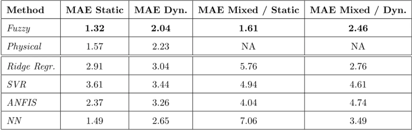
Table 1
Comparison of the prediction error (normalized MAE) of our fuzzy modelling com-ponent on various data sets, with physical model and with other data-driven mod-elling techniques (second part of table)
Method MAE Static MAE Dyn. MAE Mixed / Static MAE Mixed / Dyn.
Fuzzy 1.32 2.04 1.61 2.46 Physical 1.57 2.23 NA NA Ridge Regr. 2.91 3.04 5.76 2.76 SVR 3.61 3.44 4.94 4.61 ANFIS 2.37 3.26 4.04 4.74 NN 1.49 2.65 7.06 3.49
estimated and real measured NOx content in the emission significantly (in fact, achieving 5.50 MAE in case of static data tested on dynamic model, 6.06 MAE in case of dynamic tested on static model — compare with other values in Table 1). From this, we can conclude that mixed models trained from both dynamic and static data are necessary 1.) in order to circumvent time-intensive switches between two models and 2.) to provide reliable predictions.
A final comparison on the mean absolute error in numbers is presented in Ta-ble 1 for all data sets, the last column marks the corresponding figure. In the first column the modelling approach (fuzzy resp. physical modelling on static, dynamic or mixed data) is listed before the slash, whereas after the slash the type of test data is indicated. The error is demonstrated by the normalized version of MAE (normalized by the range of the NOx values). The latter shows the relative deviation in percent. The first part of this table is dedicated to the comparison between our fuzzy modelling approach and physical-oriented analytical models, following the error plots above. The second part (after the double line) shows the error achieved by four other data-driven modelling ap-proaches, namely ridge regression (robust linear regression by performing QR decomposition) [39] (available in statistics toolbox), support vector regression (SVR) [40,41] (usinglib-SVMimplementation),ANFIS (adaptive neuro-fuzzy inference systems) [42] (implemented in MATLAB’s fuzzy logic toolbox) and generalized regression neural networks [43] (available in MATLAB’s neural network toolbox). These are again applied within a best parameter grid search
scenario coupled with 10-fold cross-validation, where the optimal parameter setting (leading to the lowest CD error) is used for training the final model which is again evaluated with the separate test data set. The parameters to be steered are the number of inputs (= number of linear parameters) in case of ridge regression, the parameters C and γ in case of SVR, where the range of these are following the guidelines mentioned in the lib-SVM user documen-tation [44], the number of rules in case of ANFIS and the number of neurons (controlled by the spread) in case of generalized regression neural networks. From these error numbers in Table 1 (second column), we can conclude that our fuzzy modelling approach is out-performing all other data-driven mod-elling techniques significantly, no matter whether applied for static, mixed and dynamic data set (in most cases for static data more significantly than for dynamic data). The same performance problems arose for the other data-driven modelling approaches when training models on static data and testing them with dynamic data and vice versa, dropping MAE normalized by more than 100% (hence, we neglect these numbers in the second part of the table). Together with the aspect of providing rules with some interpretable quality and therefore gaining linguistic insight (see subsequent section), we can con-clude that fuzzy modelling with FLEXFIS is in fact a very good choice for a data-driven design of NOx prediction models.
4.3.3 Model Complexities and Computation Times
Table 2 shows the obtained model complexities of the final fuzzy models when trained on the whole set of training data by using the optimal parameter set-ting elicited during the 10-fold cross-validation coupled with best parameter grid search scenario. The second column demonstrates the number of inputs, finally used in the models (these were below 10 in all fuzzy modeling cases), the third column represents the number of rules in the final models — in the dynamic case this number turned out to be quite low: 11 rules were feasible for setting up a reliable model; for the physical models, the number of look-up tables are reported instead of the number of rules, for SVR the number of support vectors, for neural networks the number of neurons, summarized as ’structural elements’ in Column#3, as these are all responsible for the final degree of non-linearity/flexibility and transparency of the models. Compared to the other data-driven modelling techniques, our fuzzy approach could in large cases provide models with lower number of inputs and less structural components. An exception is the ANFIS approach, which could provide less complexity of the final achieved neuro-fuzzy model in case of dynamic data set (3 inputs, 8 rules compared to 8 inputs, 11 rules obtained with FLEX-FIS). However, the accuracy of the model suffers significantly (3.26 versus 2.04 normalized MAE in case of dynamic data). Another exception are the generalized regression neural network, which provide an optimal final model by using only two inputs (instead of 9 inFLEXFIS) in the case of mixed data
Table 2
Comparison of obtained model complexities (of the model trained based on the best parameter setting) and computation times needed in average for one model training step and in average for predicting one single sample, the latter representing the on-line prediction response
Modelling # of Inputs # of Structural Components Comp Time Training / Prediction in sec.
Fuzzy static 5 14 0.08 / 0.0006
Fuzzy dynamic 8 11 9.96 / 0.0045
Fuzzy mixed 9 22 10.07 / 0.0049
Physical static 7 17 NA
Physical dyn. 7 static + 1 NA
Ridge regression static 21 21 0.028 / 0.00039
Ridge regression dynamic 20 20 3.823 / 0.00039
Ridge regression mixed 16 16 3.89 / 0.00028
SVR static 15 23 0.18 / 0.00029 SVR dynamic 15 135 10.14 / 0.000465 SVR mixed 5 358 10.46 / 0.00083 ANFIS static 5 32 1.08 / 0.000126 ANFIS dynamic 3 8 15.00 / 0.000039 ANFIS mixed 6 64 164.00 / 0.0049 NN static 20 230 0.11 / 0.0011 NN dynamic 20 155 41.71 / 0.011 NN mixed 2 20 1.93 / 0.0043
set. However, it heavily suffers from model bias (7.06 normalized MAE ver-sus 1.61 in case of static data). Regarding computation times (last column in Table 2), all approaches are performing pretty fast, especially for predicting new samples; there were some problems withANFIS training approach when increasing the input dimensionality to above 5 in case of dynamic and mixed data sets (¿ 15000 training samples), as slowing down significantly during the learning phase — this can be explained by the exponential explosion of the number of rules. Some examples of fuzzy sets and rules for the dynamic case are shown in Figures 15 and 16, the variables were normalized to [0,1] before hand for comparison purpose in the rules consequents: higher absolute values indicate a higher impact of the variables in the corresponding local regions.
(a)(b)
Fig. 15. Fuzzy sets for the two input variables (from (a) to (b)) EGR (gas compo-sition at the intake manifold) andTint (intake gas temperature)
Rule 1: If
mf Is LOW And
EGR Is VLOW And
SOI Is LOW And
EGR·Fr Is MEDIUM And
Tint Is MEDIUM And
Then NOx = 0.0283*mf+0.1747*EGR +0.2998*SOI-0.033*EGR·Fr -0.0078*Tint+0.019 Rule 2: If mf Is HIGH And
EGR Is VLOW And
SOI Is MEDIUM And
EGR·Fr Is LOW And
Tint Is LOW Then NOx = 0.416*mf+0.868*EGR -0.883*SOI-2.65*EGR·Fr +0.066*Tint+0.841 Rule 3: If mf Is MEDIUM And
EGR Is HIGH And
SOI Is MEDIUM And EGR·Fr Is MEDIUM And
Tint Is HIGH Then NOx = 0.373*mf-0.121*EGR +0.027*SOI-0.341*EGR·Fr +0.026*Tint+0.16
Fig. 16. Three rule examples obtained with FLEXFIS for the static data set Also listed the computation times in the last column of Table 2: as we have used 135 training runs (for 135 knots in the grid), we took the average over all (final) training runs, leading to a value of around 10 seconds in the dynamic
data case (including 16936 training samples) and of 0.08 seconds in the static data case. The computation times for obtaining the prediction of one single sample with final achieved fuzzy model (corresponding to optimal parameter setting) are reported in the last column after the slash. In all cases, this value is below one millisecond, indicating that the fuzzy modeling methods can deal with quite fast on-line prediction scenarios.
5 Conclusions
In this paper, we presented an alternative to conventional NOx prediction models by training fuzzy models directly from measurement data, represent-ing static and dynamic operation modes. The used fuzzy systems modellrepresent-ing method was theFLEXFISapproach, which also offers the opportunity that the models are further updated, extended and improved during on-line mode with new incoming samples. The fuzzy models could slightly outperform physical-based models, no matter whether using static and dynamic data sets. Together with the aspects that
(1) it was also possible to set up a mixed model with high accuracy, which is able to predict new samples either from static or dynamic operation modes (such that no time-intensive distinction is necessary), and
(2) to have a kind of plug-and-play method available for setting up new models (in fact, the fuzzy models are trained and evaluated completely automatically from data)
(3) it was able to out-perform other data-driven (nearly plug-and-play) mod-elling techniques based on neuro-fuzzy and neural network architectures as well as support vector and ridge regression algorithms.
we can conclude that our fuzzy modelling component is in fact a reliable and good alternative to physical-based models, which for a new engine require time-intensive re-adjustments, in worst case even re-development phases.
Acknowledgement
This work was supported by the Upper Austrian Technology and Research Promotion. This publication reflects only the author’s view. Furthermore, we acknowledge PSA for providing the engine and partially supporting our inves-tigation. Special thanks are given to PO Calendini, P Gaillard and C. Bares at the Diesel Engine Control Department.
References
[1] J. Riesco, F. Payri, J. B. S. Molina, Reduction of pollutant emissions in a HD diesel engine by adjustment of injection parameters, boost pressure and EGR, SAE paper 2003-01-0343.
[2] R. Basshuysen, F. Schaefer, Internal combustion engine handbook: basics, components, systems, and perspectives, SAE International, Warrendale, PA, 2004.
[3] Y. Zeldovich, The oxidation of nitrogen in combustion and explosions, Acta Physicochemica 21 (1946) 577–628.
[4] C. Fenimore, Formation of nitric oxide in premixed hydrocarbon flames, in: Proc. 13th Symposium (International) on Combustion, Pittsburgh, PA, 1971, pp. 373–379.
[5] J. Arr`egle, J. L´opez, C. Guardiola, C. Monin, Sensitivity study of a nox estimation model for on-board applications, SAE paper 2008-01-0640.
[6] R. Moos, A brief overview on automotive exhaust gas sensors based on electroceramics, International Journal of Applied Ceramic Technology 2 (5) (2005) 401–413.
[7] U. Gartner, G. Hohenberg, H. Daudel, H. Oelschlegel, Development and application of a semi-empirical nox model to various hd diesel engines, in: Proc. of THIESEL, Valencia, Spain, 2002, pp. 487–506.
[8] T. Kamimoto, H. Kobayashi, Combustion processes in diesel engines, Progress in Energy and Combustion Science 17 (1991) 163–189.
[9] G. Weisser, Modelling of combustion and nitric-oxide formation for medium-speed di diesel engines: a comparative evaluation of zero- and three-dimensional approaches, Ph.D. thesis, Swiss Federal Institute of Technology (Zuerich 2001). [10] E. Lughofer, Extensions of vector quantization for incremental clustering,
Pattern Recognition 41 (3) (2008) 995–1011.
[11] J. Galindo, H. Climent, C. Guardiola, J. Dom´enech, Strategies for improving the mode transition in a sequential parallel turbocharged automotive diesel engine, International Journal of Automotive Technology 10 (2) (2009) 141–149. [12] J. Galindo, H. Climent, C. Guardiola, A. Tiseira, J. Portalier, Assessment of a
sequentially turbocharged diesel engine on real-life driving cycles, International Journal of Vehicle Design 49 (1-3) (2009) 214–234.
[13] J. Desantes, J. Galindo, C. Guardiola, V. Dolz, Air mass flow estimation in turbocharged diesel engines from in-cylinder pressure measurement, Experimental Thermal and Fluid Science 34 (1) (2010) 37–47.
[14] T. Takagi, M. Sugeno, Fuzzy identification of systems and its applications to modeling and control, IEEE Trans. on Systems, Man and Cybernetics 15 (1) (1985) 116–132.
[15] L. Wang, J. Mendel, Fuzzy basis functions, universal approximation and orthogonal least-squares learning, IEEE Trans. Neural Networks 3 (5) (1992) 807–814.
[16] L. Wang, Fuzzy systems are universal approximators, in: Proc. 1st IEEE Conf. Fuzzy Systems, San Diego, CA, 1992, pp. 1163–1169.
[17] S. Yan, Z. Sun, Universal approximation for takagi-sugeno fuzzy systems using dynamically constructive method-miso cases, in: Proceedings of the IEEE 22nd International Symposium on Intelligent Control, Singapore, 2007, pp. 150–155. [18] J. Casillas, O. Cordon, F. Herrera, L. Magdalena, Interpretability Issues in
Fuzzy Modeling, Springer Verlag, Berlin Heidelberg, 2003.
[19] M. Galea, Q.-Shen, Linguistic hedges for ant-generated rules, in: Proceedings of the 2006 IEEE International Conference on Fuzzy Systems, Vancouver, Canada, 2006, pp. 1973–1980.
[20] J. M. Blazquez, Q. Shen, Regaining comprehensibility of approximative fuzzy models via the use of linguistic hedges, in: J. Casillas, O. Cord´on, F. Herrera, L. Magdalena (Eds.), Interpretability Issues in Fuzzy Modeling, Vol. 128 of Studies in Fuzziness and Soft Computing, Springer, Berlin, 2003, pp. 25–53. [21] A. Piegat, Fuzzy Modeling and Control, Physica Verlag, Springer Verlag
Company, Heidelberg, New York, 2001.
[22] E. Lughofer, S. Kindermann, Rule weight optimization and feature selection in fuzzy systems with sparsity constraints, in: Proceedings of the IFSA/EUSFLAT 2009 conference, Lisbon, Portugal, 2009, pp. 950–956.
[23] J. Yen, L. Wang, C. Gillespie, Improving the interpretability of TSK fuzzy models by combining global learning and local learning, IEEE Trans. on Fuzzy Systems 6 (4) (1998) 530–537.
[24] R. Gray, Vector quantization, IEEE ASSP Magazine (1984) 4–29.
[25] E. Lughofer, FLEXFIS: A robust incremental learning approach for evolving TS fuzzy models, IEEE Trans. on Fuzzy Systems 16 (6) (2008) 1393–1410. [26] S. Qin, W. Li, H. Yue, Recursive PCA for adaptive process monitoring, Journal
of Process Control 10 (2000) 471–486.
[27] E. Lughofer, Evolving vector quantization for classification of on-line data streams, in: Proc. of the Conference on Computational Intelligence for Modelling, Control and Automation (CIMCA 2008), Vienna, Austria, 2008, pp. 780–786.
[28] E. Lughofer, Evolving Fuzzy Models — Incremental Learning, Interpretability and Stability Issues, Applications, VDM Verlag Dr. M¨uller, Saarbr¨ucken, 2008. [29] A. Tikhonov, V. Arsenin, Solutions of ill-posed problems, Winston & Sonst,
[30] F. Bauer, M. Lukas, Comparing parameter choice methods for regularization of ill-posed problems, Inverse ProblemsSubmitted.
[31] F. Bauer, Some considerations concerning regularization and parameter choice algorithms, Inverse Problems 23 (2007) 837 – 858.
[32] E. Lughofer, S. Kindermann, Improving the robustness of data-driven fuzzy systems with regularization, in: Proc. of the IEEE World Congress on Computational Intelligence (WCCI) 2008, Hongkong, 2008, pp. 703–709. [33] L. Ljung, System Identification: Theory for the User, Prentice Hall PTR, Prentic
Hall Inc., Upper Saddle River, New Jersey 07458, 1999.
[34] L. Eriksson, J. Wahlstr¨om, M. Klein, Automotive Model Predictive Control: Models, Methods and Applications (Eds: L. del Re, F. Allg¨ower, L. Glielmo, C. Guardiola, and I. Kolmanovsky), Springer Verlag, 2010, Ch. Physical modeling of turbocharged engines and parameter identification, pp. 59–79.
[35] J. Arr`egle, J. L´opez, C. Guardiola, C. Monin, Automotive Model Predictive Control: Models, Methods and Applications (Eds: L. del Re, F. Allg¨ower, L. Glielmo, C. Guardiola, and I. Kolmanovsky), Springer Verlag, 2010, Ch. On board NOx prediction in diesel engines. A physical approach, pp. 27–39. [36] M. Stone, Cross-validatory choice and assessment of statistical predictions,
Journal of the Royal Statistical Society 36 (1974) 111–147.
[37] W. Groißb¨ock, E. Lughofer, E. Klement, A comparison of variable selection methods with the main focus on orthogonalization, in: M. Lop´ez-D´ıaz, M. Gil, P. Grzegorzewski, O. Hryniewicz, J. Lawry (Eds.), Soft Methodology and Random Information Systems, Advances in Soft Computing, Springer, Berlin, Heidelberg, New York, 2004, pp. 479–486.
[38] T. Hastie, R. Tibshirani, J. Friedman, The Elements of Statistical Learning: Data Mining, Inference and Prediction, Springer Verlag, New York, Berlin, Heidelberg, Germany, 2001.
[39] N. Draper, H. Smith, Applied Regression Analysis. Probability and Mathematical Statistics, John Wiley & Sons, New York, 1981.
[40] B. Sch¨olkopf, A. Smola, Learning with Kernels - Support Vector Machines, Regularization, Optimization and Beyond, MIT Press, London, England, 2002. [41] V. Vapnik, Statistical Learning Theory, Wiley and Sons, New York, 1998. [42] J.-S. Jang, ANFIS: Adaptive-network-based fuzzy inference systems, IEEE
Trans. Syst. Man Cybern. 23 (1993) 665–685.
[43] P. Wasserman, Advanced Methods in Neural Computing, Van Nostrand Reinhold, New York, 1993.
[44] C.-W. Hsu, C.-C. Chang, , C.-J. Lin, A practical guide to support vector classification (2006).


![Automatisk orddeling (Automatic word splitting) [In Danish]](data:image/gif;base64,R0lGODlhAQABAIAAAP///wAAACH5BAEAAAAALAAAAAABAAEAAAICRAEAOw==)