University of Central Florida University of Central Florida
STARS
STARS
Electronic Theses and Dissertations, 2004-2019
2013
Investigating The Relationship Between Adverse Events And
Investigating The Relationship Between Adverse Events And
Infrastructure Development In An Active War Theater Using Soft
Infrastructure Development In An Active War Theater Using Soft
Computing Techniques
Computing Techniques
Erman CakitUniversity of Central Florida
Part of the Industrial Engineering Commons
Find similar works at: https://stars.library.ucf.edu/etd
University of Central Florida Libraries http://library.ucf.edu
This Doctoral Dissertation (Open Access) is brought to you for free and open access by STARS. It has been accepted for inclusion in Electronic Theses and Dissertations, 2004-2019 by an authorized administrator of STARS. For more information, please contact [email protected].
STARS Citation STARS Citation
Cakit, Erman, "Investigating The Relationship Between Adverse Events And Infrastructure Development In An Active War Theater Using Soft Computing Techniques" (2013). Electronic Theses and Dissertations, 2004-2019. 2611.
INVESTIGATING THE RELATIONSHIP BETWEEN ADVERSE EVENTS AND
INFRASTRUCTURE DEVELOPMENT IN AN ACTIVE WAR THEATER USING SOFT COMPUTING TECHNIQUES
by
ERMAN ÇAKIT
B.S. Industrial Engineering, University of Gaziantep, Turkey, 2006 M.S. Industrial Engineering, Çukurova University, Turkey, 2008
A dissertation submitted in partial fulfillment of the requirements for the degree of Doctor of Philosophy
in the Department of Industrial Engineering and Management Systems in the College of Engineering and Computer Science
at the University of Central Florida Orlando, Florida
Summer Term 2013
ii
iii
ABSTRACT
The military recently recognized the importance of taking sociocultural factors into consideration. Therefore, Human Social Culture Behavior (HSCB) modeling has been getting much attention in current and future operational requirements to successfully understand the effects of social and cultural factors on human behavior. There are different kinds of modeling approaches to the data that are being used in this field and so far none of them has been widely accepted. HSCB modeling needs the capability to represent complex, ill-defined, and imprecise concepts, and soft computing modeling can deal with these concepts.
There is currently no study on the use of any computational methodology for representing the relationship between adverse events and infrastructure development investments in an active war theater. This study investigates the relationship between adverse events and infrastructure development projects in an active war theater using soft computing techniques including fuzzy inference systems (FIS), artificial neural networks (ANNs), and adaptive neuro-fuzzy inference systems (ANFIS) that directly benefits from their accuracy in prediction applications. Fourteen developmental and economic improvement project types were selected based on allocated budget values and a number of projects at different time periods, urban and rural population density, and total adverse event numbers at previous month selected as independent variables. A total of four outputs reflecting the adverse events in terms of the number of people killed, wounded, hijacked, and total number of adverse events has been estimated. For each model, the data was grouped for training and testing as follows: years between 2004 and 2009 (for training purpose) and year
iv
and the country was divided into seven regions for analysis purposes. Performance of each model was investigated and compared to all other models with the calculated mean absolute error (MAE) values and the prediction accuracy within ±1 error range (difference between actual and predicted value). Furthermore, sensitivity analysis was performed to determine the effects of input values on dependent variables and to rank the top ten input parameters in order of importance.
According to the the results obtained, it was concluded that the ANNs, FIS, and ANFIS are useful modeling techniques for predicting the number of adverse events based on historical development or economic projects’ data. When the model accuracy was calculated based on the MAE for each of the models, the ANN had better predictive accuracy than FIS and ANFIS models in general as demonstrated by experimental results. The percentages of prediction accuracy with values found within ±1 error range around 90%. The sensitivity analysis results show that the importance of economic development projects varies based on the regions, population density, and occurrence of adverse events in Afghanistan. For the purpose of allocating resources and development of regions, the results can be summarized by examining the relationship between adverse events and infrastructure development in an active war theater; emphasis was on predicting the occurrence of events and assessing the potential impact of regional infrastructure development efforts on reducing number of such events.
v
Throughout my work, two special people have always been there during those years of hard times. This dissertation is dedicated to my parents, Ayşe and Şükrü Çakıt, for their endless love,
vi
ACKNOWLEDGMENTS
I would like to express my deepest gratitude to my advisor Dr. Waldemar Karwowski. This dissertation would not have been finished without his guidance and persistent support. My decision to become an academician was sparked after I met with him. It is my sincere hope that I affect students in my professional life as profoundly as he has affected me.
I would like to thank my committee members, Dr. Thompson, Dr. Lee, and Dr. Mikusinski for being in committee and for their time and invaluable feedback.
I would like to thank Dr. Ahram for his support. During the research meetings, I appreciate his invaluable and motivational comments to help me progress in research.
I would like to thank Republic of Turkey Ministry of National Education for their financial support and encouragement during my graduate study.
Finally, I would like to thank Office of Naval Research Human Social Cultural Behavioral Program. This dissertation was supported in part by Grant No. 1052339, Complex Systems Engineering for Rapid Computational Socio-Cultural Network Analysis, from the Office of Naval Research.
vii
TABLE OF CONTENTS
LIST OF FIGURES ... xi
LIST OF TABLES ... xxvi
LIST OF ABBREVIATIONS ... xxxv
CHAPTER I: INTRODUCTION ... 1
1.1 From War to Nation-Building in Afghanistan ... 1
1.2 Human Social Culture Behavior (HSCB) Modeling ... 5
1.3 Problem Statement ... 7
1.4 Research Gap... 8
1.5 Research Objectives ... 8
1.6 Research Questions ... 8
1.7 Study Design ... 9
CHAPTER II: LITERATURE REVIEW ... 11
2.1 Challenges and General Modeling Approaches ... 11
2.2 Spatial Statistics ... 12
2.3 Soft Computing Techniques and Applications... 15
2.3.1 Fuzzy Clustering ... 16
viii
2.5 Agent-Based Approaches ... 18
2.6 Linguistic Pattern Analysis ... 20
CHAPTER III: METHODOLOGY ... 21
3.1 Soft-Computing Techniques ... 21
3.1.1 Artificial Neural Networks ... 23
3.1.1.1 The Architecture of ANNs ... 25
3.1.1.2 Network Training Algorithm ... 29
3.1.1.3 Transfer (Activation) functions... 30
3.1.1.4 Data Normalization ... 32
3.1.2 Fuzzy Sets ... 35
3.1.2.1 Membership Functions... 36
3.1.2.2 Fuzzy Systems ... 37
3.1.2.3 Data Clustering ... 40
3.1.3 Adaptive Neuro-Fuzzy Inference Systems (ANFIS) ... 44
3.1.3.1 ANFIS Input Selection ... 47
3.2 The dataset... 49
3.3 Performance Metrics ... 54
CHAPTER IV: RESULTS ... 55
ix
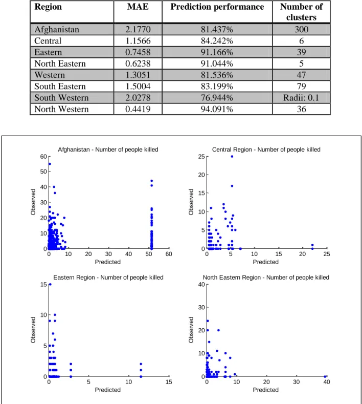
4.1.1 Prediction of number of people killed ... 59
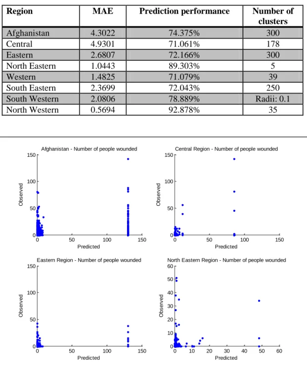
4.1.2 Prediction of number of people wounded... 63
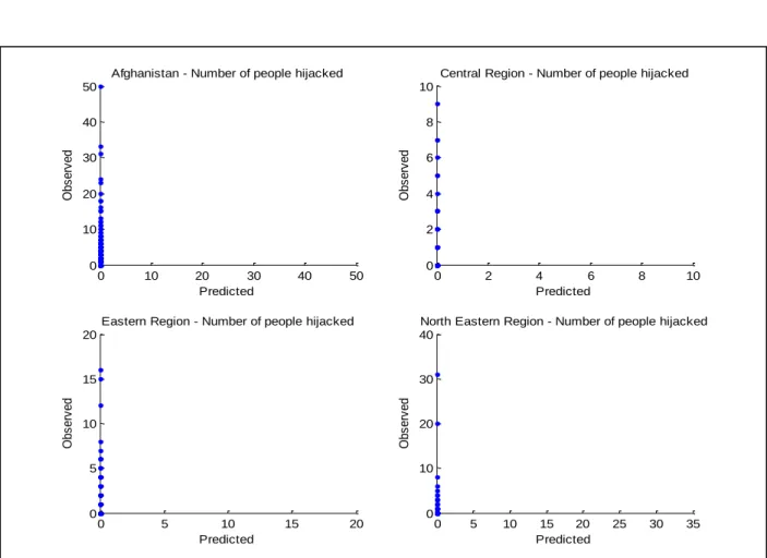
4.1.3 Prediction of number of people hijacked ... 67
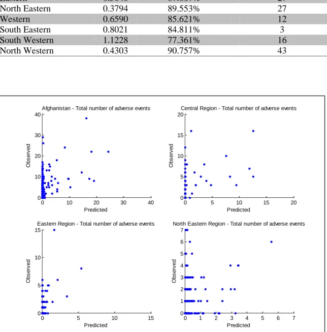
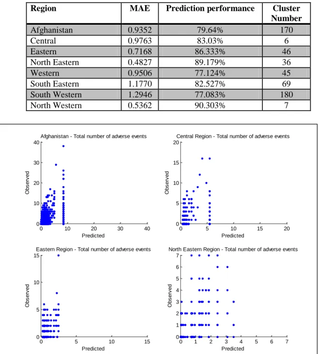
4.1.4 Prediction of total number of adverse events ... 71
4.2 FIS Model Development ... 75
4.2.1 Prediction of number of people killed ... 77
4.2.2 Prediction of number of people wounded... 81
4.2.3 Prediction of number of people hijacked ... 85
4.2.4 Prediction of total number of adverse events ... 89
4.3 ANFIS Model Development ... 94
4.3.1 Prediction of number of people killed ... 97
4.3.2 Prediction of number of people wounded... 100
4.3.3 Prediction of number of people hijacked ... 104
4.3.4 Prediction of total number of adverse events ... 108
4.4 Performance Comparison of Models... 112
4.5 Sensitivity Analysis ... 126
CHAPTER V: CONCLUSION... 148
5.1. Study Contributions... 148
x
5.3 Study Limitations and Future Work ... 149
5.3.1 Data Limitations ... 149
5.3.2 ANN Model Limitations ... 150
5.3.3 FIS Model Limitations... 150
5.3.4 ANFIS Model Limitations ... 151
APPENDIX A: SNAPSHOT OF PARTIAL DATASET ... 152
APPENDIX B: CORRELATION RESULTS ... 162
APPENDIX C: MATLAB CODE FOR EACH METHODOLOGY ... 171
APPENDIX D: MAP REPRESENTATION OF MONTHLY PREDICTED AND OBSERVED VALUES FOR ENTIRE AFGHANISTAN ... 177
APPENDIX E: MONTHLY MAE AND PERCENTAGE VALUES ... 225
APPENDIX F: SENSITIVITY ANALYSIS RESULTS FOR ALL RANKED INPUT VALUES ... 242
APPENDIX G: SENSITIVITY ANALYSIS GRAPHS FOR THE TOP TWO RANKED VALUES ... 309
xi
LIST OF FIGURES
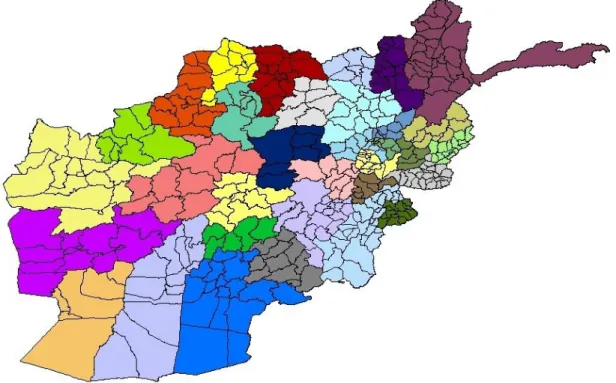
Figure 1: A map of the districts which are color grouped by province ... 1
Figure 2: Contrasting Conventional and Irregular Warfare ... 6
Figure 3: Common steps for all three methodologies ... 10
Figure 4: Hybrid approaches and the main components of Soft Computing ... 22
Figure 5: General model framework used in this research ... 23
Figure 6: Illustration of an artificial neural network ... 24
Figure 7: ANN architectures for each category ... 26
Figure 8: ANN learning process ... 27
Figure 9: Architecture of a feed-forward multilayered neural network ... 28
Figure 10: Log-sigmoid transfer function ... 31
Figure 11: Hyperbolic tangent transfer function ... 32
Figure 12: MATLAB normalization code ... 33
Figure 13: ANN flow diagram used in this study ... 34
Figure 14: Examples of common membership functions ... 36
Figure 15: A framework of fuzzy system ... 37
Figure 16: Fuzzy clustering example ... 40
Figure 17: FIS flow diagram used in this study ... 43
Figure 18: ANFIS architecture... 45
xii
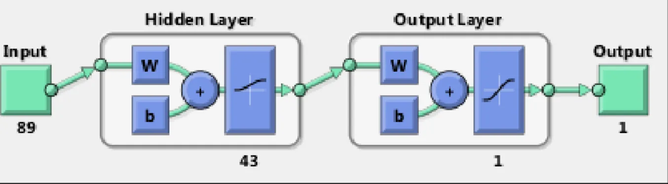
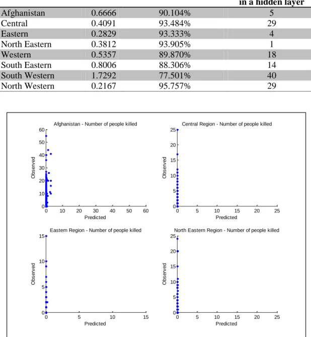
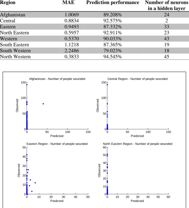
Figure 20: Year, month, province, district, and region info of partial training dataset ... 50 Figure 21: Regions of Afghanistan ... 53 Figure 22: Illustration of ANN model with forty-three neurons in a hidden layer for eighty-nine input parameters ... 58 Figure 23: ANN predicted and observed values of number of people killed for Afghanistan, central, eastern, and north eastern regions ... 62 Figure 24: ANN predicted and observed values of number of people killed for north western, south eastern, south western, and western regions ... 63 Figure 25: ANN predicted and observed values of number of people wounded for Afghanistan, central, eastern, and north eastern regions ... 66 Figure 26: ANN predicted and observed values of number of people wounded for north western, south eastern, south western, and western regions ... 67 Figure 27: ANN predicted and observed values of number of people hijacked for Afghanistan, central, eastern, and north eastern regions ... 70 Figure 28: ANN predicted and observed values of number of people hijacked for north western, south eastern, south western, and western regions ... 71 Figure 29: ANN predicted and observed values of number of total adverse events for
Afghanistan, central, eastern, and north eastern regions ... 74 Figure 30: ANN predicted and observed values of number of total adverse events for north western, south eastern, south western, and western regions ... 75 Figure 31: Illustration of membership functions when number of clusters equals to six ... 76 Figure 32: Illustration of rule number when number of clusters equals to six ... 77
xiii
Figure 33: FIS predicted and observed values of number of people killed for Afghanistan,
central, eastern, and north eastern regions ... 80 Figure 34: FIS predicted and observed values of number of people killed for north western, south eastern, south western, and western regions ... 81 Figure 35: FIS predicted and observed values of number of people wounded for Afghanistan, central, eastern, and north eastern regions ... 84 Figure 36: FIS predicted and observed values of number of people wounded for north western, south eastern, south western, and western regions ... 85 Figure 37: FIS predicted and observed values of number of people hijacked for Afghanistan, central, eastern, and north eastern regions ... 88 Figure 38: FIS predicted and observed values of number of people hijacked for north western, south eastern, south western, and western regions ... 89 Figure 39: FIS predicted and observed values of total number of adverse events for Afghanistan, central, eastern, and north eastern region... 92 Figure 40: FIS predicted and observed values of total number of adverse events for north
western, south eastern, south western, and western regions ... 93 Figure 41: Illustration of every input variable's influence on number of people killed in
Afghanistan ... 96 Figure 42: ANFIS predicted and observed values of number of people killed for Afghanistan, central, eastern, and north eastern regions ... 99 Figure 43: ANFIS predicted and observed values of number of people killed for north western, south eastern, south western, and western regions ... 100
xiv
Figure 44: ANFIS predicted and observed values of number of people wounded for Afghanistan,
central, eastern, and north eastern regions ... 103
Figure 45: ANFIS predicted and observed values of number of people wounded for north western, south eastern, south western, and western regions ... 104
Figure 46: ANFIS predicted and observed values of number of people hijacked for Afghanistan and central, eastern, and north eastern regions ... 107
Figure 47: ANFIS predicted and observed values of number of people hijacked for north western, south eastern, south western, and western regions ... 108
Figure 48: ANFIS predicted and observed values of total number of adverse events for Afghanistan, and central, eastern, and north eastern regions ... 111
Figure 49: ANFIS predicted and observed values of total number of adverse events for north western, south eastern, south western, and western regions ... 112
Figure 50: MAE values of predicted values for Afghanistan ... 113
Figure 51: Percentage values of model prediction accuracy for Afghanistan ... 113
Figure 52: MAE values of predicted values for central region ... 114
Figure 53: Percentage values of model prediction accuracy for central region ... 115
Figure 54: MAE values of predicted values for eastern region ... 115
Figure 55: Percentage values of model prediction accuracy for eastern region ... 116
Figure 56: MAE values of predicted values for north eastern region ... 117
Figure 57: Percentage values of model prediction accuracy for north eastern region ... 117
Figure 58: MAE values of predicted values for western region ... 118
xv
Figure 60: MAE values of predicted values for south eastern region... 119
Figure 61: Percentage values of model prediction accuracy for south eastern region ... 120
Figure 62: MAE values of predicted values for south western region ... 121
Figure 63: Percentage values of model prediction accuracy for south western region ... 121
Figure 64: MAE values of predicted values for north western region ... 122
Figure 65: Percentage values of model prediction accuracy for north western region ... 123
Figure 66: Predicted and observed values of number of people killed for each district in January 2010... 125
Figure 67: Sensitivity analysis on trained ANN ... 126
Figure 68: The effect of the first ranked independent variable on number of people wounded in Eastern region ... 139
Figure 69: The effect of the second ranked independent variable on number of people wounded in Eastern region ... 140
Figure 70: Partial budget info of fourteen projects at year t-2 ... 153
Figure 71: Partial aid number info of fourteen projects at year t-2 ... 154
Figure 72: Partial budget info of fourteen projects at year t-1 ... 155
Figure 73: Partial aid number info of fourteen projects at year t-1 ... 156
Figure 74: Partial budget info of fourteen projects at year t ... 157
Figure 75: Partial aid number info of fourteen projects at year t ... 158
Figure 76: Partial urban and rural population density info for male and female ... 159
Figure 77: Partial dataset info of number of people killed, wounded, hijacked and total number of adverse events at month t-1... 160
xvi
Figure 78: Partial dataset info of output values ... 161 Figure 79: Predicted and observed values of number of people killed for each district in February 2010... 178 Figure 80: Predicted and observed values of number of people killed for each district in March 2010... 179 Figure 81: Predicted and observed values of number of people killed for each district in April 2010... 180 Figure 82: Predicted and observed values of number of people killed for each district in May 2010... 181 Figure 83: Predicted and observed values of number of people killed for each district in June 2010... 182 Figure 84: Predicted and observed values of number of people killed for each district in July 2010... 183 Figure 85: Predicted and observed values of number of people killed for each district in August 2010... 184 Figure 86: Predicted and observed values of number of people killed for each district in
September 2010 ... 185 Figure 87: Predicted and observed values of number of people killed for each district in October 2010... 186 Figure 88: Predicted and observed values of number of people killed for each district in
xvii
Figure 89: Predicted and observed values of number of people killed for each district in
December 2010 ... 188 Figure 90: Predicted and observed values of number of people wounded for each district in January 2010 ... 189 Figure 91: Predicted and observed values of number of people wounded for each district in February 2010 ... 190 Figure 92: Predicted and observed values of number of people wounded for each district in March 2010 ... 191 Figure 93: Predicted and observed values of number of people wounded for each district in April 2010... 192 Figure 94: Predicted and observed values of number of people wounded for each district in May 2010... 193 Figure 95: Predicted and observed values of number of people wounded for each district in June 2010... 194 Figure 96: Predicted and observed values of number of people wounded for each district in July 2010... 195 Figure 97: Predicted and observed values of number of people wounded for each district in August 2010 ... 196 Figure 98: Predicted and observed values of number of people wounded for each district in September 2010 ... 197 Figure 99: Predicted and observed values of number of people wounded for each district in October 2010 ... 198
xviii
Figure 100: Predicted and observed values of number of people wounded for each district in November 2010 ... 199 Figure 101: Predicted and observed values of number of people wounded for each district in December 2010 ... 200 Figure 102: Predicted and observed values of number of people hijacked for each district in January 2010 ... 201 Figure 103: Predicted and observed values of number of people hijacked for each district in February 2010 ... 202 Figure 104: Predicted and observed values of number of people hijacked for each district in March 2010 ... 203 Figure 105: Predicted and observed values of number of people hijacked for each district in April 2010... 204 Figure 106: Predicted and observed values of number of people hijacked for each district in May 2010... 205 Figure 107: Predicted and observed values of number of people hijacked for each district in June 2010... 206 Figure 108: Predicted and observed values of number of people hijacked for each district in July 2010... 207 Figure 109: Predicted and observed values of number of people hijacked for each district in August 2010 ... 208 Figure 110: Predicted and observed values of number of people hijacked for each district in September 2010 ... 209
xix
Figure 111: Predicted and observed values of number of people hijacked for each district in October 2010 ... 210 Figure 112: Predicted and observed values of number of people hijacked for each district in November 2010 ... 211 Figure 113: Predicted and observed values of number of people hijacked for each district in December 2010 ... 212 Figure 114: Predicted and observed values of number of total adverse events for each district in January 2010 ... 213 Figure 115: Predicted and observed values of number of total adverse events for each district in February 2010 ... 214 Figure 116: Predicted and observed values of number of total adverse events for each district in March 2010 ... 215 Figure 117: Predicted and observed values of number of total adverse events for each district in April 2010 ... 216 Figure 118: Predicted and observed values of number of total adverse events for each district in May 2010 ... 217 Figure 119: Predicted and observed values of number of total adverse events for each district in June 2010 ... 218 Figure 120: Predicted and observed values of number of total adverse events for each district in July 2010 ... 219 Figure 121: Predicted and observed values of number of total adverse events for each district in August 2010 ... 220
xx
Figure 122: Predicted and observed values of number of total adverse events for each district in September 2010 ... 221 Figure 123: Predicted and observed values of number of total adverse events for each district in October 2010 ... 222 Figure 124: Predicted and observed values of number of total adverse events for each district in November 2010 ... 223 Figure 125: Predicted and observed values of number of total adverse events for each district in December 2010 ... 224 Figure 126: The effect of the first ranked independent variable on number of people killed in Central region... 310 Figure 127: The effect of the second ranked independent variable on number of people killed in Central region... 310 Figure 128: The effect of the first ranked independent variable on number of people wounded in Central region... 311 Figure 129: The effect of the second ranked independent variable on number of people wounded in Central region ... 311 Figure 130: The effect of the first ranked independent variable on number of people hijacked in Central region... 312 Figure 131: The effect of the second ranked independent variable on number of people hijacked in Central region ... 312 Figure 132: The effect of the first ranked independent variable on total number of adverse events in Central region ... 313
xxi
Figure 133: The effect of the second ranked independent variable on total number of adverse events in Central region ... 313 Figure 134: The effect of the first ranked independent variable on number of people killed in Eastern region ... 314 Figure 135: The effect of the second ranked independent variable on number of people killed in Eastern region ... 314 Figure 136: The effect of the first ranked independent variable on number of people hijacked in Eastern region ... 315 Figure 137: The effect of the second ranked independent variable on number of people hijacked in Eastern region ... 315 Figure 138: The effect of the first ranked independent variable on total number of adverse events in Eastern region ... 316 Figure 139: The effect of the second ranked independent variable on total number of adverse events in Eastern region ... 316 Figure 140: The effect of the first ranked independent variable on number of people killed in North Eastern region ... 317 Figure 141: The effect of the second ranked independent variable on number of people killed in North Eastern region ... 317 Figure 142: The effect of the first ranked independent variable on number of people wounded in North Eastern region ... 318 Figure 143: The effect of the second ranked independent variable on number of people wounded in North Eastern region ... 318
xxii
Figure 144: The effect of the first ranked independent variable on number of people hijacked in North Eastern region ... 319 Figure 145: The effect of the second ranked independent variable on number of people hijacked in North Eastern region ... 319 Figure 146: The effect of the first ranked independent variable on total number of adverse events in North Eastern region ... 320 Figure 147: The effect of the second ranked independent variable on total number of adverse events in North Eastern region ... 320 Figure 148: The effect of the first ranked independent variable on number of people killed in North Western region ... 321 Figure 149: The effect of the second ranked independent variable on number of people killed in North Western region ... 321 Figure 150: The effect of the first ranked independent variable on number of people wounded in North Western region ... 322 Figure 151: The effect of the second ranked independent variable on number of people wounded in North Western region... 322 Figure 152: The effect of the first ranked independent variable on number of people hijacked in North Western region ... 323 Figure 153: The effect of the second ranked independent variable on number of people hijacked in North Western region... 323 Figure 154: The effect of the first ranked independent variable on total number of adverse events in North Western region... 324
xxiii
Figure 155: The effect of the second ranked independent variable on total number of adverse events in North Western region ... 324 Figure 156: The effect of the first ranked independent variable on number of people killed in South Eastern region ... 325 Figure 157: The effect of the second ranked independent variable on number of people killed in South Eastern region ... 325 Figure 158: The effect of the first ranked independent variable on number of people wounded in South Eastern region ... 326 Figure 159: The effect of the second ranked independent variable on number of people wounded in South Eastern region ... 326 Figure 160: The effect of the first ranked independent variable on number of people hijacked in South Eastern region ... 327 Figure 161: The effect of the second ranked independent variable on number of people hijacked in South Eastern region ... 327 Figure 162: The effect of the first ranked independent variable on total number of adverse events in South Eastern region ... 328 Figure 163: The effect of the second ranked independent variable on total number of adverse events in South Eastern region ... 328 Figure 164: The effect of the first ranked independent variable on number of people killed in South Western region ... 329 Figure 165: The effect of the second ranked independent variable on number of people killed in South Western region ... 329
xxiv
Figure 166: The effect of the first ranked independent variable on number of people wounded in South Western region ... 330 Figure 167: The effect of the second ranked independent variable on number of people wounded in South Western region... 330 Figure 168: The effect of the first ranked independent variable on number of people hijacked in South Western region ... 331 Figure 169: The effect of the second ranked independent variable on number of people hijacked in South Western region... 331 Figure 170: The effect of the first ranked independent variable on total number of adverse events in South Western region... 332 Figure 171: The effect of the second ranked independent variable on total number of adverse events in South Western region ... 332 Figure 172: The effect of the first ranked independent variable on number of people killed in Western region ... 333 Figure 173: The effect of the second ranked independent variable on number of people killed in Western region ... 333 Figure 174: The effect of the first ranked independent variable on number of people wounded in Western region ... 334 Figure 175: The effect of the second ranked independent variable on number of people wounded in Western region ... 334 Figure 176: The effect of the first ranked independent variable on number of people hijacked in Western region ... 335
xxv
Figure 177: The effect of the second ranked independent variable on number of people hijacked in Western region ... 335 Figure 178: The effect of the first ranked independent variable on total number of adverse events in Western region ... 336 Figure 179: The effect of the second ranked independent variable on total number of adverse events in Western region ... 336
xxvi
LIST OF TABLES
Table 1: The milestones of U.S. War in Afghanistan ... 3 Table 2: Similarities between the components of ANNs and BNNs ... 25 Table 3: Comparison of Fuzzy Sets and Crisp Sets ... 35 Table 4. Main properties of neural network and fuzzy systems ... 44 Table 5: The variables used in model construction ... 51 Table 6: Empirical training dataset for years between 2004 and 2009 ... 52 Table 7: Empirical testing dataset for 2010 ... 52 Table 8: Province and district info for each region ... 53 Table 9: Percentage values of training and testing records for each region ... 55 Table 10: Number of people killed – ANN best configuration highlighted for each region based on number of neurons in a hidden layer... 60 Table 11: ANN best model configuration for number of people killed in each region ... 62 Table 12: Number of people wounded – ANN best configuration highlighted for each region based on number of neurons in a hidden layer ... 64 Table 13: ANN best model configuration for number of people wounded in each region ... 66 Table 14: Number of people hijacked – ANN best configuration highlighted for each region based on number of neurons in a hidden layer ... 68 Table 15: ANN best model configuration for number of people hijacked in each region ... 70 Table 16: Total number of adverse events – ANN best configuration highlighted for each region based on number of neurons in a hidden layer ... 72
xxvii
Table 17: ANN best model configuration for total number of adverse events in each region ... 74 Table 18: Number of people killed – FIS best configuration for each region based on number of cluster ... 78 Table 19: FIS best model configuration for number of people killed in each region ... 80 Table 20: Number of people wounded – FIS best configuration for each region based on number of cluster... 82 Table 21: FIS best model configuration for number of people wounded in each region ... 84 Table 22: Number of people hijacked – FIS best configuration for each region based on number of cluster... 86 Table 23: FIS best model configuration for number of people hijacked in each region ... 88 Table 24: Total number of adverse events – FIS best configuration for each region based on number of cluster ... 90 Table 25: FIS best model configuration for total number of adverse events in each region ... 92 Table 26: Input variable and corresponding code ... 95 Table 27: Selected two inputs for each dependent variable and region ... 96 Table 28: Number of people killed– ANFIS best configuration for each region based on
membership function type and its number ... 97 Table 29: ANFIS best model configuration for number of people killed in each region ... 99 Table 30: Number of people wounded– ANFIS best configuration for each region based on membership function type and its number ... 101 Table 31: ANFIS best model configuration for number of people wounded in each region ... 103
xxviii
Table 32: Number of people hijacked– ANFIS best configuration for each region based on membership function type and its number ... 105 Table 33: ANFIS best model configuration for number of people hijacked in each region ... 107 Table 34: Total number of adverse events – ANFIS best configuration for each region based on membership function type and its number ... 109 Table 35: ANFIS best model configuration for total number of adverse events in each region 111 Table 36: Best prediction model for each region and dependent variable based on MAE values ... 124 Table 37: The sensitivity rank of all input values for number of people killed in central region127 Table 38: The rank of inputs and their effect on dependent variables of central region ... 132 Table 39: The rank of inputs and their effect on dependent variables of eastern region ... 133 Table 40: The rank of inputs and their effect on dependent variables of north-eastern region .. 134 Table 41: The rank of inputs and their effect on dependent variables of north-western region . 135 Table 42: The rank of inputs and their effect on dependent variables of south eastern region .. 136 Table 43: The rank of inputs and their effect on dependent variables of south western region . 137 Table 44: The rank of inputs and their effect on dependent variables of western region ... 138 Table 45: Classification of top ten projects affected number of people killed based on region and time period ... 143 Table 46: Classification of top ten projects affected number of people wounded based on region and time period ... 144 Table 47: Classification of top ten projects affected number of people hijacked based on region and time period ... 145
xxix
Table 48: Classification of top ten projects affected total number of adverse events based on region and time period ... 146 Table 49: Number of projects based on time period that affect dependent variables ... 147 Table 50: Correlation of input values with number of people killed ... 163 Table 51: Correlation of input values with number of people wounded ... 165 Table 52: Correlation of input values with number of people hijacked ... 167 Table 53: Correlation of input values with total number of adverse events ... 169 Table 54: Monthly MAE and percentage values of number of people killed in Entire Afghanistan ... 226 Table 55: Monthly MAE and percentage values of number of people wounded in Entire
Afghanistan ... 226 Table 56: Monthly MAE and percentage values of number of people hijacked in Entire
Afghanistan ... 227 Table 57: Monthly MAE and percentage values of total number of adverse events in Entire Afghanistan ... 227 Table 58: Monthly MAE and percentage values of number of people killed in Eastern region 228 Table 59: Monthly MAE and percentage values of number of people wounded in Eastern region ... 228 Table 60: Monthly MAE and percentage values of number of people hijacked in Eastern region ... 229 Table 61: Monthly MAE and percentage values of total number of adverse events in Eastern region ... 229
xxx
Table 62: Monthly MAE and percentage values of number of people killed in Central region. 230 Table 63: Monthly MAE and percentage values of number of people wounded in Central region ... 230 Table 64: Monthly MAE and percentage values of number of people hijacked in Central region ... 231 Table 65: Monthly MAE and percentage values of total number of adverse events in Central region ... 231 Table 66: Monthly MAE and percentage values of number of people killed in North Eastern region ... 232 Table 67: Monthly MAE and percentage values of number of people wounded in North Eastern region ... 232 Table 68: Monthly MAE and percentage values of number of people hijacked in North Eastern region ... 233 Table 69: Monthly MAE and percentage values of total number of adverse events in North Eastern region ... 233 Table 70: Monthly MAE and percentage values of number of people killed in North Western 234 Table 71: Monthly MAE and percentage values of number of people wounded in North Western region ... 234 Table 72: Monthly MAE and percentage values of number of people hijacked in North Western region ... 235 Table 73: Monthly MAE and percentage values of total number of adverse events in North Western region ... 235
xxxi
Table 74: Monthly MAE and percentage values of number of people killed in South Eastern . 236 Table 75: Monthly MAE and percentage values of number of people wounded in South Eastern region ... 236 Table 76: Monthly MAE and percentage values of number of people hijacked in South Eastern region ... 237 Table 77: Monthly MAE and percentage values of total number of adverse events in South Eastern region ... 237 Table 78: Monthly MAE and percentage values of number of people killed in South Western 238 Table 79: Monthly MAE and percentage values of number of people wounded in South Western region ... 238 Table 80: Monthly MAE and percentage values of number of people hijacked in South Western region ... 239 Table 81: Monthly MAE and percentage values of total number of adverse events in South Western region ... 239 Table 82: Monthly MAE and percentage values of number of people killed in Western Region ... 240 Table 83: Monthly MAE and percentage values of number of people wounded in Western
Region ... 240 Table 84: Monthly MAE and percentage values of number of people hijacked in Western Region ... 241 Table 85: Monthly MAE and percentage values of total number of adverse events in Western Region ... 241
xxxii
Table 86: The sensitivity rank of all input values for number of people wounded in central region ... 243 Table 87: The sensitivity rank of all input values for number of people hijacked in central region ... 245 Table 88: The sensitivity rank of all input values for total number of adverse events in central region ... 247 Table 89: The sensitivity rank of all input values for number of people hijacked in eastern region ... 250 Table 90: The sensitivity rank of all input values for number of people wounded in eastern region ... 252 Table 91: The sensitivity rank of all input values for number of people hijacked in eastern region ... 255 Table 92: The sensitivity rank of all input values for total number of adverse events in eastern region ... 257 Table 93: The sensitivity rank of all input values for number of people killed in north eastern region ... 259 Table 94: The sensitivity rank of all input values for number of people wounded in north eastern region ... 262 Table 95: The sensitivity rank of all input values for number of people hijacked in north eastern region ... 264 Table 96: The sensitivity rank of all input values for total number of adverse events in north eastern region ... 267
xxxiii
Table 97: The sensitivity rank of all input values for number of people killed in north western region ... 269 Table 98: The sensitivity rank of all input values for number of people wounded in north western region ... 272 Table 99: The sensitivity rank of all input values for number of people hijacked in north western region ... 274 Table 100: The sensitivity rank of all input values for total number of adverse events in north western region ... 276 Table 101: The sensitivity rank of all input values for number of people killed in south eastern region ... 279 Table 102: The sensitivity rank of all input values for number of people wounded in south eastern region ... 281 Table 103: The sensitivity rank of all input values for number of people hijacked in south eastern region ... 284 Table 104: The sensitivity rank of all input values for total number of adverse events in south eastern region ... 286 Table 105: The sensitivity rank of all input values for number of people killed in south western region ... 289 Table 106: The sensitivity rank of all input values for number of people wounded in south western region ... 291 Table 107: The sensitivity rank of all input values for number of people hijacked in south
xxxiv
Table 108: The sensitivity rank of all input values for total number of adverse events in south western region ... 296 Table 109: The sensitivity rank of all input values for number of people killed in western region ... 298 Table 110: The sensitivity rank of all input values for number of people wounded in western region ... 301 Table 111: The sensitivity rank of all input values for number of people hijacked in western region ... 303 Table 112: The sensitivity rank of all input values for total number of adverse events in western region ... 306
xxxv
LIST OF ABBREVIATIONS
ANA Afghan National Army
ANFIS Adaptive Neuro-Fuzzy Inference Systems
ANNs Artificial Neural Networks
ASFF Afghan Security Forces Fund
AUMF Authorization for Use of Military Force
BNNs Biological Neural Networks
COA Centroid of Area
DoD Department of Defense
FCM Fuzzy C-Means
FIS Fuzzy Inference Systems
GIS Geographic Information Systems
HSCB Human Social Culture Behavior
ISAF International Security Assistance Force
IW Irregular Warfare
LPA Linguistic Pattern Analyzer
MAE Mean Absolute Error
MATLAB Matrix Laboratory
TRAQ-M Tracking Analysis, Quantification-Mitigation
TSK Takagi-Sugeno-Kang
UN United Nations
1
CHAPTER I: INTRODUCTION
1.1 From War to Nation-Building in Afghanistan
Afghanistan lies in the Central Asia and divided into 34 provinces and these provinces are subdivided into 400 districts (Figure 1). It has borders with Pakistan, Iran, Turkmenistan, Uzbekistan, Tajikistan and China. Afghanistan has 647,500 square kilometers and it is somewhat smaller than Texas. The population is approximately 30 million. Based on the United Nations (UN) Human Development Index, that index is calculated according to the health, education, and economic life of people, Afghanistan has been ranked 175th out of 185 members states of the UN (The 2013 Human Development Report). The Afghanistan geography does not land itself to trade, military, and operations. Therefore, this situation makes it difficult to secure the population and to improve their economic situation.
2
On September 11, 2001, four passenger airliners were hijacked and the planes were crashed into the World Trade Center and the Pentagon. Approximately three thousand innocent people from 90 countries died in the attacks. Although Afghanistan is the main country for al-Qaeda, all nineteen hijackers were from other nations. After one week later, U.S. government signed the Authorization for Use of Military Force (AUMF) against those responsible for attacking the U.S. on 9/11. The U.S. military attacks began on October 7, 2001 against Taliban forces. On November 14, 2001, the UN Security Council approved a resolution for authorizing a temporary administration and asking for member states to send peacekeeping forces to encourage steadiness and aid delivery. In the following year, the first major ground assault and the largest operation Anaconda was launched against al-Qaeda and Taliban fighters. Approximately two thousand U.S. and one thousand Afghan troops joined in this operation. In April 2002, to make Afghanistan as a better place, the U.S. Congress approved over $38 billion in humanitarian and reconstruction assistance to Afghanistan from 2001 to 2009. The milestones of U.S. War in Afghanistan are summarized in Table 1.
In Early 2002, the Afghan government built their army called Afghan National Army (ANA) with a target of 70,000 troops with the help of U.S. Moreover, the International Security Assistance Force (ISAF) defended the Kabul region with 4,000 non-U.S. soldiers. The U.S. government had a limited aid for nation-building and around 8,000 U.S. and allied troops mostly based at north of Kabul for conducting counterterrorist operations across the country. The lead nations can be summarized as followings (Collins, 2011):
The U.S. for the Afghan National Army
3
The Italians for the Justice sector
The Germans for police training
The Japanese for demobilization and reintegration of combatants
Table 1: The milestones of U.S. War in Afghanistan
Date Milestones
September 11, 2001 9/11 attacks
September 18, 2001 U.S. government signed a law for authorizing the use of force against 9/11 attacks
October 7, 2001 The U.S. military, with British support, begins a bombing campaign
against Taliban forces
November 2001 UN invited its members to send peacekeeping forces to encourage
steadiness and aid delivery
December 5, 2001 An interim government
December 9, 2001 Taliban regime ended
March 2002 Operation Anaconda, the first major ground assault and the largest
operation
April 17, 2002 The U.S. Congress appropriates over $38 billion in humanitarian and
reconstruction assistance to Afghanistan from 2001 to 2009.
November 2002 Establishing a reconstruction model
May 1, 2003 ‘Major combat’ over
January 2004 A constitution for Afghanistan
May 23, 2005 Joint declaration: "strengthen U.S.-Afghan ties and help ensure
Afghanistan's long-term security, democracy, and prosperity."
July 2006 Violence increased. The number of suicide attacks and bombings
increased.
February 17, 2009 Troop increased. New U.S. government announced plans to send
seventeen thousand more troops to the war zone.
July 2009 A new strategy focuses on restoring government services and protecting
civilians.
November 2010 NATO member countries signed a declaration agreeing to consign full
responsibility for security in Afghanistan to Afghan military by the end of 2014.
May 1, 2011 Osama Bin Laden killed
June 22, 2011 A plan was outlined to withdraw thirty-three thousand troops by the
summer of 2012. (Source: Bruno, G. 2009, Aug)
4
In 2002, the country was socioeconomically among the ten bottom countries and there was no human capital to build on, then the international community promised over $5 billion in aid and started the work of helping to rebuild Afghanistan (Collins, 2011). After 9/11 attacks, the U.S. government signed agreements with the energy-rich countries bordering Afghanistan. The main objectives of these agreements were to increase economic liberalization and attract investments from foreign capital. The total amount of U.S. assistance was categorized into four portions (Tarnoff, 2010). The main portion since 2001 is approximately 56% of the total amount was given to the Afghan Security Forces Fund (ASFF). This portion includes the training of Afghanistan security forces and their equipment.
The second largest amount is composed of economic, social, and political development efforts and it is approximately 31% of total amount. A third portion of assistance, humanitarian aid, mainly implemented through United States Agency for International Development (USAID) and international organizations, constitutes about 4% of total aid since 2001. The last portion of the aid program is counter-narcotics and is approximately 9% of total aid since 2001.
However, nation-building was not so successful from 2001 through August 2009, when the second presidential election occurred. In this period, there was a negative relationship between the number of military forces and safety in Afghanistan, as the number of adverse events tripled between 2002 and 2007 and endured through the summer of 2009 (Kamrany, 2009). However, these economic and reconstruction efforts are part of the irregular warfare missions which are followed by today’s military. To support these efforts, the U.S. military has encouraged various programs to understand the effect of social and cultural factors on human behavior especially to the domain of human, social, cultural, and behavioral (HSCB) modeling.
5
1.2 Human Social Culture Behavior (HSCB) Modeling
Irregular warfare is defined by the Department of Defense (DoD) as “a violent struggle
among state and non-state actors for legitimacy and influence over the relevant population(s)”.
Such warfare includes unproportional force to convince and hassle where opposite forces are not huge and effective in their region (Clancy and Crossett, 2007). Conventional military operations focus on opposite armed forces with the aim of influencing the opposite government. On the other hand, the success of irregular warfare operations mostly depends on the safety of civilian population, since the civilian population is at the center of irregular warfare (Figure 2). The military has made some adjustments to its force structure for recognizing the challenges based on irregular warfare. “Irregular warfare depends not just on our military prowess, but also our understanding of such social dynamics as tribal politics, social networks, religious influences, and cultural mores. People, not platforms and advanced technology, will be the key to irregular warfare success. The joint force will need to be patient, persistent, and culturally savvy people to build the local relationships and partnerships essential to executing irregular warfare.” (Irregular Warfare Joint Operating Concept, 2007).
When irregular warfare missions are involved, the human, social, and cultural elements should not be omitted to be successful. Bhattacharjee (2007) outlined in the article “Pentagon asks academics for help in understanding its enemies”, a new field called “Human Social Culture Behavior (HSCB) modeling”, to guide U.S. military for understanding different types of cultures while operating in overseas countries (Drapeau and Mignone, 2007).
6
Figure 2:Contrasting Conventional and Irregular Warfare
(Source: Irregular Warfare Joint Operating Concept, 2007)
The overarching aim of the HSCB Modeling is to enable DoD and the U.S. Government to better organize and control the human terrain during nonconventional warfare and other missions (HSCB Modeling Program Newsletter, 2009). The military lately recognized the importance of sociocultural factors into consideration. These factors have been summarized by (Pool, 2011):
Being respectful and sensitive to local people.
Understanding local culture, custom, and their history deeply.
Being capable in communicating with their language at least introductory level.
Understanding the tribal nature and their leaders.
Therefore, HSCB models are getting much attention in current and future operational requirements to be successful in understanding the effects of social and cultural factors on human
7
behavior. HSCB models are formed in order to understand the behavior and structure of organizational units in macro level (economies, politics, socio-cultural regions) and micro level (terrorist networks, tribes, military units) (Stanton, 2007). There are different kinds of modeling approaches to the data that are being used in this field, and so far none of them has widely been accepted. Since HSCB modeling needs capability for representing complex, ill-defined, and imprecise concepts, soft computing modeling can deal with these concepts. Computational social scientists are researching how observations of human behavior might be used to develop scientifically based models of HSCB events (Schmorrow and Nicholson, 2011). Several studies have employed spatial and temporal analysis to analyze only adverse events; moreover, these studies identify clusters using Geographic Information Systems (GIS). This study investigates the applications of soft computing techniques including fuzzy inference systems (FIS), artificial neural networks (ANNs), and adaptive neuro-fuzzy inference systems (ANFIS) that directly benefits from their accuracy in prediction applications to examine the relationship between adverse events and infrastructure development projects in an active war theater.
1.3 Problem Statement
The prevention of adverse events is challenging in an active war theater. There have been studies by several authors that call for more pattern detection of adverse events. However, sociocultural data integrated with adverse events has not been addressed. In order to be able to understand the relationship between adverse events and infrastructure development in an active war theater, it is important that a study based on soft computing techniques be conducted to
8
assess the effects of infrastructure development on occurrence of adverse events and examine the differences in adverse event outcomes due to infrastructure development over time.
1.4 Research Gap
Since GIS can provide crucial information about the spatial patterns of terrorist based data, recent publications by several authors call for more pattern analysis of terrorist incidents using GIS. (LaFree at al., 2011; Berrebi and Lakdawalla, 2007; Siebeneck et al., 2009; Brown et
al., 2004; Johnson and Braitwaite, 2009; Webb and Cutter, 2009). Based on the current literature,
there are only two studies that have applied computational techniques to the dataset related to adverse events (Inyaem et al., 2010; Minu et al.,2010). There are currently no studies on the use of any computational methodology for representing the relationship between adverse events and infrastructure development investments in an active war theater.
1.5 Research Objectives
The main objective of this study is to investigate the relationship between adverse events and infrastructure development in an active war theater using soft computing techniques. This study has two specific objectives. The first objective is to predict the occurence of adverse events in different regions of Afghanistan. The second objective is to assess the potential impact of regional infrastructure development efforts on occurence of adverse events.
1.6 Research Questions The main questions addressed by this research are follows:
9
1) Does infrastructural development affect the occurrence of adverse events?
2) Are there any differences in adverse event outcomes due to infrastructure
development over time?
1.7 Study Design
Since one of the main goals is to investigate the relationship between adverse events and infrastructure development, integrated data of adverse events and infrastructure development were analyzed using soft computing techniques to make overall conclusions for predicting the occurance of adverse events in terms of the number of people killed, wounded, hijacked, and total number of adverse events under infrastructure effect.
This study was conducted based on the following sequence of main steps as shown in Figure 3:
Step 1: Data migration to include a single database representing the variables of adverse event numbers (number of people killed, wounded, hijacked, and total number of adverse events) in “Witsgeo” data, project budgets and aid number in “USAid” data and population information in “AISCS” data are considered in this study. The population density is available only for year 2008.
Step 2: Input and output selection to represent the variables for infrastructure development, population density and adverse events.
Step 3: Represent data on district and monthly bases for the years 2004-2009 (for model training), and year 2010 (for model testing).
Step 4: Divide the data into seven regions for regional analysis.
10
11
CHAPTER II: LITERATURE REVIEW
2.1 Challenges and General Modeling Approaches
There are various challenges associated with problems related to representing social science data. Some of these challenges have been highlighted by other researchers. For instance, technical and managerial challenges in HSCB modeling were summarized by Numrich and Tolk (2010) as lack of common vocabulary, variations in modeling approaches, and data acquisition. Garrett et al. (2009) discussed the importance of creating a virtual enterprise of networked HSCB professionals for effective collaboration. Since each discipline may differ generally in methodology associated with HSCB events, they addressed this challenge such as mapping information to a global visualization tool. Tolk et al. (2010) summarized the position of papers by inviting five internationally recognized people in the field of HSCB to get their ideas for the argument on methodological approaches to meet the difficulties in HSCB modeling. Tolk (2009) highlighted the changing tasks that require “whole of society” approach for focusing on HSCB modeling. A requirement for the framework to identify applicable models and methods and listing them was stressed as a result. Schmorrow et al. (2009) emphasized the challenge of leveraging Modeling and Simulation (M&S) for HSCB. They stated the difficulty in understanding which M&S tools are actually useful and when and how best to use these M&S tools within different complexity levels. Sims and Taylor (2009) aimed to provide “plug and play cultural avatars” that can be imported into training environments being used by the DoD. For this purpose, they developed for the visual cues to perform successful interviews, rapport building, and negotiations. West (2008) presented concepts and issues in HSCB modeling for Stability, Security, Transition and Reconstruction Operations (SSTRO) which is a key policy initiative that
12
permeates all agencies and levels within the DoD. Numrick (2010) aimed to deconstruct the problem of fitting HSCB data simulations into several steps, starting with the vocabularies in which they begin to express the problem space and concluding with a brief review of two architectures. The author concluded that the potential use for unifying architectures is to provide researchers and practitioners an environment in which to explore. Recently, Hahn (2013) highlighted the challenges in verification and validation of HSCB models by reviewing the literature. The author concluded that empirically-based models are not often applicable for validation of HSCB models. All these challenges stated by these researchers must be understood and research should meet specific modeling requirements before proceeding to apply various methodologies in the social science and HSCB field.
2.2 Spatial Statistics
Models of human behavior could be used to predict the effects of actions intended to disrupt terrorist networks. These groups of studies emerge from data-driven, statistical approaches where the modeler empirically derives the HSCB model from patterns identified in the data (Zacharias et al., 2008).Since terrorist attacks are not random in space and time, there are patterns that exist. It is likely to detect representative patterns in terrorist activity by considering geospatial intelligence on adverse events, based on the Director of National Intelligence Open Source Center (Federation of American Scientists, 2009).
The Open Source Center (OSC) (2009, April 30) study of terrorism in Afghanistan highlighted various types of analysis that include spatial patterns and an assessment of adverse
13
events that would be helpful to those interested in the dynamics of Afghanistan's security, especially those analyses included in that work are as follows:
mapping incident density
identifying the dominant ethnic group where incidents occurred
mapping incidents by district, mapping incidents by province
identifying the mean center of incidents over time
calculating the standard deviation (spatial pattern/trend) of overall incidents
mapping total incidents by month
computing the mean center of incidents by month
The work of spatial and temporal analysis of terrorist attacks is becoming important in the literature. Thus, spatial and temporal analyses have been used by several authors to analyze patterns. Recently, LaFree et al. (2011) examined geographic characteristics of all terrorist attacks attributed to the Spanish group ETA from 1970 to 2007. They considered how the approaches of terrorist groups may have relation with their geospatial attack patterns over time. Berrebi and Lakdawalla (2007) considered how terrorists sought targets and focused on the spatial and temporal determinants of terrorism in Israel between 1949 and 2004. Based on the analysis, they found that space and time are necessary to describe the patterns of terrorism in Israel. They concluded a pattern where regions that experience attacks are more on the spot to attack in the following 8 weeks.
Similarly, Siebeneck et al. (2009) used historical data from 2004 to 2006 and developed a series of analyses to understand terrorist activity spaces and counter terrorist actions. They focused on terrorist incidents in Iraq in order to detect patterns. They applied several spatial and
14
temporal statistical and clustering approaches as well as GIS to provide knowledge about patterns.
Brown et al. (2004) highlighted a specific event called suicide bombings for representing difficulties in understanding and preventing terrorist attacks. They proposed a fusion model which is the combination of spatial likelihood modeling of environmental characteristics and logistic regression modeling of demographic features. They concluded that the fusion model shows better performance than other methods such as kernel density estimation methods. Johnson and Braitwaite (2009) highlighted the space-time clusters of Improvised Explosive Device (IED) and non-IED attacks in Iraq from January to June of 2005.
Webb and Cutter (2009) described trend in terrorist incidents with respect to space and time in the United States spanning the years 1970 through 2004. In this paper, the authors applied a descriptive spatial analysis to argue the temporal and spatial patterns of terrorist events in the U.S getting some interest to the specific characteristics such as attack types, target types, weapon types, and group or perpetrator types.
As a prediction approach among terrorist based data, Reed et al. (2011) aimed to demonstrate a proof of concept that a statistical understanding of terrorists’ behaviors could be used to predict patterns in future behaviors. They applied time-correlation based prediction approach and identified trends in behaviors of terrorists. They concluded that these trends could be used for prediction future attacks and it might help decision-makers to allocate more resources and personnel to the place which are more likely to be attacked.
A hot spot is described as a region that has more than average number of criminal or adverse events, or an area where community have a higher than average risk of victimization
15
(Eck et al., 2005). Paynich and Hill (2010) defines hot spot analysis as : “A hot spot analysis is just the start of any good crime analysis effort and can be used to find single event hot spots at which to address enforcement or to track progress of a tactical action plan over time.” Hot-spot analysis has been accepted as a useful technique in crime research domain which can be useful also in micro HSCB area with incident research. There are various software tools that have the ability to perform many of hot-spot analysis such as ArcGIS and CrimeStat (free). Hot-spot analysis can be used for calculation the difference in expected incidents versus observed incidents. Furthermore, it can be used for identifying incident hot-spots, as well as in identifying emergent and evolution patterns of hot-spots over time (Siebeneck et al., 2009).
2.3 Soft Computing Techniques and Applications
Fuzzy inference systems and artificial neural networks are both very demanding soft computing techniques for modeling the behavior of an expert (Zadeh, 1994a). The main goal is to mimic the actions of an expert who solves complex problems (Nauck et al., 1997). Fuzzy inference systems, artificial neural networks, and neuro-fuzzy models can be applied independently as well as jointly depending on the type of the domain of applications. For instance, Inyaem et al. (2010) applied fuzzy inference systems (FISs) for event classification in the domain of adverse incident analysis. They presented a comparison of these frameworks of classification using FISs with structured and unstructured events, and a comparison of structured event frameworks of classification using FIS and adaptive neuro-fuzzy inference systems (ANFIS) in incident monitoring domain. They concluded ANFIS gives better performance than FIS for event classification. Minu et al. (2010) analyzed the time series of number of terrorist
16
attacks in the world measured on monthly basis from 1968 to 2007. They concluded that Wavelet Neural Networks provides the best model to analyze the terrorist attacks time series over existing methods. Elkosantini and Gien (2007) proposed a model that has two phases; the first one represented human behavior in a physiological and behavioral aspect, the second one integrated the sociological aspect. They applied fuzzy sets and fuzzy inference system to describe the model and noted that the described model can be implemented in an agent-based approach.
2.3.1 Fuzzy Clustering
When the number of event-points is high, the classical density methods are not appropriate to determine the impact areas because of high computational complexity; then the usage of cluster algorithms seems more suitable: it is well known that the clusters contain similar data and the degree of association is weak between data of different clusters (Martino and Sessa, 2009). In spatial data in clustering, different kinds of clustering algorithms have been applied, “including spatial clustering (clustering of spatial points), regionalization (clustering with geographic contiguity constraints) and point pattern analysis (hot-spot detection with spatial scan statistics) and the use of many of these techniques for hot-spot detection is relatively problematic for several reasons, including the relatively arbitrary definition of the number of clusters to be included and the procedures applied to draw hot-spot boundaries” (López-Caloca and Reyes, 2012). A fuzzy clustering algorithm allows data points to be part of several clusters concurrently with different degrees of membership. Thus, fuzzy clustering algorithms are useful for the determination of hotspots in crime analysis. For example, Grubesic., T.H. (2006) presented an empirical analysis on the benefits of fuzzy cluster analysis for crime hot-spot
17
detection. The results show that fuzzy clustering is useful approach for dealing with intermediate points and spatial outliers while comparing with other traditional approaches utilized in spatial applications. Martino et al. (2008) have implemented the extended fuzzy C-means (EFCM) method in a GIS environment developed with the tool ESRI/ARCGIS. They showed that the extended fuzzy C-means (EFCM) algorithm works better than the classical FCM algorithm: indeed it determines automatically the initial number of clusters, it prevents the problem of shifting the clusters with low density area of data points in areas with higher density of such points and it finds the cluster volume prototypes as hyperspheres.
2.4 Application of Crime Pattern Detection Techniques
Techniques applied for detecting, monitoring, and estimation of spatial patterns for crime analyses may be beneficial in conducting studies of adverse event data. Because of the fact that adverse incidents are still crimes and target selection for both incident data and crime data are not random in space and time. In the specific case of crime prediction, semantic data for identifying the incidents is highly acceptable, as it is necessary to support decision making processes and, in general, to prevent and correct policies (Kumar and Chandrasekar, 2011) . Liu and Brown (2003) applied point-pattern methods of geography to forecasting as one of the first applications in literature. This methodology has been described as a newly created space-time prediction model for crime points. They conclude that their model outperforms the best of current ‘‘hot spot’’ methods. Corcoran et al. (2003) demonstrated the training of artificial neural networks by using geographical clusters of crime data to simplify predictive modeling. Gorr et al. (2003) studied monthly crime data from 1991 to 1998. They compared forecast accuracy of