J Eygelaar
Dissertation presented for the degree of Doctor of Philosophy
in the Faculty of Engineering at Stellenbosch University
Declaration
By submitting this dissertation electronically, I declare that the entirety of the work contained therein is my own, original work, that I am the sole author thereof (save to the extent explicitly otherwise stated), that reproduction and publication thereof by Stellenbosch University will not infringe any third party rights and that I have not previously in its entirety or in part submitted it for obtaining any qualification.
Date: March 1, 2018
Copyright ©2018 Stellenbosch University All rights reserved
Abstract
The integrity of an electric power system is significantly threatened by unexpected downtimes of power generating units (PGUs). In order to minimise the occurrence of such unexpected PGU downtimes, planned preventative maintenance is routinely performed on the PGUs of the system. The effective scheduling of these planned maintenance PGU outages is a considerable challenge for any power utility.
The celebrated generator maintenance scheduling (GMS) problem involves finding a set of planned preventative maintenance outages of PGUs in a power system. A feasible solution to this problem is typically a list of dates indicating the commencement of planned maintenance for each PGU in the power system. Solutions to the GMS problem are typically subjected to a wide variety of power system constraints and the problem is considered to be a hard combinatorial optimisation problem.
Two novel GMS criteria are introduced in this dissertation. The first criterion involves min-imisation of the probability that any PGU in the system will fail during a scheduling window of pre-specified length. This scheduling criterion is weighted according to the rated capacity of each PGU so as to give some preference, in terms of maintenance commencement times, to PGUs that contribute considerably to the overall system capacity. This criterion draws from basic notions in reliability theory which may be used to estimate the failure probability of a system. The second criterion involves maximisation of the expected energy produced during the scheduling window. In this case, PGU failures are modelled by random variables. Two mixed integer programming models are formulated for the GMS problem with the newly proposed scheduling criteria as objective functions. One of these models is linear and the other one is nonlinear. The nonlinear model is linearised by piecewise linear approximation in order to be able to solve it exactly. Both models incorporate a number of constraints, including energy de-mand satisfaction constraints, earliest and latest maintenance window constraints, maintenance resource constraints and maintenance exclusion constraints.
Two GMS test problems are modelled in this fashion. The resulting four GMS model instances are each solved by two different solution approaches — exactly and approximately (by employing a metaheuristic). The exact solution approach involves use of IBM ILOG’s well-known optimi-sation suite CPLEX which employs a branch-and-cut method, while the metaheuristic of simu-lated annealing is implemented in the programming languageR as approximate model solution methodology. After computing optimal solutions for the four GMS model instances mentioned above, a sensitivity analysis is performed in order to determine the feasibility of an exact solution approach in respect of small to medium-sized GMS problem instances. An extensive parameter optimisation experiment is also conducted in order to obtain a suitable set of simulated annealing parameter values for use in the context of the four GMS model instances. The GMS solutions obtained when incorporating these suitable parameter values within the simulated annealing algorithm for the four GMS model instances are compared to the corresponding exact solutions. The approximate solution methodology is found to be a viable alternative solution approach to
the exact solution approach, capable of obtaining solutions within 3% of optimality for all four GMS model instances — often requiring considerably shorter computation times.
The efficacy of the two proposed scheduling criteria are also analysed in terms of a real-world case study based on the power grid of the national power utility in South Africa. The 157-unit Eskom test problem contains a large number of PGUs, some of which require maintenance multiple times during the scheduling window. The aforementioned approximate solution approach is adopted to solve this large problem instance with respect to both proposed scheduling criteria and is found to be a viable approach from a practical point of view.
A computerised decision support system (DSS) is also proposed which is aimed at facilitating effective GMS decision making with respect to the two proposed scheduling criteria. The DSS is implemented in the programming languageShiny, which is anRpackage for creating user-friendly interfaces. The DSS is equipped with an intuitive graphical user interface and the system is able to solve user-provided problem instances of the GMS problem.
Uittreksel
Die integriteit van ’n elektriese kragstelsel word beduidend deur onverwagte onderbrekings in die werking van die stelsel se kragopwekkingseenhede (KOEe) bedreig. Beplande voorkomende onderhoud word roetine-gewys op die KOEe van kragstelsels uitgevoer om voorkomste van sulke onverwagte onderbrekings te minimeer. Die doeltreffende skedulering van KOE diensonder-brekings vir voorkomende onderhoud is ’n aansienlike uitdaging vir enige kragvoorsiener. Die gevierde opwekker-onderhoudskeduleringsprobleem (OOS-probleem) behels die soeke na ’n versameling beplande onderhoudsonderbrekings vir die KOEe in ’n kragstelsel. ’n Toelaatbare oplossing vir hierdie probleem neem tipies die vorm aan van ’n lys datums wat begintye vir die beplande onderhoud van elke KOE in die stelsel aandui. Oplossings van die OOS-probleem word tipies aan ’n wye verskeidenheid kragstelselbeperkings onderwerp en die probleem word as ’n moeilike kombinatoriese optimeringsprobleem beskou.
Twee nuwe OOS-kriteria word in hierdie proefskrif daargestel. Die eerste kriterium behels mini-mering van die waarskynlikheid dat enige KOE in die stelsel gedurende ’n vooraf-gespesifiseerde skeduleringsvenster faal. Hierdie skeduleringskriterium word ook volgens die kapasiteitstempo van elke KOE geweeg om sodoende in terme van onderhoudbegintye voorkeur te gee aan KOEe wat noemenswaardige kapasiteit tot die stelsel bydra. Hierdie kriterium bou op basiese konsepte in betroubaarheidsteorie wat gebruik kan word om die falingswaarskynlikheid van ’n stelsel af te skat. Die tweede kriterium behels maksimering van die verwagte hoeveelheid energie wat gedurende die skeduleringsvenster opgewek sal word. In hierdie geval word KOE falings deur kansveranderlikes gemodelleer. Twee gemengde heeltallige programmeringsmodelle word vir die OOS-probleem geformuleer, met die nuut-voorgestelde skeduleringskriteria as doelfunksies. Een van hierdie modelle is lineˆer en die ander een is nie-lineˆer. Die nie-lineˆere model word deur middel van stuksgewys-lineˆere benaderings gelineariseer sodat dit eksak opgelos kan word. Beide modelle sluit ’n aantal beperkings in, naamlik energie-vraagbeperkings, vroegste en laatste onderhoudvenster-beperkings, skeduleringshulpbron-beperkings en onderhouduitsluitingsbeper-kings.
Twee OOS-toetsprobleme word op hierdie wyse gemodelleer. Die gevolglike vier OOS-modelge-valle word elk op twee verskillende maniere opgelos — eksak en benaderd (deur middel van ’n metaheuristiek). Die eksakte oplossingsbenadering behels die gebruik van IBM ILOG se be-kende optimeringsuiteCPLEXwat ’n vertak-en-snit metode toepas, terwyl die metaheuristiek ge-simuleerde tempering as benaderde oplossingsmetodologie in die programmeringstaalR ge¨ımple-menteer word. Nadat optimate oplossings vir al vier OOS-probleemgevalle bereken word, word ’n sensitiwiteitsanalise uitgevoer om die haalbaarheid van die eksakte metode in die konteks van klein en medium OOS-probleemgevalle te toets. ’n Uitgebreide parameter-optimeringseksperi-ment word ook uitgevoer om ’n sinvolle versameling parameterwaardes vir die gesimuleerde temperingsalgoritme in die konteks van die bogenoemde vier probleemgevalle te bepaal. Die OOS-oplossings wat vir die vier probleemgevalle deur gebruikmaking van hierdie versameling pa-rameterwaardes in die gesimuleerde temperingsalgoritme gevind word, word met die
mende eksakte oplossings vergelyk. Daar word bevind dat die benaderde oplossingsbenadering ’n haalbare alternatief is tot die eksakte benadering, wat oplossings binne 3% van optimaliteit vir al vier probleemgevalle kan vind — dikwels ook binne aansienlik korter berekeningstye. Die gepastheid van die twee voorgestelde skeduleringskriteria word ook in die konteks van ’n realistiese gevallestudie ondersoek, wat gebaseer is op die kragnetwerk van die Suid-Afrikaanse kragvoorsiener, Eskom. Die 157-eenheid Eskom toetsprobleem bevat ’n groot getal KOEe, som-mige waarvan veelvuldige onderhoudsonderbrekings gedurende die skeduleringsvenster vereis. Die bogenoemde benaderde oplossingsbenadering word, onderworpe aan beide skeduleringskri-teria, op hierdie groot toetsprobleem toegepas, en daar word bevind dat die oplossingsbenadering prakties haalbaar is.
’n Gerekenariseerde besluitsteunstelsel (BSS) word ook daargestel wat daarop gemik is om doeltreffende OOS-besluitneming met betrekking tot beide voorgestelde skeduleringskriteria te fasiliteer. Die BSS word in die programmeringstaal Shiny ge¨ımplementeer. Shiny is ’n
R-pakket waarmee gebruikersvriendelike koppelvlakke daargestel kan word. Die BSS word van ’n gebruikersvriendelike koppelvlak voorsien en die stelsel is daartoe instaat om gebruikers-gespesifiseerde gevalle van die OOS-probleem op te los.
Acknowledgements
The author wishes to acknowledge the following people and institutions for their various contributions towards the completion of this work:
• My promoter, Prof JH van Vuuren, for the guidance and support throughout the duration of my research, not only on a professional level, but also on a more personal level. He assisted in developing me as a young researcher as well as a person. I am eternally grateful for his friendship, support and guidance throughout the completion of this dissertation. • Dr BG Lindner for introducing me to the field of study in this dissertation and assisting
me in overcoming some technical difficulties during the early stages of programming in a new programming language. The quality of his work and technical ability is not only an inspiration to me, but also to the other members of SUnORE.
• My fellow SUnORE colleagues for their friendship, support and endless technical assistance over the past three years during the completion of this research. The memories, laughter and other experiences will be cherished for many years to come.
• Other friends and family for their encouragement and moral support during the completion of this dissertation. Their understanding during times of unavailability and great pressure, especially toward the end of this work, is much appreciated.
• The Department of Industrial Engineering at Stellenbosch University, and SUnORE in particular, for the use of its great office space and computing facilities.
• Finally, SUnORE for the financial support that made this research possible.
Table of Contents
Abstract iii
Uittreksel v
Acknowledgements vii
List of Reserved Symbols xv
List of Acronyms xvii
List of Figures xix
List of Tables xxiii
List of Algorithms xxvii
1 Introduction 1
1.1 Background . . . 1
1.2 Informal problem description . . . 4
1.3 Dissertation scope and objectives . . . 5
1.4 Dissertation organisation . . . 6
I Literature review 11 2 Generator maintenance scheduling 13 2.1 Model considerations . . . 13
2.1.1 The scheduling window . . . 14
2.1.2 The scheduling resolution . . . 14
2.1.3 The objective function . . . 14
2.1.4 The model constraints . . . 15 ix
2.1.5 Related energy problems . . . 16
2.2 GMS model formulations in literature . . . 17
2.2.1 Objective function formulation . . . 18
2.2.2 Constraint formulation . . . 22
2.3 GMS model solution approaches . . . 26
2.3.1 Mathematical programming techniques . . . 26
2.3.2 Expert systems . . . 30
2.3.3 Fuzzy logic approaches . . . 31
2.3.4 Heuristics . . . 32
2.3.5 Metaheuristics . . . 33
2.3.6 Recent developments . . . 35
2.4 The method of simulated annealing . . . 36
2.5 Chapter summary . . . 39
3 Reliability theory 41 3.1 General considerations . . . 41
3.2 Basic mathematical notions . . . 42
3.3 Lifetime distribution models for non-repairable systems . . . 44
3.3.1 The exponential model . . . 44
3.3.2 The Weibull model . . . 46
3.3.3 The normal model . . . 47
3.3.4 The lognormal model . . . 48
3.3.5 The gamma model . . . 49
3.4 Repairable systems . . . 50
3.4.1 The Homogeneous poisson process . . . 50
3.4.2 The Non-homogeneous poisson process following an exponential law . . . 51
3.4.3 The Non-homogeneous poisson process following a power law . . . 52
3.5 Life data classification . . . 53
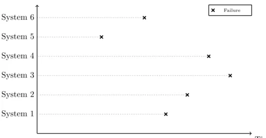
3.5.1 Complete data . . . 53
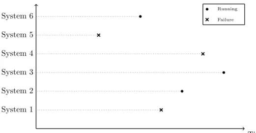
3.5.2 Right-censored data . . . 54
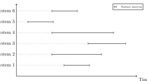
3.5.3 Interval-censored data . . . 54
3.5.4 Left-censored data . . . 54
3.6 Trend tests . . . 55
3.6.1 The reverse arrangement test . . . 55
3.6.2 The military handbook test . . . 56
3.7 Model parameter estimation methods . . . 58
3.7.1 The maximum likelihood method . . . 58
3.7.2 The least squares method . . . 59
3.7.3 The Bayesian parameter estimation method . . . 59
3.8 Acceleration models . . . 60
3.8.1 The Arrhenius model . . . 61
3.8.2 The Eyring model . . . 61
3.9 Chapter summary . . . 62
II Mathematical modelling framework 63 4 Mathematical model formulations 65 4.1 The GMS objective functions selected . . . 65
4.1.1 Minimising probability of unit failure . . . 65
4.1.2 Maximising expected energy production . . . 66
4.2 Model assumptions . . . 67
4.3 GMS models . . . 69
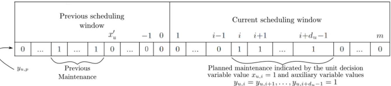
4.3.1 The model variables . . . 70
4.3.2 The objective functions . . . 70
4.3.3 The model constraints . . . 76
4.4 Chapter summary . . . 77
5 Model solution approaches 79 5.1 Linearisation of the model of §4.3 . . . 79
5.1.1 Piecewise linear function approximation . . . 79
5.1.2 Breakpoint selection during piecewise linear function approximation . . . 81
5.2 Exact model solution approach . . . 83
5.2.1 Motivation for the choice of optimisation platform . . . 83
5.2.2 CPLEX implementation . . . 84
5.3 Approximate model solution approach . . . 86
5.3.1 Motivation for the selected approximate solution methodology . . . 89
5.3.2 Simulated annealing implementation . . . 89
5.3.3 Experimental design . . . 95
III Academic benchmark results 99
6 Academic benchmark system data 101
6.1 The 21-unit system . . . 101
6.2 The 32-unit IEEE-RTS . . . 103
6.3 Chapter summary . . . 109
7 Minimising probability of unit failure 111 7.1 Exact solution results . . . 111
7.1.1 The 21-unit system . . . 111
7.1.2 The IEEE-RTS . . . 118
7.2 Approximate solution results . . . 124
7.2.1 The 21-unit system . . . 125
7.2.2 The IEEE-RTS . . . 138
7.3 Chapter summary . . . 153
8 Maximising expected energy production 157 8.1 Piecewise linear approximation results . . . 157
8.1.1 The 21-unit system . . . 157
8.1.2 The IEEE-RTS system . . . 167
8.2 Metaheuristic approximate solution approach . . . 177
8.2.1 The 21-unit system . . . 177
8.2.2 The IEEE-RTS . . . 190
8.3 Chapter summary . . . 204
IV Real-world model application 207 9 Case study data 209 9.1 Background . . . 209
9.2 Specifications . . . 209
9.3 Objective function extensions . . . 215
9.3.1 Minimising of probability of unit failure . . . 215
9.3.2 Maximising expected energy production . . . 220
9.4 Chapter summary . . . 224
10 Numerical results 227 10.1 Parameter optimisation experiments . . . 227
10.1.1 Minimising the probability of unit failure . . . 227
10.1.2 Maximising expected energy production . . . 228
10.2 Approximate solutions . . . 229
10.2.1 Minimising the probability of unit failure . . . 229
10.2.2 Maximising expected energy production . . . 234
10.3 Chapter summary . . . 239
11 Decision support framework 241 11.1 General considerations in decision support systems . . . 241
11.1.1 The database . . . 241
11.1.2 The graphical user interface . . . 242
11.1.3 The model base . . . 242
11.2 Detailed process description . . . 242
11.3 System development . . . 243 11.3.1 Data preparation . . . 243 11.3.2 System walk-thorough . . . 244 11.4 Chapter summary . . . 258 V Conclusion 259 12 Dissertation summary 261 12.1 Dissertation contents . . . 261
12.2 Appraisal of dissertation contributions . . . 264
13 Possible future work 269 13.1 Incorporating PGU generation capability variation . . . 269
13.2 Enforcing a maintenance interval constraint . . . 270
13.3 Failure frequency generalisation . . . 270
13.4 Incorporating PGUs with increasing failure rates . . . 270
13.5 The possibility of failures being dependent on one another . . . 271
13.6 Reliability accuracy improvement in the linear GMS model . . . 271
13.7 Adopting constraint programming as solution approach . . . 271
13.8 Adopting a multi-objective GMS paradigm . . . 272
A Eskom case study: Parameter optimisation experimental results 287 A.1 Minimising the probability of unit failure . . . 287 A.1.1 Initial acceptance ratio and soft constraint violation severity factor . . . . 287 A.1.2 Cooling parameter, reheating parameter and epoch parameter . . . 288 A.2 Maximising expected energy production . . . 289 A.2.1 Initial acceptance ratio and soft constraint violation severity factor . . . . 289 A.2.2 Cooling parameter, reheating parameter and epoch parameter . . . 290
List of Reserved Symbols
GMS model
Symbol Meaning
a Function value of a piecewise linear break point b Piecewise linear break point
Cu Rated capacity of PGU u
Cmax Rated capacity of largest PGU in the system
du Duration of planned maintenance to be performed on PGUu
E Expected energy produced
eu Earliest maintenance commencement date for PGU u
Fu Number of resources required for the maintenance of PGU u
fu,p,v Resource requirement parameter for maintenance during time period p if planned maintenance were to be scheduled to start during time period v on PGU u
I Maximum number of power generating units that may be scheduled for simul-taneous maintenance
J Set of PGUs which may not be in maintenance simultaneously
ku Time period during which maintenance of PGU u is scheduled to commence `u Latest maintenance commencement date of PGUu
Mp Number of available resources during planning period p m Number of planning periods within the scheduling window n Number of power generating units in the system
P Set of planning periods in the scheduling window
s Number of soft constraints
U Set of power generating units in the system
wu Number of maintenance intervals of PGU u within a given scheduling window Xu Random variable denoting the timing of the next failure of PGU u
x0u The time period during which PGUu entered into operation after its previous maintenance operation
xu,p GMS binary decision variable specifying the commencement date of mainte-nance of PGU u during time periodp
yu,p GMS binary auxiliary variable specifying that PGUuis in maintenance during time periodp
Earliest tarting time of the maintenance interval of a PGU
λu Failure rate of PGU u
τ Scheduling window
Indices
Symbol Meaning
p Planning period index
u Power generating unit index
v Scheduled planned maintenance commencement starting time
Simulated annealing
Symbol Meaning
Amin Minimum number of move acceptances
∆E Average deterioration in objective function values G Limiting values for the soft constraints
L Termination length of an epoch
T0 Initial temperature
α Cooling parameter
γ Soft constraint severity factor
ξ Reheating parameter
φ Multiplicative penalty function χ0 Initial acceptance ratio
List of Acronyms
Acronym Meaning
ACO Ant Colony Optimisation
B&B Branch-and-Bound
CDF Cumulative Distribution Function
CFR Constant Failure Rate
DFR Decreasing Failure Rate
DPSA Dynamic Programming Successive Approximation
DSS Decision Support System
EAF Energy Availability Factor
ED Economic Dispatch
EFS Energy Flow Simulator
ES Expert System
EUE Expected Unsupplied Energy
FOM Force Of Mortality
GA Genetic Algorithm
GENCO GENeration COmpany
GMS Generator Maintenance Scheduling GUI Graphical User Interface
HCI Human-Computer Interaction
HPP Homogeneous Poisson Process
IEEE Institute of Electrical and Electronics Engineers IFR Increasing Failure Rate
IP Integer Programming
IRP Integrated Resource Plan
ISO Independent System Operator
LOLE Loss Of Load Expectation LOLP Loss Of Load Probability
LP Linear Program
MHT Military Handbook Test
MILP Mixed Integer Linear Programming
MLE Maximum Likelihood Estimation
MTBF Mean Time Between Failures
MTTF Mean Time To Failure
NHPP Non-Homogeneous Poisson Process OCLF Other Capability Loss Factors PCLF Planned Capability Loss Factors PDF Probability Density Function
PGU Power Generating Unit
Acronym Meaning
PSO Particle Swarm Optimisation
RAT Reverse Arrangement Test
RT Reliability Theory
RTS Reliability Test System
SA Simulated Annealing
TS Tabu Search
UC Unit Commitment
List of Figures
1.1 Energy production and consumption in South Africa . . . 2
2.1 Benders’ decomposition flow diagram . . . 29
3.1 The well-known bathtub curve . . . 42
3.2 A graphical representation of complete data . . . 53
3.3 A graphical representation of right censored data . . . 54
3.4 A graphical representation of interval censored data . . . 55
3.5 A graphical representation of left censored data . . . 55
3.6 A graphical representation of Qend . . . 57
3.7 Military handbook test outcomes . . . 57
3.8 Laplace trend test outcomes . . . 58
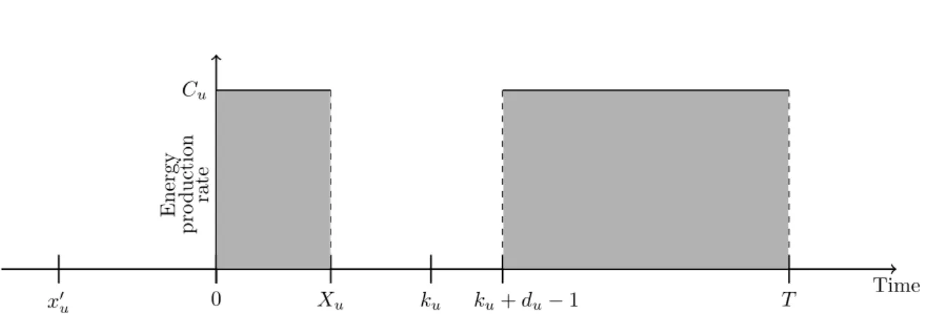
4.1 A graphical representation of variables and parameters . . . 70
4.2 The reliability of a PGU . . . 71
4.3 The expected energy produced in three different cases . . . 75
5.1 A piecewise linear function . . . 80
5.2 Parameters and variables in CPLEX. . . 85
5.3 Parameter inputs required for implementation of the GMS models . . . 86
5.4 Objective function and constraint implementations in CPLEX . . . 87
5.5 An alternative objective function implementation in CPLEX . . . 88
5.6 Ejection chain neighbourhood move operator example . . . 93
6.1 The true value and piecewise linear approximation (21-unit system) . . . 104
6.2 IEEE-RTS demand data . . . 106
6.3 The true value and piecewise linear approximation (IEEE-RTS) . . . 108
7.1 An optimal maintenance schedule for the 21-unit system (linear) . . . 112 7.2 The manpower required by and system capacity of the 21-unit system (optimal) 113
7.3 Probability of failure for each PGU of the 21-unit system . . . 114 7.4 Comparison between two maintenance schedules for the 21-unit system (linear) . 116 7.5 An optimal maintenance schedule for the IEEE-RTS (linear) . . . 119 7.6 The manpower required by and system capacity of the IEEE-RTS (optimal) . . . 120 7.7 Comparison between two maintenance schedules for the IEEE-RTS (linear) . . . 122 7.8 The manpower required by and system capacity of the IEEE-RTS (linear, SSR) . 123 7.9 Linear model optimality gap box plots for the 21-unit system (Phase 1) . . . 127 7.10 Linear model computation time for the 21-unit system (Phase 1) . . . 128 7.11 The 21-unit system infeasible incumbents of the linear model (Phase 1) . . . 129 7.12 Linear model optimality gap box plots for the 21-unit system (Phase 2) . . . 133 7.13 Linear model computation time for the 21-unit system (Phase 2) . . . 134 7.14 The 21-unit system infeasible incumbents of the linear model (Phase 2) . . . 134 7.15 The incumbent returned by the SA algorithm for the 21-unit system (linear) . . 136 7.16 The manpower required by and system capacity of the 21-unit system (incumbent)137 7.17 Maintenance schedule comparison for the 21-unit system (linear) . . . 138 7.18 The manpower required by and system capacity of the 21-unit system (linear) . . 139 7.19 Linear model optimality gap box plots for the IEEE-RTS (Phase 1) . . . 141 7.20 Linear model computation time for the IEEE-RTS (Phase 1) . . . 142 7.21 The IEEE-RTS infeasible incumbents of the linear model (Phase 1) . . . 144 7.22 Linear model optimality gap box plots for the IEEE-RTS (Phase 2) . . . 147 7.23 Linear model computation time for the IEEE-RTS (Phase 2) . . . 148 7.24 The IEEE-RTS infeasible incumbents of the linear model (Phase 2) . . . 148 7.25 The incumbent returned by the SA algorithm for the IEEE-RTS (linear) . . . 151 7.26 The manpower required by and system capacity of the IEEE-RTS (incumbent) . 152 7.27 Maintenance schedule comparison for the IEEE-RTS (exact) . . . 153 7.28 The manpower required by and system capacity of the IEEE-RTS (exact) . . . . 154 8.1 An optimal maintenance schedule for the 21-unit system (nonlinear) . . . 158 8.2 The manpower required by and system capacity of the 21-unit system (nonlinear) 159 8.3 Expected energy production for each PGU of the 21-unit system . . . 160 8.4 Comparison between two maintenance schedules for the 21-unit system (SSR) . . 162 8.5 Comparison between two maintenance schedules for the 21-unit system (probability)164 8.6 An optimal maintenance schedule for the IEEE-RTS (nonlinear) . . . 168 8.7 The manpower required by and system capacity of the IEEE-RTS (nonlinear) . . 169 8.8 Comparison between two maintenance schedules for the IEEE-RTS (SSR) . . . . 170 8.9 The manpower required by and system capacity of the IEEE-RTS solution (SSR) 171
8.10 Comparison between two maintenance schedules for the IEEE-RTS (probability) 173 8.11 The manpower required by and system capacity of the IEEE-RTS (probability) . 174 8.12 Nonlinear model optimality gap box plots for the 21-unit system (Phase 1) . . . 179 8.13 Nonlinear model computation time for the 21-unit system (Phase 1) . . . 180 8.14 The 21-unit system infeasible incumbents of the nonlinear model (Phase 1) . . . 181 8.15 Nonlinear model optimality gap box plots for the 21-unit system (Phase 2) . . . 184 8.16 Nonlinear model computation time for the 21-unit system (Phase 2) . . . 186 8.17 The 21-unit system infeasible incumbents of the nonlinear model (Phase 2) . . . 186 8.18 The incumbent returned by the SA algorithm for the 21-unit system (nonlinear) 188 8.19 The manpower required by and system capacity of the 21-unit system (incumbent)189 8.20 Maintenance schedule comparison for the 21-unit system (nonlinear) . . . 190 8.21 The manpower required by and system capacity of the 21-unit system (comparison)191 8.22 Nonlinear model optimality gap box plots for the IEEE-RTS (Phase 1) . . . 193 8.23 Nonlinear model computation time for the IEEE-RTS (Phase 1) . . . 194 8.24 The IEEE-RTS infeasible incumbents of the nonlinear model (Phase 1) . . . 195 8.25 Nonlinear model optimality gap box plots for the IEEE-RTS (Phase 2) . . . 198 8.26 Nonlinear model computation time for the IEEE-RTS (Phase 2) . . . 200 8.27 The IEEE-RTS infeasible incumbents of the nonlinear model (Phase 2) . . . 201 8.28 The incumbent returned by the SA algorithm for the IEEE-RTS (nonlinear) . . . 203 8.29 The manpower required by and system capacity of the IEEE-RTS (incumbent) . 204 8.30 Maintenance schedule comparison for the IEEE-RTS (nonlinear) . . . 205 8.31 The manpower required by and system capacity of the IEEE-RTS (comparison) . 206 9.1 157-unit Eskom case study demand data . . . 213 9.2 The reliability of a PGU requiring multiple maintenance procedures . . . 221 9.3 Failure in Case I . . . 222 9.4 Failure in Case II . . . 223 9.5 Failure in Case III . . . 223 9.6 Expected energy produced by PGU 105 . . . 225 10.1 Incumbent returned by the linear SA model for the case study (capacity) . . . . 231 10.2 Incumbent returned by the linear SA model for the case study (failure rate) . . . 232 10.3 System capacity for the 157-unit Eskom case study for the linear model . . . 233 10.4 Incumbent returned by the nonlinear SA model for the case study (capacity) . . 236 10.5 Incumbent returned by the nonlinear SA model for the case study (failure rate) . 237 10.6 System capacity for the 157-unit Eskom case study for the nonlinear model . . . 238
11.1 Graphical DDS overview . . . 243 11.2 Demand specification format . . . 244 11.3 PGU specifications format . . . 245 11.4 Home scree of the DSS . . . 246 11.5 File input GUI . . . 247 11.6 Summary of system tab (eight percent safety margin) . . . 248 11.7 Summary of system tab (fifteen percent safety margin) . . . 249 11.8 PGU specifications tab . . . 250 11.9 Demand specifications tab . . . 251 11.10 Algorithm specifications window . . . 252 11.11 Algorithm overview tab . . . 253 11.12 Maintenance schedule tab . . . 254 11.13 Maintenance starting times . . . 255 11.14 Available capacity tab . . . 256 11.15 Required manpower tab . . . 257
List of Tables
1.1 Plant mix of Eskom . . . 2 3.1 Reverse arrangement test critical values . . . 56 5.1 Triangular matrix containing the SSR . . . 82 5.2 Parameter values of the parameter experiment for the 21-unit system (Phase 1) . 95 5.3 Parameter values of the parameter experiment for the 21-unit system (Phase 2) . 95 6.1 The 21-unit test system specifications . . . 102 6.2 Time elapsed since previous PGU maintenance for the 21-unit system . . . 102 6.3 Piecewise linearisation breakpoints for the 21-unit system . . . 103 6.4 The IEEE-RTS specifications . . . 105 6.5 Exclusion sets for IEEE-RTS . . . 105 6.6 The IEEE-RTS demand per week . . . 106 6.7 Time elapsed since previous PGU maintenance for the IEEE-RTS . . . 107 6.8 Piecewise linearisation breakpoints for the IEEE-RTS . . . 107 7.1 Objective function value comparison for the 21-unit system (linear) . . . 115 7.2 Statistics pertaining to the optimal solutions of the 21-unit system (linear) . . . 117 7.3 Groups of PGUs for the IEEE-RTS with similar specifications . . . 121 7.4 Objective function value comparison for the IEEE-RTS (linear) . . . 122 7.5 Statistics pertaining to the optimal solutions of the IEEE-RTS (linear) . . . 124 7.6 Linear model optimality gaps for the 21-unit system (Phase 1) . . . 125 7.7 Linear model computation times for the 21-unit system (Phase 1) . . . 126 7.8 The 21-unit system infeasible incumbents of the linear model (Phase 1) . . . 126 7.9 The 21-unit system final parameter values of linear model (Phase 1) . . . 130 7.10 Linear model optimality gaps for the 21-unit system (Phase 2) . . . 130 7.11 Linear model computation times for the 21-unit system (Phase 2) . . . 131 7.12 The 21-unit system infeasible incumbents of the linear model (Phase 2) . . . 131
7.13 The parameters finally selected for the 21-unit system (linear) . . . 135 7.14 Linear model optimality gaps for the IEEE-RTS (Phase 1) . . . 140 7.15 Linear model computation times for the IEEE-RTS (Phase 1) . . . 140 7.16 The IEEE-RTS infeasible incumbents of the linear model (Phase 1) . . . 140 7.17 The IEEE-RTS final parameter values of the linear model (Phase 1) . . . 143 7.18 Linear model optimality gaps for the IEEE-RTS (Phase 2) . . . 145 7.19 Linear model computation times for the IEEE-RTS (Phase 2) . . . 145 7.20 The IEEE-RTS infeasible incumbents of the linear model (Phase 2) . . . 146 7.21 The parameters finally selected for the IEEE-RTS (linear) . . . 150 8.1 Objective function value comparison for the 21-unit system (SSR) . . . 161 8.2 Objective function value comparison for the 21-unit system (probability) . . . 163 8.3 Statistics pertaining to the optimal solutions of the 21-unit system (nonlinear) . 166 8.4 Objective function value comparison for the IEEE-RTS (SSR) . . . 172 8.5 Objective function value comparison for the IEEE-RTS (probability) . . . 175 8.6 Statistics pertaining to the optimal solutions of the IEEE-RTS (nonlinear) . . . . 176 8.7 Nonlinear model optimality gaps for the 21-unit system (Phase 1) . . . 178 8.8 Nonlinear model computation times for the 21-unit system (Phase 1) . . . 178 8.9 The 21-unit system infeasible incumbents of the nonlinear model (Phase 1) . . . 178 8.10 The 21-unit system final parameter values of the nonlinear model (Phase 1) . . . 182 8.11 Nonlinear model optimality gaps for the 21-unit system (Phase 2) . . . 183 8.12 Nonlinear model computation times for the 21-unit system (Phase 2) . . . 183 8.13 The 21-unit system infeasible incumbents of the nonlinear model (Phase 2) . . . 183 8.14 The parameters finally selected for the 21-unit system (nonlinear) . . . 187 8.15 Nonlinear model optimality gaps for the IEEE-RTS (Phase 1) . . . 192 8.16 Nonlinear model computation times for the IEEE-RTS (Phase 1) . . . 192 8.17 The IEEE-RTS infeasible incumbents of the nonlinear model (Phase 1) . . . 192 8.18 The IEEE-RTS final parameter values of the nonlinear model (Phase 1) . . . 196 8.19 Nonlinear model optimality gaps for the IEEE-RTS (Phase 2) . . . 197 8.20 Nonlinear model computation times for the IEEE-RTS (Phase 2) . . . 197 8.21 The IEEE-RTS infeasible incumbents of the nonlinear model (Phase 2) . . . 197 8.22 The parameters finally selected for the IEEE-RTS (nonlinear) . . . 201 9.1 Description of the PGUs in the Eskom case study . . . 210 9.2 The actual PGU specifications for the 157-unit Eskom case study . . . 210 9.3 Demand required per day for the 157-unit Eskom case study . . . 214
9.4 The 157-unit Eskom case study specifications . . . 216 10.1 Parameters finally selected for the 157-unit Eskom case study (linear model) . . 228 10.2 Parameters finally selected for the 157-unit Eskom case study (nonlinear model) 229 10.3 Decision variable values for the 157-unit Eskom case study (linear model) . . . . 230 10.4 Decision variable values for the 157-unit Eskom case study (nonlinear model) . . 235 A.1 Objective function values in the parameter experiment (Phase 1, linear model) . 287 A.2 Computation times of the parameter experiment (Phase 1, linear model) . . . 288 A.3 The infeasible incumbents of the parameter experiment (Phase 1, linear model) . 288 A.4 Objective function values in the parameter experiment (Phase 2, linear model) . 288 A.5 Computation times of the parameter experiment (Phase 2, linear model) . . . 289 A.6 The infeasible incumbents of the parameter experiment (Phase 2, linear model) . 289 A.7 Objective function values in parameter experiment (Phase 1, nonlinear model) . 290 A.8 Computation times of the parameter experiment (Phase 1, nonlinear model) . . . 290 A.9 The infeasible incumbents of parameter experiment (Phase 1, nonlinear model) . 290 A.10 Objective function values in parameter experiment (Phase 2, nonlinear model) . 291 A.11 Computation times of the parameter experiment (Phase 2, nonlinear model) . . . 291 A.12 The infeasible incumbents of parameter experiment (Phase 2, nonlinear model) . 291
List of Algorithms
5.1 Determining an SA initial temperature . . . 90 5.2 Ejection chain SA move operator . . . 94 5.3 GMS simulated annealing . . . 96
CHAPTER 1
Introduction
Contents
1.1 Background . . . 1
1.2 Informal problem description . . . 4
1.3 Dissertation scope and objectives . . . 5
1.4 Dissertation organisation . . . 6
1.1 Background
The sustainability of modern society is heavily dependent on a secure and accessible supply of energy [63]. Power utilities have become one of the most crucial resources in any nation’s economy and therefore the operations planning of these utilities is of utmost importance [104]. Such operations planning is particularly challenging in the context of developing countries, because the electricity demands in these countries typically increase rapidly due to fast evolving economies [12]. Not only are electricity utilities pressured to meet the ever-changing demands in such countries, they are also pressured to remain current in respect of global energy policies that are currently pushing for “greener energy.” This places additional strain on the capital reserves of developing countries, because cleaner energy sources typically still come at a much greater cost than the more traditional methods of electricity generation [63].
In South Africa, which is classified as a developing country [119], Eskom is the sole power utility and was established in 1923 as the Electricity Supply Commission. It was then converted into a public, limited-liability company in 2002 that is wholly owned by the government of South Africa [75]. Today Eskom is recognised as one of the top twenty power utilities in the world, based on generation capacity, with a net maximum self-generated capacity of approximately 44 184 MW. Eskom supplies more than 45% of the electricity consumed in Africa and supplies approximately 96% of South Africa’s electricity [76]. The production and consumption of power in South Africa over the past 17 years are presented in Figures 1.1(a) and 1.1(b), respectively. Although almost 86% of the total installed generation capacity in South Africa is coal-fire based, alternative forms of renewable energy sources are constantly researched by the utility. The combination of the various technologies used to generate electricity is called the plant mix which, for Eskom, is shown in Table 1.1 [76]. As may be seen in the table, Eskom utilises six technologies in its electricity generation operations. Power stations are either classified as base load stations or as peak demand stations. Base load stations are stations that operate every day
2000 2001 2002 2003 2004 2005 2006 2007 2008 2009 2010 2011 2012 2013 2014 2015 2016 180 200 220 240 260 280 Year Pro duction (TWh)
(a)The power production in South Africa over the past 17 years [72]
2000 2001 2002 2003 2004 2005 2006 2007 2008 2009 2010 2011 2012 2013 2014 2015 2016 140 160 180 200 220 Year Consumption (TWh)
(b)The power consumption in South Africa over the past 17 years [72]
Figure 1.1: The energy production and consumption of South Africa over the past 17 years.
of the year, whereas peak demand stations only operate when the demand exceeds the supply capability of the base load stations.
Coal-fired power stations use coal as their primary fuel source. These stations are the work-horses of the South African power utility and are required to operate 24 hours a day in order to meet the country’s energy demand, with the exception of being offline when scheduled for planned maintenance or when failures occur.
Table 1.1: The plant mix of Eskom’s electricity generating technologies as on 4 October 2017 [76].
Type # Power Plants Type Plant mix
Coal-fired stations 13 Base Load 85.43%
Nuclear stations 1 Base Load 4.32%
Hydro stations 2 Peak Demand 1.36%
Pumped storage schemes 2 Peak Demand 3.17%
Gas fired stations 4 Peak Demand 5.49%
Africa’s first and only nuclear power station, Koeberg, has a total installed capacity of 1 910 MW and is located in Melkbosstrand within the Western Cape [76].
The third generation technology that Eskom employs is hydro energy power stations. These peak demand stations capture the energy of moving water from dams or in rivers and convert the kinetic energy to electrical energy. The two hydro power stations of Eskom are located in the Gariep dam near Norvalspont and in the Vanderkloof dam near Petrusville, respectively [76]. Another technology which also uses the kinetic energy of moving water is a pump storage scheme. This type of facility is also classified as a peak demand station. These stations work on the same principle as hydro power stations, but reuse the water that was used to generate electricity by pumping it back to a storage reservoir up-river during off-peak times to be reused during subsequent peak demand times [77].
The plant mix also contains four gas turbine power stations which have very quick start-up times, but also very high operating costs due to their use of kerosene and diesel as primary fuel sources. These stations are therefore only used during peak demand periods and during emergencies.
Eskom has additionally invested in two wind farms, one of which has already been in operation since 2002 and another which came into full operation early in 2015. The first wind farm consists of only three wind turbines with an installed capacity of merely 3 MW. The second wind farm, which is situated near Vredendal in the Western Cape, consists of 46 wind turbines with a combined installed capacity of 100 MW [76].
During 2015, the electricity system of South Africa was severely challenged and experienced a tightly constrained demand/supply balance, which put the power system at risk in respect of both its adequacy and reliability. This situation may be attributed to the fact that during the 1980s there was an excess supply of electricity due to an electricity generation expansion programme launched by Eskom during the late 1970s. As a result, little or no investments were made in the generation expansion of Eskom during the 1990s and early 2000s [125].
Also contributing to the highly constrained South African energy system, was the higher than expected demand since 2008. This caused nationwide blackouts and since then strain on the system has only recently decreased. Following this, Eskom introduced “load shedding” to the nation. Load shedding involves a series of planned rolling blackouts that follows a rotating schedule. It is used to decrease the demand during periods when Eskom cannot meet the required demand and the short supply threatens the integrity of the nation’s electricity grid [103].
Another reason for the situation that Eskom found itself in during 2015, is inadequate mainte-nance planning. It was recognised at the quarterlyState of the System briefing held on January 15th, 2015 that a major reason for the previous South African energy situation is that Eskom had not performed the necessary maintenance on thepower generating units (PGUs) of its power plants [89]. The required maintenance downtimes of PGUs had been postponed on a continual basis due to the high energy demand experienced. Although Eskom had a specific maintenance philosophy in place, it had not remained completely faithful to this philosophy and was therefore faced with massive challenges [89].
A power utility’s ability to satisfy energy demand can be influenced significantly by unexpected breakdowns of PGUs. In most cases, such unexpected failures are also much more expensive to repair than taking planned preventative maintenance action. Maintenance of ageing PGUs is, however, often neglected due to high energy demand and low system capacity, as seen in the case of Eskom. The typical objectives pursued in the design of PGU maintenance schedules do not take these difficulties into account. Two new scheduling criteria are therefore proposed in
this dissertation in order to explore to what extent generator maintenance scheduling (GMS) optimisation can contribute to the reliability of a power utility’s operations.
1.2 Informal problem description
An electricity utility, such as Eskom, typically strives to maintain a reserve margin for generation capacity of 15%. During 2015, the capacity required by the South African grid exceeded supply by approximately 7.5%. This meant that the reserve margin for generation capacity dropped to approximately 7.5%, which is half of the desired reserve margin [49]. This low percentage can cause blackouts when sudden fluctuations in electricity demand are experienced and is therefore a serious problem for any power utility. In the case of Eskom, this drop in reserve margin is partially attributable to the utility not remaining entirely faithful to its own maintenance philos-ophy pre 2014/2015, as mentioned in the previous section. After falling behind on maintaining the PGUs of power stations, Eskom was faced with a number of unexpected downtimes at power stations and was therefore often unable to achieve the desired reserve margin, resulting in the implementation of load shedding.
Currently, the capability of providing maintenance scheduling recommendations by determining a power utility’s expected capacity to satisfy energy demand is not specifically incorporated in the GMS designs in the literature and therefore research is conducted in this dissertation to enable such a capability. Maintenance schedules may be determined by solving incarnations of the celebrated GMS problem, which aims to find a good planned maintenance schedule for the PGUs in a power system in such a way that energy demand is satisfied effectively and efficiently. Recent and current developments in the GMS literature do not, however, take into account the reliability of the PGUs in a power system when scheduling maintenance. In a power system that has been in operation for a considerable number of years, such as in the case of Eskom, the reliability of the PGUs in the system may be compromised. Hence there exists a need for the capability of scheduling planned preventative maintenance procedures based on the probability that a PGU will fail, which is very dependent on the PGU’s age. The expected energy produced by a system over a given scheduling window may also be determined based on the probability of PGU failure, which may be employed as an alternative scheduling criterion.
Two novel scheduling criteria are consequently proposed as objective functions to the GMS problem in this dissertation, the first of which takes into account the probability of PGUs fail-ing. This function is proposed so as to be able to quantify an entire power system’s reliability in terms of PGU failures. Another novel scheduling criterion is also proposed as an alternative objective function for the GMS problem which aims quantify an entire power system’s reliability in terms of the expected energy production over a given scheduling window, taking into account the probability of PGU failure. Both these scheduling criteria are included in the constrained framework of standard GMS models in order to analyse the effectiveness of scheduling planned maintenance according to such criteria. The proposed scheduling criteria are expected to facili-tate reduction of the chance of load shedding having to be implemented by scheduling planned maintenance in pursuit of avoiding PGU failures — events that may cause sudden drops in available energy capacity.
The aforementioned two GMS model considerations may then be employed to provide good maintenance schedules for power systems and may eventually be incorporated into a decision support framework in aid of power utilities with respect to daily GMS decision making.
1.3 Dissertation scope and objectives
The following twelve objectives are pursued in this dissertation: I Toconduct a thorough survey of the literature related to:
(a) the elements typically taken into consideration in GMS decisions in general, (b) the derivation of model formulations for the GMS problem,
(c) appropriate solution approaches designed for instances of the GMS problem, (d) the constituent models and methodologies of reliability theory in general,
(e) trend tests related to identifying repairable and non-repairable systems,
(f) lifetime models related to repairable and non-repairable systems in reliability theory, (g) estimation methods for repairable and non-repairable lifetime model parameters, (h) acceleration models for failure analysis.
II Toestablish a mathematical modelling framework capable of quantifying the reliability of an electric power system in terms of:
(a) power generating unit failure, and (b) expected energy production
over a specified maintenance planning horizon, which may be used in optimisation ap-proaches toward solving instances of the GMS problem. The framework should include the techniques researched in pursuit of Objectives I(c)–(h).
III To formulate novel single-objective combinatorial optimisation models for the GMS prob-lem in the context of maximising power system reliability. The models should be based on the modelling frameworks of Objectives II(a) and II(b).
IV To design a generic decision support system (DSS) capable of providing good planned maintenance schedules for the PGUs in a power system aimed at maximising the system’s reliability (by either minimising probability of unit failure or maximising expected energy production). The DSS should draw on the techniques researched in pursuit of Objective I and should contain the models formulated in pursuit of Objective III.
V Toimplement a concept demonstrator of the DSS of Objective IV in a suitable application software platform. The concept demonstrator should be able to take as input the demand and system specifications of a user-specified power generating system, as well as related user-specified parameters for the GMS problem, and it should produce as output a high-quality maintenance schedule for the PGUs in the system.
VI Toverifyandvalidatethe system designed in pursuit of Objective IV according to generally accepted modelling guidelines. An exact solution approach should be employed in the context of small problem instances and an approximate solution approach in the context of larger problem instances to aid in the verification and validation process.
VII To apply the system designed in pursuit of Objective IV in special case studies involving the celebrated 21-unit GMS test system [54] and the IEEE-RTS [188] benchmark GMS system in the literature.
VIII To evaluate the effectiveness of the system’s outputs in the context of the case studies of Objective VII.
IX To establish a real-world case study which is based on the power system of the national power utility of South Africa, Eskom.
X To apply the system designed in pursuit of Objective IV to the real-world case study of Objective IX.
XI Toevaluate the effectiveness of the system’s outputs in the context of the real-world case study of Objective IX.
XII To recommend sensible follow-up work related to the work in this dissertation which may be pursued in the future.
The scope of this dissertation is such that other related energy problems, such as the unit commitment problem [186, 192, 207], the economic dispatch problem [16, 82] or the transmission scheduling problem [67, 68, 152], are not considered. The research is also limited by only taking into account the risk associated with unexpected failures of PGUs and not the risk associated with any lost opportunity cost as a result of planned maintenance being performed.
1.4 Dissertation organisation
This dissertation comprises twelve further chapters which are organised into five parts, as well as two appendices. In§2, which is the first chapter in a two-chapter part dedicated to a review of the literature, the reader is introduced to the GMS problem and a number of considerations gener-ally addressed when formulating GMS models, including energy problems that are related to the GMS problem. A review of the literature on GMS model formulations is presented next, includ-ing mathematical programminclud-ing formulations containinclud-ing popular objective functions as well as constraint sets typically included. This is followed by a thorough review of solution approaches that have been adopted in the literature to solve instances of the GMS problem, including mathematical programming techniques, expert systems, fuzzy logic approaches, heuristics and metaheuristics. A separate, more detailed review section is dedicated to the method ofsimulated annealing (SA), as this method is applied as the approximate model solution methodology in this dissertation.
The second chapter in Part I of this dissertation,§3, is devoted to reliability theory. The reader is introduced to various fundamental concepts in the theory of reliability. This is followed by a review of the basic mathematical notations required to represent various ideas within reliability theory. Two types of systems are typically considered in reliability theory, namely non-repairable systems and repairable systems, both of which are described in §3, along with popular distribution models used in each of these cases. The section is followed by a description of typical failure data employed to approximate failure models for these systems. A section on trend tests is also included. These tests may be employed to determine whether or not there exists a trend in the failure times of a data set. The next section is devoted to the estimation of failure model parameters, including the maximum likelihood method, the least squares method and the Bayesian parameter estimation method. In the final section of the chapter, the reader is introduced to the notation of acceleration models which describe ways of modelling systems that operate under high stress.
Part II of this dissertation also contains two chapters and is concerned with establishing a mathematical framework two newly the proposed GMS models. In §4, mathematical models are
formulated for two incarnations of the GMS problem considered in this dissertation. The first section of the chapter provides a motivation for the design the two newly proposed objective functions as scheduling criteria, one of which is linear and one which is nonlinear. This is followed by a discussion on the assumptions made in order to facilitate derivation of both mathematical models. The next section contains a description of the actual GMS models adopted in this dissertation. The section includes a detailed derivation of the two proposed objective functions and a mathematical representation of the model constraints. The constraint sets included in the GMS models are energy demand satisfaction constraints, maintenance window constraints, maintenance resource constraints and maintenance exclusion constraints.
Two methodologies are adopted in this dissertation to solve the GMS models of §4. These methodologies are described in some detail in §5, which is the second chapter in Part II. One of these methodologies is an exact solution approach and the other is an approximate solution approach. Both methodologies are particularly tailored to instances of the GMS models pro-posed in §4. The fist section of the chapter contains a description of a method which may be employed to linearise the nonlinear GMS model proposed in §4.3. A piecewise linear approxi-mation method is proposed in which the optimal positions for breakpoints are determined by employing dynamic programming. The second section of the chapter contains a description of the exact solution approach adopted, a motivation for the choice of optimisation platform (CPLEX) and a description of the implementations within this platform of both the linear and nonlinear models. The third section contains a general introduction to the approximate solution approach, namely the method of SA. The section also includes a motivation for the choice of this solution methodology as well as a detailed discussion on the implementation of the method of SA. The discussion on the implementation of the technique covers a method for determining initial solutions and the initial temperature for the algorithm, the cooling and reheating sched-ules employed, the constraint handling technique implemented, the epoch management protocol adopted, the neighbourhood move operator selected and the termination criteria enforced. The third part of this dissertation contains three chapters and is dedicated to a decumentation of and discussion on the results returned by the various solution methods for the proposed GMS models with respect to two academic benchmark systems from the literature. The two benchmark systems considered in order to test the effectiveness of the newly proposed GMS objectives and the two solution approaches are described in the first chapter of Part III, §6. This description includes reference to the input data and parameters pertaining to these two systems. These two systems are a 21-unit test system and the celebrated 32-unit IEEE-RTS. The more basic 21-unit test system is presented in the first section of the chapter, contains 21 PGUs and exhibits a constant peak demand over a scheduling horizon of 52 one-week planning periods. The second section contains a description of the larger IEEE-RTS, which contains 32 PGUs and exhibits a varying peak demand, attributed to seasonal demand requirements. In the second chapter of Part III, the seventh chapter of the dissertation, the numerical results obtained when employing the minimisation of the probability of unit failure scheduling criterion are presented. The first section of the chapter contains a presentation of the results returned by the exact solution approach adopted for both the 21-unit test system and the IEEE-RTS. The results of this section represent optimal maintenance schedules in respect of the newly proposed GMS objective function as well as an analysis of the manpower required and available system capacity associated with these solutions. The optimal solutions obtained are also compared to solutions from the literature for an alternative GMS model involving the well-known minimisa-tion of the sum of squared reserve margins as scheduling criterion. Sensitivity analyses are also performed in order to analyse the feasibility of the exact solution approach for small systems such as the 21-unit test system and the IEEE-RTS. In the second section of the chapter, the
approximate solution approach results are presented for both the 21-unit test system and the IEEE-RTS. In this section, the results of the experimental design followed to determine the best combination of parameters for use in the method of SA are presented for both benchmark systems. These parameters include an initial SA acceptance ratio, a constraint violation sever-ity factor, a cooling parameter, a reheating parameter and an epoch termination parameter. The presentation of the results obtained from the parameter optimisation experiment include comparisons between the different combinations of parameters in order to obtain the best com-bination. Thereafter, the section also contains the solutions obtained when solving both the 21-unit test system and the IEEE-RTS by the method of SA as well as comparisons of the solutions thus obtained with the corresponding exact solutions.
The final chapter of Part III, which is the eighth chapter in the dissertation, follows the same structure as that of §7, but the numerical results obtained by employing the maximisation of the expected energy production scheduling criterion are presented instead. The first section of the chapter contains a presentation of the results returned by the exact solution approach after employing the piecewise linearisation approach described in §5. This presentation includes results for both the 21-unit test system and the IEEE-RTS. An optimal maintenance sched-ule for the piecewise linear approximation is provided in respect of the newly proposed GMS objective function as is an analysis of the manpower required and available system capacity associated with these solutions. The optimal solutions obtained are also compared with solu-tions from the literature for a GMS model involving the well-known minimisation of the sum of squared reserve margins as scheduling criterion. Sensitivity analyses are also performed in order to analyse the feasibility of the exact solution approach for small systems, such as the 21-unit test system and the IEEE-RTS, as was performed for the minimisation of the probability of unit failure scheduling criterion. In the second section of this chapter, the approximate solution approach results obtained when employing the maximisation of the expected energy production scheduling criterion are presented for both the 21-unit test system and the IEEE-RTS. In this section, the results of the experimental design followed to determine the best combination of parameters for use in the method of SA are presented for both benchmark systems are pre-sented. The same parameter ranges are considered for the maximisation of the expected energy production scheduling criterion as was the case for the minimisation of the probability of unit failure scheduling criterion in order to obtain the best combination. Thereafter, solutions are presented for the 21-unit test system and the IEEE-RTS by applying the SA solution approach upon adoption of the best parameter value combination returned by the experimental design. The section closes with comparisons of the solutions thus obtained with the exact solutions. The penultimate part of the dissertation, Part IV, is aimed at facilitating application of the proposed GMS to a real-world scenario. This part consists of three chapters, the first of which contains a description of the real-world case study considered in some detail in this dissertation. The case study is called the 157-unit Eskom case study and is based on the energy grid of the national power utility in South Africa. The first section of §9 provides some background on the case study and this is followed by detailed specifications of the power system. In the final section of the chapter, some extensions are proposed to the linear and nonlinear GMS objective functions of §4.3 in order to accommodate the situation where PGUs have to be scheduled for maintenance multiple times within a given scheduling window.
The results obtained by employing the approximate solution approach adopted in this disserta-tion to the real-world case study of §9, are presented and analysed in §10, the second chapter in Part IV, within the context of both the linear and nonlinear GMS models proposed in §4. The first section of the chapter is dedicated to the results obtained by employing the minimisa-tion of the probability of unit failure scheduling criterion as well as an analysis of the available
system capacity associated with this solution. The second section follows the same structure, but is dedicated to the results obtained by employing the maximisation of the expected energy production GMS objective function.
Part IV finally closes in §11 with the proposal of a computerised DSS, designed by the author, which is aimed at facilitating effective GMS decision making. In the first section of the chapter, some general consideration is given to typical DSS development. This includes a description of the three main components of a typical DSS and is followed by a detailed process description of the GMS DSS proposed. Finally, the system is described in a comprehensive system walk-through fashion aimed at informing potential users how to utilise the DSS to its full potential. The final part of this dissertation, Part V, contains two final chapters. The penultimate chapter of the dissertation, §12, contains a summary of the research performed, as documented in this dissertation, as well as an appraisal of the contributions made within this dissertation.
The final chapter, §13, contains an elaboration on seven suggestions for future work in the field of GMS that may follow naturally on the research performed in this dissertation.
Part I
Literature review
CHAPTER 2
Generator maintenance scheduling
Contents
2.1 Model considerations . . . 13
2.2 GMS model formulations in literature . . . 17
2.3 GMS model solution approaches . . . 26
2.4 The method of simulated annealing . . . 36
2.5 Chapter summary . . . 39
This chapter contains a literature review on thegenerator maintenance scheduling (GMS) prob-lem. Various generic GMS modelling considerations are considered in §2.1. In §2.2, a brief overview is given of the most commonly adopted GMS model formulations. This is followed in §2.4 by a brief description of the celebrated method of simulated annealing as applicable to GMS problem instances. Other model solution approaches are also described in §2.3, including various mathematical programming techniques, as well as the use of expert systems, fuzzy logic, heuristics and metaheuristics other than simulated annealing.
2.1 Model considerations
Scheduling the maintenance of the PGUs of power utilities is of utmost importance in energy system design, planning and operations management [188]. The planning involved the scheduling of such units for maintenance increases in complexity as the number of PGUs increases and as the reserve margin of the system decreases (i.e. the demand increases) [188]. GMS typically involves scheduling PGUs for preventative maintenance over a certain scheduling window in pursuit of a set of objectives and subject to a number of operational and system constraints in order to ensure schedule feasibility. Preventative maintenance performed on PGUs is directly related to a power utility’s ability to supply the required energy demand [135]. Three main goals are typically pursued in the design of good maintenance schedules for the PGUs of a power utility [5], namely:
(a) to increase the economic benefits and the reliability of the entire electrical system, (b) to extend the lifetime of the individual PGUs, and
(c) to avoid the installation of new PGUs. 13
Before the GMS problem may be formulated mathematically, four planning considerations have to be taken into account, namely the length of the scheduling window, the scheduling resolution, the particular constraints included in the model and the scheduling objectives to be pursued.
2.1.1 The scheduling window
The GMS problem is formulated over a so-called scheduling window which is an interval of planning periods over which the user, typically a power utility, aims to schedule preventative maintenance of PGUs into the future. The scheduling window of the GMS problem typically varies from a number of weeks to a number of years in the literature, although one year is the most common scheduling window adopted [5, 134], since PGUs are generally serviced on an annual basis [137].
Another reason why a one-year scheduling window is such a popular choice may be that the load demand is typically forecast by power utilities over a period of some multiple of years, because power utilities typically attempt to include all four seasons in their forecast planning [188]. There are, however, cases in the literature where the length of the scheduling window is anything between eight weeks [66] to five years [166]. Generally, a power utility decidesa priori on the scheduling window to be employed based on the nature of the data that it possesses. Burke et al. [36] considered a case where the scheduling window has an influence on the next scheduling window in the hope of obtaining some sort of periodicity.
2.1.2 The scheduling resolution
The scheduling resolution in the GMS problem refers to the length of a single planning period within the scheduling window. The most common scheduling resolution is typically weekly [134], since preventative maintenance of PGUs often requires a minimum of one week of downtime. In the literature there are, however, instances involving higher scheduling resolutions, such as daily or even hourly resolutions [86, 107].
Once again, there is no universally adopted scheduling resolution for the GMS problem — the user typically decides a priori on a suitable scheduling resolution based on the system requirements as well as the system data that it is able to collect.
2.1.3 The objective function
It is common in GMS models to pursue only a single scheduling objective. Various lesser impor-tant scheduling objectives are typically incorporated in GMS model formulations as constraints. In the literature, three classes of GMS scheduling criteria prevail, namely economic criteria, reliability criteria and convenience criteria [53, 135, 227]. Of these three classes of criteria, economic and reliability criteria are most commonly employed for modelling purposes [46, 53, 71, 227]. Economic scheduling criteria in the context of the GMS problem usually entail the minimisation of two main cost components, namely maintenance cost and energy production cost [53]. In many cases, the maintenance cost is, however, ignored in favour of considering only the energy production cost when scheduling maintenance. The reason for this omission is that production cost is typically much larger than maintenance cost [107, 133]. There are nevertheless also cases in the literature where only maintenance cost is adopted as scheduling criterion [168]. In some cases, energy replacement cost is also employed as scheduling crite-rion [227]. Energy replacement cost refers to the change in maintenance cost associated with

![Figure 3.1: The failure rate of a system as a function of time, represented by the well-known bathtub curve [214].](https://thumb-us.123doks.com/thumbv2/123dok_us/10958508.2984225/72.892.176.717.725.990/figure-failure-rate-function-represented-known-bathtub-curve.webp)

![Table 6.1: Specifications and maintenance requirements for the 21-unit test system [54].](https://thumb-us.123doks.com/thumbv2/123dok_us/10958508.2984225/132.892.110.797.190.623/table-specifications-maintenance-requirements-unit-test.webp)
