and other research outputs
The effect of supply chain noise on the financial
performance of Kanban and Drum-Buffer-Rope: An
agent-based perspective
Journal Item
How to cite:
Puche, Julio; Costas, Jos´e; Ponte, Borja; Pino, Ra´ul and de la Fuente, David (2019). The effect of supply chain noise on the financial performance of Kanban and Drum-Buffer-Rope: An agent-based perspective. Expert Systems with Applications, 120 pp. 87–102.
For guidance on citations see FAQs.
c
[not recorded]
Version: Accepted Manuscript
Link(s) to article on publisher’s website:
http://dx.doi.org/doi:10.1016/j.eswa.2018.11.009
Copyright and Moral Rights for the articles on this site are retained by the individual authors and/or other copyright owners. For more information on Open Research Online’s data policy on reuse of materials please consult the policies page.
Accepted Manuscript
The effect of supply chain noise on the financial performance of Kanban and Drum-Buffer-Rope: An agent-based perspective
Julio Puche , Jos ´e Costas , Borja Ponte , Ra ´ul Pino , David de la Fuente
PII: S0957-4174(18)30730-9
DOI: https://doi.org/10.1016/j.eswa.2018.11.009
Reference: ESWA 12308
To appear in: Expert Systems With Applications
Received date: 19 June 2018 Revised date: 4 November 2018 Accepted date: 6 November 2018
Please cite this article as: Julio Puche , Jos ´e Costas , Borja Ponte , Ra ´ul Pino , David de la Fuente , The effect of supply chain noise on the financial performance of Kanban and Drum-Buffer-Rope: An agent-based perspective, Expert Systems With Applications (2018), doi:
https://doi.org/10.1016/j.eswa.2018.11.009
This is a PDF file of an unedited manuscript that has been accepted for publication. As a service to our customers we are providing this early version of the manuscript. The manuscript will undergo copyediting, typesetting, and review of the resulting proof before it is published in its final form. Please note that during the production process errors may be discovered which could affect the content, and all legal disclaimers that apply to the journal pertain.
ACCEPTED MANUSCRIPT
1
Highlights:
This work compares the financial performance of Kanban and Drum-Buffer-Rope. We evaluate supply chain performance under progressive compound noise conditions. Agent-based techniques are shown to provide a powerful decision-support framework. Due to its bottleneck orientation, DBR offers greater robustness against variability. Kanban delivers similar performance at a lower cost in highly predictable scenarios.
ACCEPTED MANUSCRIPT
2
Title Page
The effect of supply chain noise on the financial performance of Kanban
and Drum-Buffer-Rope: An agent-based perspective
Julio Puche1,*, José Costas2, Borja Ponte3, Raúl Pino4, and David de la Fuente4
1
Department of Applied Economics, University of Burgos
Faculty of Economics and Business, Plaza Infanta Doña Elena s/n, 09001, Burgos, Spain
email: [email protected]
2
Department of Engineering, Florida Universitària
Florida Centre de Formació, Rei en Jaume I, nº 2, 46470, Catarroja, Valencia, Spain
email: [email protected]
3
Department for People and Organisations, The Open University
The Open University Business School, Walton Hall, D2, MK7 6AA, Milton Keynes, UK
email: [email protected]
4
Department of Business Administration, University of Oviedo
Polytechnic School of Engineering, Campus de Viesques s/n, 33204, Gijón, Spain
emails: {pino, david}@uniovi.es
ACCEPTED MANUSCRIPT
3
The effect of supply chain noise on the financial performance of
Kanban and Drum-Buffer-Rope: An agent-based perspective
Abstract: Managing efficiently the flow of products throughout the supply chain is essential for succeeding in today’s marketplace. We consider the Kanban (from Lean Management) and Drum-Buffer-Rope (DBR, from the Theory of Constraints) scheduling mechanisms and evaluate their performance in a four-echelon supply chain operating within a large noise scenario. Through an agent-based system, which is presented as a powerful model-driven decision support system for managers, we show the less sensitivity against variability and the higher financial performance of the DBR mechanism, which occurs as this mechanism improves the supply chain robustness due to its bottleneck orientation. Nonetheless, we prove the existence of regions in the decision space where Kanban offers similar performance. This is especially relevant taking into account that Kanban can be implemented at a lower cost, as TOC requires a higher degree of information transparency and a solid contract between partners to align incentives. In this sense, we offer decision makers an approach to reach an agreement when the partners decide to move from Kanban to DBR in a bid to increase the overall net profit in supply chains operating in a challenging noise scenario.
Keywords: Kanban; Drum-Buffer-Rope; Agent-Based Modeling and Simulation; Supply Chain Collaboration; Theory of Constraints; Lean Management.
1. Introduction
Companies currently operate in a complex and dynamic environment that has led to competition no longer being constrained by the product itself but covering the overall supply chain. This concept refers to the interactions between the network of independent firms that are involved in manufacturing a product, or offering a service, and placing it in the hands of the consumer (Mentzer et al., 2001). As supply chains are convoluted networks where independences play a key role, collaborative practices have been demonstrated to result in breakthrough improvements (e.g. Disney & Towill, 2003; Cox III & Walker II, 2006; Kollberg, Dahlgaard, & Brehmer, 2006; Ramanathan, 2014; Cannella, López-Campo, Domínguez, Ashayeri, & Miranda, 2015). This holistic approach, which has its roots on the so-called systems thinking (Senge & Sterman, 1992), is based on the notion that the supply chain must be
ACCEPTED MANUSCRIPT
4
viewed in its entirety and needs to be optimized as such through a collaborative scheme, rather than as a set of individual elements.
The most popular solution underpinned by the holistic paradigm is Lean Management (LM). Derived from the Toyota Production System, which was designed by Taiichi Ohno (1988), LM is a perfectly articulated form of systems thinking that has proven to be successful in multiple organizations (Hines, Holweg, & Rich, 2004). Notwithstanding being less widespread in practice, the Theory of Constraints (TOC), developed by Eliyahu M. Goldratt (1990), is another management philosophy based on holistic principles. Its implementation, which is more challenging for companies, has also shown to guide them to dramatic improvements (Mabin & Balderstone, 2003).
Both LM and TOC apply pull rules to manage the information and material flows; that is, manufacturing and purchasing orders are entirely subordinated to the actual customer demand. However, their scope is significantly different: LM focuses on waste removal, while TOC concentrates on the throughput. When it comes to flow management, LM generally uses the Kanban policy (Junior & Godinho Filho, 2010) for just-in-time running production and distribution systems, in which orders are issued to replace the gaps generated. Meanwhile, TOC proposes the Drum-Buffer-Rope (DBR) methodology (Gardiner, Blackstone Jr., & Gardiner, 1993), which prioritizes the main constraint, or bottleneck, of the system.
It should be highlighted that the applications of both holistic engines in practice, i.e. Kanban and DBR scheduling mechanisms, can be mainly found in the production system of companies. By contrast, this work aims to compare their financial performance1 in the wider context of a supply chain. The analysis has been developed in the well-known Beer Game scenario (Jarmain, 1963), on which we have added several noise conditions2 so to consider a wider scenario of real-world complexities. From this perspective, the main contribution of this work is to compare the financial performance of LM- vs TOC-based supply chains, taking into consideration the response sensitivity of both systems against noise.
To this end, we employ modeling and simulation techniques as powerful model-driven decision support systems (Power & Sharda, 2007) to assist supply chain managers in their decision making. Through these techniques, we provide a fully controllable risk-free scenario (Eshlaghy & Razavi, 2011) for decision makers to answer critical questions. In this regard, Holweg and Bicheno (2002) underscore
1
We quantify the difference between the implementation of Kanban and DBR in the supply chain from a financial perspective, since it represents, as a general rule, the main goal of firms (Kaplan & Norton, 1996)
ACCEPTED MANUSCRIPT
5
simulation as a key tool for supply chain transformation, as it enables “the development and deployment of holistic solutions to supply chain problems”, which would be otherwise difficult due to the complexity of the analysis involved. Accordingly, several authors have used modeling and simulation techniques as a strong means for supporting decision-making processes in supply chain management (e.g. Swaminathan, Smith, & Sadeh, 1998; Van Der Zee & Van Der Vorst, 2005; Ponte, Costas, Puche, de la Fuente, & Pino, 2016; Vlahakis, Apostolou, & Kopanaki, 2018).
Among the different alternatives, we use agent-based modelling and simulation (ABMS), since this approach has proven to be very suitable for analyzing the complex behavior of supply chains (e.g. Chatfield & Pritchard, 2013; Long, 2014; Dominguez, Canella, & Framinan, 2015; Avci & Selim, 2017; Ponte, Sierra, de la Fuente, & Lozano, 2017). Note that a supply chain is a physically distributed system, where each node has only a partial knowledge of the whole system, which fits perfectly with the agent-based paradigm. In this sense, supply chains have often been modeled as Multi-Agent Systems (MAS) (Wooldridge, 2002). The model has been built in the NetLogo (Wilensky, 1999) environment, implementing agents as finite-state machines who record key performance indicators (KPIs) to evaluate system performance. These KPIs will be subsequently analyzed using statistical techniques to compare both scheduling rules.
Our investigation method, which has been structured across five sections in this article, has been the following. First, we review the most relevant body of literature in Section 2. In light of this, we reflect on the similarities and differences between LM and TOC, and discuss the results of prior comparative studies. Second, we devise the conceptual model of the supply chain in Section 3, including the structure, noise scenario, control policies, and economic model. Later, we implement a series of progressive and verified versions in an agent-based architecture, which is detailed in Section 4. These reproduce the information and material flows of the supply chain, with actors (decision-making agents) following rules, and also include controls (to setup the run conditions) and KPI panels (to observe the system performance) for the experimenter. In this section, we subsequently analyze statistically the results, discuss the main findings and their implications, and we finally show a practical application of the MAS we developed for decision making in the supply chain under consideration. Lastly, we conclude by revisiting the objectives of this work and propose avenues for future research in Section 5.
ACCEPTED MANUSCRIPT
6
2. Literature review
In this section, we first introduce the basic notions of Lean Management (LM) and the Theory of Constraints (TOC). Next, we reflect on the main similarities and discrepancies between both management philosophies. Afterwards, we discuss the main insights of those articles comparing the performance of their most popular scheduling mechanisms, i.e. Kanban and Drum-Buffer-Rope (DBR). Finally, we suggest their application in the wider supply chain, highlighting the relevant differences with regards to their use in production systems. Finally, we underline the contribution of this research work.
2.1 An overview of Lean Management and the Theory of Constraints
The origins of LM can be found on innovations at Toyota Motor Corporation (Shingo, 1981; Monden, 1983; Ohno, 1988). This was the response of this firm to the scarcity of resources and the intense domestic competition in the Japanese automotive industry. In this sense, Just-In-Time (JIT) production systems, and their Kanban method of pull production (Junior & Godinho Filho, 2010), emerged in an organizational behavior that puts emphasis on problem solving to continuously raise the standards. This groundbreaking approach to operations management strongly contrasts with the traditional mass production thinking, according to which under no circumstances should the production line be stopped.
Therefore, LM represents an alternative (and opposite) model to that of capital-intense mass production, which with large batch sizes and specific assets achieves high efficiency at the expense of low flexibility (Womack, Jones, & Roos, 1990). On the contrary, LM principles claim that value is created if (Hines, Holweg, & Rich, 2004): (1) internal waste is reduced, since the associated costs to the wasteful activities are cut; and/or (2) additional features or services are offered provided that these are valued by the customer. In light of this, LM concentrates on both eliminating sources of waste in the product flow —the so-called muda (non-value added steps), mura (unevenness), and muri (overburden)— and augmenting the overall value for the customer —that is, a customer value focus.
Some years later, TOC emerged (Goldratt & Cox, 1984) and was also a major innovation in the operations field. This managerial philosophy mainly considers three interconnected areas: (1) performance measurement; (2) logical thinking; and (3) logistics. The first one is based on Goldratt’s (1990) view on the only goal of (for-profit) organizations: “to make money now and in the future”. To evaluate how this is accomplished, TOC defines three financial metrics: net profit (absolute terms),
ACCEPTED MANUSCRIPT
7
return-on-investment (relative terms), and cash-flow (liquidity, i.e. survival terms). As these metrics are not directly actionable, three operational indicators are proposed to guide the firm’s operations towards financial improvement: throughput, operating expense, and investment (MacArthur, 1996).
The great contribution of TOC arises in its logical thinking: it views any system as being limited in achieving a higher performance only by its bottleneck3
. On this basis, Goldratt et al. (2000) suggests the redesign of the operations around its major constraint. To this end, TOC proposes an improvement cycle that concentrates efforts on the bottleneck’s identification, exploitation, and elevation (Kim, Mabin, & Davies, 2008). The Drum-Buffer-Rope (DBR) mechanism acts as the logistics engine of the system, managing the overall material flow in a coordinated manner (Gardiner, Blackstone Jr., & Gardiner, 1993). The bottleneck is the drum of the system, setting the production rate. To prevent its stopping, a buffer ensures adequate supply through a rope that links to the first point of the production line.
2.2. Similarities and differences
Both LM and TOC strongly stand up for holism against reductionism in managing production and distribution systems (Cox III & Schleier, 2010). This fact creates noticeable similarities between Toyota’s and Goldratt’s management philosophies. At the same time, relevant differences emerge. A significant body of literature, which we review below, has examined these similarities and differences.
Moore and Schinkopf (1998) identify four main areas of concordance. First, the value principle, in the sense that the customer’s perception of value is crucial. LM highlights that value can only be defined by the customer and TOC underlines that throughput is not generated until a customer’s check has cleared the bank. Second, the importance of the flow, even though the orientation is different. For LM “if we focus on waste removal, the flow will improve”, whereas for TOC “if we focus on constraints, the throughput volume will improve” (Nave, 2002). Third, the pull principle. Unlike traditional push-oriented systems, LM and TOC embrace the idea that the market must be the driving force (Womack & Jones, 1996). This can be seen both in the Kanban and DBR scheduling systems. And four, the endless pursuit of perfection. LM and TOC are built on continuous improvement cycles aimed at chasing excellence, both considering the key role of the workforce within this objective.
The main divergence between LM and TOC stems from their main obsession: waste reduction versus throughput increase (Moore & Schinkopf, 1998). This creates a difference on how inventory is
3 Thus, the core of this theory resembles Liebig’s Law, which states that growth is not controlled by the total of resources
ACCEPTED MANUSCRIPT
8
interpreted. Both theories advocate reducing the system variability that makes safety stocks necessary; however, TOC leaves the buffer in place until the variability is minimized (in order to increase the throughput), while LM attacks the variability as it visibly surfaces and removes all buffers (in order to elevate the standards so as to perform at lower levels of total waste). Similarly, the capacity is viewed by LM as a source of waste to be removed, while TOC intentionally maintains protective capacity on non-constraint resources to overcome the unavoidable variations before the bottleneck is impacted (Gupta & Snyder, 2009). In the same vein, LM aims to eliminate unevenness and overburden throughout the system regardless where they are, while their treatment in TOC relies entirely on their situation in the system.
These tactical discrepancies on how they deal with uncertainties result in meaningful differences in their implementation. In terms of inventory management, the main operational contrast between Kanban and DBR mechanisms is based on how they manage the bottleneck and what it entails (Watson & Patti, 2008). DBR directly concentrates on the bottleneck, while LM apparently ignores it. However, LM workstations are designed according to the takt time (rate at which finished products need to be completed to meet demand), and the lines (the set of workstations cooperating harmoniously to generate customer value) are rebalanced with their load; which is a different way of reacting to the bottleneck.
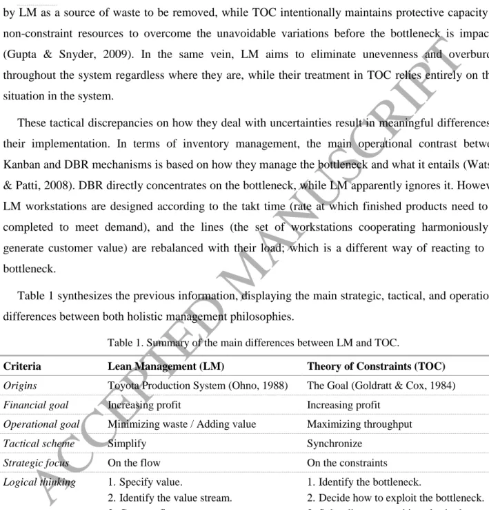
Table 1 synthesizes the previous information, displaying the main strategic, tactical, and operational differences between both holistic management philosophies.
Table 1. Summary of the main differences between LM and TOC.
Criteria Lean Management (LM) Theory of Constraints (TOC)
Origins Toyota Production System (Ohno, 1988) The Goal (Goldratt & Cox, 1984)
Financial goal Increasing profit Increasing profit
Operational goal Minimizing waste / Adding value Maximizing throughput
Tactical scheme Simplify Synchronize
Strategic focus On the flow On the constraints
Logical thinking 1.Specify value.
2.Identify the value stream. 3.Connect flow.
4.Define pull. 5.Seek perfection.
1.Identify the bottleneck.
2.Decide how to exploit the bottleneck. 3.Subordinate everything else in the
system.
4.Elevate the bottleneck. 5.Re-start the cycle.
ACCEPTED MANUSCRIPT
9
Inventory control Kanban / CONWIP4 DBR methodology
2.3. Which is the best choice? A review on comparative studies
Following from the previous discussion, both philosophies have proven to be capable of developing effective strategies for managing real-world manufacturing systems. We refer the interested reader to Achanga, Shehab, Roy, and Nelder (2006) and Mabin and Balderstone (2003), respectively, for discussions of successful implementations of LM and TOC. In light of this, several comparative studies have been conducted to explore which one performs best in various settings. This would help managers to direct redesign efforts and investment decisions.
These works generally compare LM and TOC through the performance of their scheduling mechanisms, often Kanban and DBR. In this sense, most of the relevant literature investigates serial manufacturing systems under different conditions of noise via simulation (e.g. Lambrecht & Segaert, 1990; Chakravorty & Atwater, 1996; Grunwald, Striekwold, & Weeda, 1999; Jodlbauer & Huber, 2008; Watson & Patti, 2008), while some analytical studies also deserve a mention (e.g. Takahashi, Morikawa, & Chen, 2007, who employ Markov processes). The literature review on papers comparing LM and TOC by Gupta and Snyder (2009) can be consulted for more detail.
A considerable stream of literature supports that TOC scheduling systems outperforms those of LM, such as Lambrecht and Segaert (1990), Koh and Bulfin (2004), and Watson and Patti (2008). For example, the last one explores the efficiency and robustness of production systems faced with unplanned machine downtime, and DBR achieves higher performance than Kanban in terms of total output, lead time, and inventory requirements. These authors argue that the improvement stems from the TOC system strategically protecting the bottleneck and thus achieving a higher throughput with lower inventory.
Only very few works conclude that Kanban achieves a higher performance from a broad viewpoint; e.g. Lea and Min (2003), in which TOC achieves lower customer service level with more inventory. Nonetheless, a fair amount of studies claims that each has its own region of superiority, usually depending on the noise affecting the system. For instance, Takahashi, Morikawa and Chen (2007) develop models of a Kanban system and two DBR systems that differ in the place to which orders are issued. They discuss the advantages of each system by considering the influence of processing rates
4 Constant Work-In-Progress, a pull-oriented alternative to Kanban in LM systems; see Takahashi & Nakamura (2002) for a
ACCEPTED MANUSCRIPT
10
and cost parameters. Overall, Kanban only becomes superior when the stocked items in the buffers before the bottleneck are much less costly.
Interestingly, Grunwald, Striekwold and Weeda (1989) argue that Kanban works better when the uncertainty and the complexity of the systems is relatively small, while DBR makes a difference under the opposite conditions. In a similar vein, Jodlbauer and Huber (2008) compare the service-level performance of different scheduling mechanisms. Considering a wide range of noise sources (demand, scrap, processing times, and downtimes), their results reveal that Lean’s CONWIP offers the best performance in static scenarios; however, it struggles to sustain its advantage in dynamic scenarios. In their comparative study, Chakravorty and Atwater (1996) come to the conclusion that LM production lines perform better when variability is low. However, these are heavily, negatively, impacted by variations; while the performance of DBR lines is shown to be very robust against changes. Therefore, and in line with previous works, these studies agree that TOC is more suitable to deal with uncertainty. Finally, it should be noted that several authors propose hybrid solutions, which leverage the synergies between LM and TOC, as the best solution. In this sense, Dettmer (2001) demonstrates how TOC can take the performance of those firms employing LM to the next level. Sproull (2012) discusses in detail how to integrate LM and TOC with the aim of increasing firm performance by reflecting on the strengths and weaknesses of both philosophies. Recently, Rajini, Nagaraju, and Narayanan (2018) also suggests how to effectively integrate LM and TOC for the improvement of productivity in the mining industry.
All in all, the literature provides interesting insights but contains different positions. In this regard, Gupta and Snyder (2009) underline that the results of comparative studies are still inconclusive. In the search of which system is ‘best’, they reply that no system is the ‘worst’, highlighting that each one may perform very differently in different settings.
2.4. Lean and Goldratt’s principles in the wider supply chain
As previously discussed, several prior works have compared the performance of LM and TOC placing focus on the company’s production system. This is aligned with the main use of both management philosophies in practice. However, and at the same time, several authors have underscored the value of LM and TOC principles for managing supply chains in a coordinated manner; see e.g. Naylor, Naim, and Berry (1999) or Jasti and Kodali (2015) for LM, and Perez (1997) or Simatupang and Sridharan (2004) for TOC. We strongly concur with this view. Nonetheless, some relevant
ACCEPTED MANUSCRIPT
11
differences emerge between the single-firm setting and the supply chain setting that need to be carefully addressed by managers (Puche, Ponte, Costas, Pino, & de la Fuente, 2016).
The implementation of LM and TOC in supply chains requires a certain degree of collaboration between the partners. Some important decisions need to be taken considering the interest of the whole system on the basis of greater visibility (Simatupang & Sridharan, 2002). That is, the nodes’ behavior must be oriented towards protecting the overall supply chain function, which may raise potential conflicts of interest (Mentzer et al., 2001). To prevent this from becoming a great barrier that limits the potential of the LM- or TOC-based collaborative solution, it is essential to appropriately allocate decision-making processes as well as to robustly align incentives between the partners (Simatupang & Sridharan, 2005).
Having emphasized that, the degree of collaboration required for implementing Kanban and DBR control systems for the supply chain is significantly different. While each partner can autonomously apply Kanban, a wide analysis of the supply chain is required to implement DBR for aligning processes. In this case, the relevant buffers need to be strategically placed to protect the bottleneck/s, which has strong cost implications to be considered through robust collaborative contracts. Information sharing, along with an advanced maturity level across organizational units, also becomes more important in the latter case, not only to accurately coordinate the DBR mechanism but also to define the necessary contractual agreements for aligning incentives. In light of this, the more complexity and requirements that DBR entails can be expected to result in a higher cost of implementation.
In this sense, our study contributes to the literature comparing LM and TOC by extending the comparison to the supply chain setting. To this end, we model a four-echelon supply chain faced by wide scenario of uncertainties, considering internal and external sources, through which we aim to understand the differences in supply chain performance between Kanban and DBR control mechanisms. We explore whether, and when, DBR is able to reward its added complexity, hence identifying different regions of superiority. From this viewpoint, we investigate how the findings in the supply chain buttress, or rebut, the different streams of literature previously discussed.
3. Supply chain model
Conducting an experimental study requires the prior delimitation of the scope of the problem (that is, what we consider and what we leave out). In this section, we first describe the supply chain scenario.
ACCEPTED MANUSCRIPT
12
Next, we provide a detailed explanation on how the supply chain operates with the Kanban and DBR scheduling systems. Finally, and following TOC principles, we present the economic model we employ, which defines the net profit as the key performance metric.
3.1. Supply chain scenario
The Beer Game is a role-playing exercise developed by the MIT (Jarmain, 1963) that is very effective in helping participants to explore the impact of decision making on supply chain behavior (Goodwin & Franklin, 1994). Accordingly, the scenario that this game draws up is commonly used to investigate the dynamics of such systems (Macdonald, Frommer, & Karaesmen, 2013).
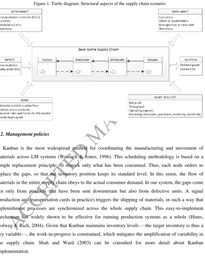
In this research, we also employ this supply chain configuration. This consists of a single-product serial production and distribution system with four echelons: factory, distributor, wholesaler, and retailer. Figure 1 displays the structural aspects of the system under consideration through a Turtle diagram. The supply chain transforms raw materials (input) into finished goods (output) to satisfy customer orders (input), which eventually become finished sales orders (output). It has two main flows: the material flow (from the supplier to the consumer, in solid lines), which relates to the product, and the information flow (in the opposite direction, in dashed lines), which includes the orders issued. To this end, the supply chain makes use of a set of resources (with what?) and is supported by a series of methodologies (how?). The figure also describes the different stakeholders involved (who?) as well as how the performance can be measured (what results?).
ACCEPTED MANUSCRIPT
13
Figure 1. Turtle diagram. Structural aspects of the supply chain scenario.
3.2. Management policies
Kanban is the most widespread method for coordinating the manufacturing and movement of materials across LM systems (Womack & Jones, 1996). This scheduling methodology is based on a simple replacement principle: to restock only what has been consumed. Thus, each node orders to replace the gaps, so that the inventory position keeps its standard level. In this sense, the flow of materials in the entire supply chain obeys to the actual consumer demand. In our system, the gaps come not only from products that have been sent downstream but also from defective units. A signal (production and transportation cards in practice) triggers the shipping of materials, in such a way that replenishment processes are synchronized across the whole supply chain. This easy-to-implement mechanism has widely shown to be effective for running production systems as a whole (Hines, Holweg & Rich, 2004). Given that Kanban maintains inventory levels —the target inventory is thus a key variable—, the work-in-progress is constrained, which mitigates the amplification of variability in the supply chain. Shah and Ward (2003) can be consulted for more detail about Kanban implementation.
ACCEPTED MANUSCRIPT
14
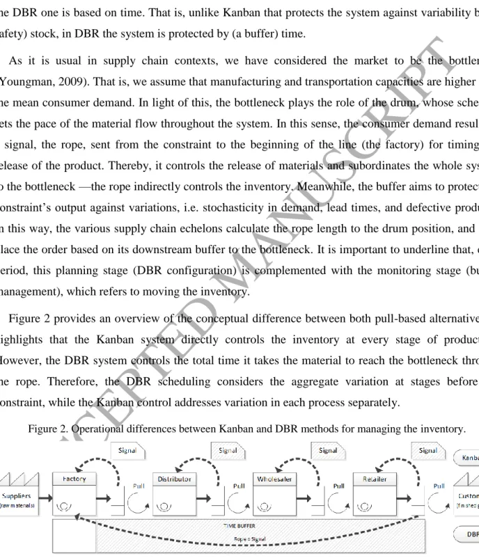
Although more complex, the DBR control idea is similar to Kanban (Watson, Blackstone, & Gardiner, 2007). However, while LM manages the bottleneck indirectly, the DBR mechanism, proposed by TOC, is directly focused on (exploiting the full capacity at) this constraint. A subtle distinction between both lies in how material is released: while Kanban method is based on inventory, the DBR one is based on time. That is, unlike Kanban that protects the system against variability by (a safety) stock, in DBR the system is protected by (a buffer) time.
As it is usual in supply chain contexts, we have considered the market to be the bottleneck (Youngman, 2009). That is, we assume that manufacturing and transportation capacities are higher than the mean consumer demand. In light of this, the bottleneck plays the role of the drum, whose schedule sets the pace of the material flow throughout the system. In this sense, the consumer demand results in a signal, the rope, sent from the constraint to the beginning of the line (the factory) for timing the release of the product. Thereby, it controls the release of materials and subordinates the whole system to the bottleneck —the rope indirectly controls the inventory. Meanwhile, the buffer aims to protect the constraint’s output against variations, i.e. stochasticity in demand, lead times, and defective products. In this way, the various supply chain echelons calculate the rope length to the drum position, and then place the order based on its downstream buffer to the bottleneck. It is important to underline that, each period, this planning stage (DBR configuration) is complemented with the monitoring stage (buffer management), which refers to moving the inventory.
Figure 2 provides an overview of the conceptual difference between both pull-based alternatives. It highlights that the Kanban system directly controls the inventory at every stage of production. However, the DBR system controls the total time it takes the material to reach the bottleneck through the rope. Therefore, the DBR scheduling considers the aggregate variation at stages before the constraint, while the Kanban control addresses variation in each process separately.
Figure 2. Operational differences between Kanban and DBR methods for managing the inventory.
ACCEPTED MANUSCRIPT
15
We compare the performance of Kanban and DBR scheduling systems from a systemic perspective. This means that we focus on the relationship between the supply chain noise and the global (instead of local) performance metrics.
The economic model that we have defined seeks to imitate the main revenues and costs faced by real-world supply chains. On the one hand, money is only made by selling finished goods to the consumer. On the other hand, expenditure is incurred by purchasing raw materials (provisioning), manufacturing products (production), transporting products (shipping), and stocking up products (storage). We assume that all of them are proportional to the volume, as this is common in the supply chain dynamics literature; see e.g. Ponte, Costas, Puche, Pino, and de la Fuente (2018). Consistently with our systemic view, we do not consider here intermediate money exchanges between the nodes (e.g. cost of intermediate goods or backlog penalties). Nonetheless, at the end of our comparative study, we will consider the issue of profit allocation, which is essential to ensure the long-term robustness of the collaborative solution.
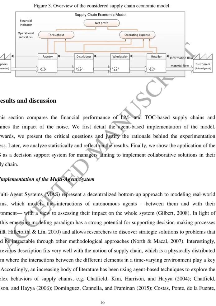
In this study, we measure the net profit as the main indicator for supply chain managers, since it quantifies the financial performance of the system in absolute terms. From this perspective, we use the Throughput Accounting (TA) (MacArthur, 1996) to obtain the net profit as the difference between the throughput and the operating expense. The throughput measures the money captured by the supply chain. It is thus calculated as the difference between the sales revenue and the provisioning costs. The operational expense refers to the money spent to turn raw material into finished products. It is obtained as the sum of production, shipping and storage costs.
Through these operational metrics, which help us to understand the variations in the net profit, the TA provides a powerful scheme to analyze the financial performance of the system. Figure 3 illustrates the relationship between the different metrics and the various supply chain nodes. Should further information be required, Youngman (2009) provides an excellent guide for using the TA.
ACCEPTED MANUSCRIPT
16
Figure 3. Overview of the considered supply chain economic model.
Factory Distributor Wholesaler Retailer
Supply Chain Economic Model
Material flow Information flow Operating expense Net profit Throughput Suppliers (raw materials) Customers (finished goods) -- + + + + Financial indicator Operational indicators + +
4. Results and discussion
This section compares the financial performance of LM- and TOC-based supply chains and examines the impact of the noise. We first detail the agent-based implementation of the model. Afterwards, we present the critical questions and justify the rationale behind the experimentation process. Later, we analyze statistically and reflect on the results. Finally, we show the application of the MAS as a decision support system for managers aiming to implement collaborative solutions in their supply chain.
4.1. Implementation of the Multi-Agent System
Multi-Agent Systems (MAS) represent a decentralized bottom-up approach to modeling real-world systems, which models the interactions of autonomous agents —between them and with their environment— with a view to assessing their impact on the whole system (Gilbert, 2008). In light of this, this emerging modeling paradigm has a strong potential for supporting decision-making processes (Lättilä, Hilletofth, & Lin, 2010) and allows researchers to discover strategic solutions to problems that would be intractable through other methodological approaches (North & Macal, 2007). Interestingly, the previous description fits very well with the notion of supply chain, which is a physically distributed system where the interactions between the different elements in a time-varying environment play a key role. Accordingly, an increasing body of literature has been using agent-based techniques to explore the complex behaviors of supply chains, e.g. Chatfield, Kim, Harrison, and Hayya (2004); Chatfield, Harrison, and Hayya (2006); Dominguez, Cannella, and Framinan (2015); Costas, Ponte, de la Fuente,
ACCEPTED MANUSCRIPT
17
Pino, and Puche (2015); Avci and Selim (2016, 2017); Ponte, Costas, Puche, de la Fuente and Pino (2016); Cannella, Dominguez, and Framinan (2017); Ponte, Sierra, de la Fuente and Lozano (2017); and Ponte, Costas, Puche, Pino and de la Fuente (2018). In this work, we also use the agent-based approach, implementing the MAS in NetLogo 5.1.0 (Wilensky, 1999).
4.1.1. The problem world and its environment
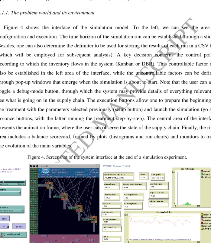
Figure 4 shows the interface of the simulation model. To the left, we can see the area of configuration and execution. The time horizon of the simulation run can be established through a slider. Besides, one can also determine the delimiter to be used for storing the results of each run in a CSV file (which will be employed for subsequent analysis). A key decision concerns the control policy according to which the inventory flows in the system (Kanban or DBR). This controllable factor can also be established in the left area of the interface, while the uncontrollable factors can be defined through pop-up windows that emerge when the simulation is about to start. Note that the user can also toggle a debug-mode button, through which the system may provide details of everything relevant to see what is going on in the supply chain. The execution buttons allow one to prepare the beginning of the treatment with the parameters selected previously (setup button) and launch the simulation (go and go-once buttons, with the latter running the treatment step-by-step). The central area of the interface presents the animation frame, where the user can observe the state of the supply chain. Finally, the right area includes a balance scorecard, formed by plots (histograms and run charts) and monitors to track the evolution of the main variables.
Figure 4. Screenshot of the system interface at the end of a simulation experiment.
ACCEPTED MANUSCRIPT
18
The animation frame depicts the Beer Game supply chain. The node agents represent the echelons of the supply chain (retailer, wholesaler, distributor and factory) and they are able to perform different activities. Each node is modeled in the form of a square, in which the agent is placed. The event agents define what happens at each moment in the supply chain. These agents, which are linked to arrival and service laws, thus trigger the action. The entity agents represent what flows in the supply chain (materials and orders). Horizontally, one finds the product channel, through which the material flows from west (factory) to east (customer). The patch closest to each node is the warehouse that keeps its on-hand inventory, while the remaining patches refer to the stock flowing towards the node. Vertically, we can see the information channel, through which the orders move from south (consumer) to north (factory). Each order travels from the sender to the receiver, who observes it once it reaches its upper patch. The record agents make annotations to calculate the KPIs of the system.
The top of the animation frame represents the space for events. To the left, one can see the sink of the system, which is used to place entities that have completed their trajectory (and will not move in the future) for traceability and statistical purposes. Finally, the bottom includes the main results of the supply chain through the relevant metrics.
4.1.3. System behavior
The MAS includes two main artifacts. First, an artifact that manages the evolution of the clock, according to the event agents that live in the Future Event List (FEL). In the FEL, new events are scheduled according to the operation of the supply chain echelons and the clock always advances to the event which is sooner due. Events work using anonymous tasks (lambdas), both to run a procedure when they are due and also to re-schedule their next arrival (due time). An event arrival asks its listeners (other agents in the system that are waiting until the event is due) to perform the scheduled activity. When these listeners are node agents they run their andon task (another lambda). To synchronize both events, the nodes takes care to have lag times so as to keep idle waiting the next demand arrival once they have completed their cycle of activity. Events are linked to their listeners by arcs in order to see what is going on in the system. There are events which are perennial; while others will die (their links also) once they are due and have completed their lambda task. It should be noted that, as usual in the Beer Game scenario, time is divided into cubes; each cube representing one day.
Second, each node is equipped with a finite-state machine artifact, which is the engine of the action. Each action leads to a state change in the finite-state machine and can generate records as well as move entities upstream or downstream (or to the sink). Therefore, actors behave like Turing machines. The
ACCEPTED MANUSCRIPT
19
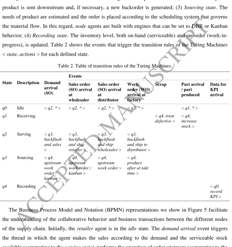
operation of the various supply chain nodes per time cube is designed according to the following five-step sequence of states: (0) Idle state. Base state, the node is waiting for new events; (1) Receiving state. The product is received from the upstream node, which increases the serviceable inventory; (2) Serving state. The order is observed and satisfied together with past backorders, if exist. Thereby, the product is sent downstream and, if necessary, a new backorder is generated; (3) Sourcing state. The needs of product are estimated and the order is placed according to the scheduling system that governs the material flow. In this regard, node agents are built with engines that can be set to DBR or Kanban behavior; (4) Recording state. The inventory level, both on-hand (serviceable) and on-order (work-in-progress), is updated. Table 2 shows the events that trigger the transition rules of the Turing Machines < state, actions > for each defined state.
Table 2. Table of transition rules of the Turing Machines.
State Description Demand
arrival (SO) Events Sales order (SO) arrival at wholesaler Sales order (SO) arrival at distributor Work order (WO) arrival at factory
Scrap Part arrival
/ part produced Data for KPI arrival q0 Idle < q2, * > < q2, * > < q2, * > < q2, * > < q1, * > q1 Receiving < q4, treat defective > < q4, increase stock > q2 Serving < q3, backflush and sales > < q3, backflush and ship retailer > < q3, backflush and ship wholesaler > < q3, backflush and ship to distributor > q3 Sourcing < q4, upstream work order | kanban > < q4, upstream work order | kanban > < q4, upstream work order > < q4, produce after at takt time > q4 Recording < q0, record KPI >
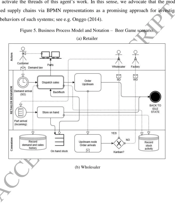
The Business Process Model and Notation (BPMN) representations we show in Figure 5 facilitate the understanding of the collaborative behavior and business transactions between the different nodes of the supply chain. Initially, the retailer agent is in the idle state. The demand arrival event triggers the thread in which the agent makes the sales according to the demand and the serviceable stock available (commuting to the serving state), performs the operation of order upstream (commuting to the sourcing state), and registers the events that occurred (commuting to the recording state). Since both LM and TOC are pull systems, the upstream demand is calculated based on the buffer management.
ACCEPTED MANUSCRIPT
20
Thus, the retailer sends it through a rope to the factory if the supply chain is operating under the DBR policy or to wholesaler if it is operating according the Kanban policy. On the other hand, in the lower thread, the orders sent upstream end up generating, after a lead time, a flow of pieces that arrive at the retailer. When the retailer is in the idle state, the node can attend this thread by commuting to receiving state. Finally, it returns to the base state (idle state) waiting for new events, which are the ones that activate the threads of this agent’s work. In this sense, we advocate that the modelling of agent-based supply chains via BPMN representations as a promising approach for investigating the complex behaviors of such systems; see e.g. Onggo (2014).
Figure 5. Business Process Model and Notation – Beer Game scenario. (a) Retailer
ACCEPTED MANUSCRIPT
21 (c) Distributor
ACCEPTED MANUSCRIPT
22
The wholesaler’s behavior is the same as that of the retailer, with the only difference that the demand is not exogenous, but it comes from the retailer. The same thing occurs with the distributor, for which the demand comes from the wholesaler. Moreover, the behavior is the same regardless of what policy is used because here the order always goes to the factory. Finally, the factory agent also presents two threads. The upper thread is dedicated to producing and leaving the product in its on-hand inventory. This thread is trigged by a clock step. In each time bucket, it decides how much to produce by following a fixed-period, variable-quantity model. If the control policy is Kanban, it will produce the gaps that have been generated in the on-hand stock since the previous time bucket; if the policy is DBR, it will produce the wear that the rope has experienced since the previous time bucket. The lower thread represents the shipping process, which sends the product downstream to replace the distributor’s consumption if the control policy is Kanban or to tight the rope from start to finish if the policy is DBR. Finally, we note if a defective piece is detected in any process, it is treated and registered by the relevant node.
In the factory, unlike the other nodes (distributor, wholesaler and retailer) in which pieces arrive as a consequence of the upstream orders or rope, the arrival of pieces does not represent an event. The pieces arrive at the end of line in the factory as an effect of having started a work order. That is, in the factory, what happens is that a work order is started because it is carried out with a fixed period, and it reacts to what happens downstream (consumption). In the rest of nodes, the events that stimulate the
ACCEPTED MANUSCRIPT
23
beginning of the process threads are the arrival of customers (sales) and the arrival of pieces as a consequence of the flow from upstream.
4.1.4. Model verification and validation
Verification and validation are essential steps in any modeling process (Kleijnen, 1995). The former involves checking that the simulation system performs as intended, i.e. it must match the rationale of the conceptual design in terms of cohesion, consistency, and stability. The latter requires checking that the results match reasonably well the real world, so that the conclusions from the analysis can be extrapolated.
For these processes, we have first used a policy of preventive quality in the modeling that consists of Test Driven Development (Beck, 2002). This is aimed at facilitating the diagnosis and is impregnated with a control plan embedded in the system as a part of the risk management to ensure the absence of bugs. This preventive quality becomes visible with cross-checks over the system’s invariants, for example: the instantiated amount of entities must match those that are still alive and those that have already died at all times; events must always be in the future and cannot form an empty set; the flow that has crossed a node fulfills the rule that what has left the node is because before it had entered in it and is no longer in the waiting queue; etc. All this set of rules is monitored by exception handler artifacts that act according to a pre-established control plan. In this way, we have tracked the behavior of the system over time in different stochastic scenarios (using both scheduling systems) to check reproducibility with confidence intervals.
Finally, we have applied Factory Acceptance Tests (Hambling & van Goethem, 2013) to confirm that the MAS exhibits the expected behavior when exposed to controlled conditions whose results are known.
4.2. Critical questions and rationale of the experimentation process
The Beer Game only considers one source of uncertainty in the previously described scenario, namely, consumer demand. From this source, together with the distortion caused by fixed lead times, the complexity of managing the system emerges. To bring this model closer to reality, we have expanded the noise scenario by considering common hurdles faced by real-world supply chains. In this regard, we adopt the following operational assumptions5: (1) Stochastic consumer demand. We use a
ACCEPTED MANUSCRIPT
24
Gauss distribution to model the demand behavior; (2) Stochastic production and transport lead times. Each node receives the product randomly (uniform distribution) within a predefined time range after it is sent by its upstream node or the production order is issued, in the case of the factory; (3) Stochastic order lead times. Each node receives the order randomly (uniform distribution) within a predefined time range after it is placed by its downstream node, except the retailer who instantly receives customers’ orders; (4) Stochastic defective products rate. When the product is being stored or transported, it may become unusable. We use a binomial distribution to represent this rate; and (5) Constrained production and transportation capacities. They follow non-parametric laws.
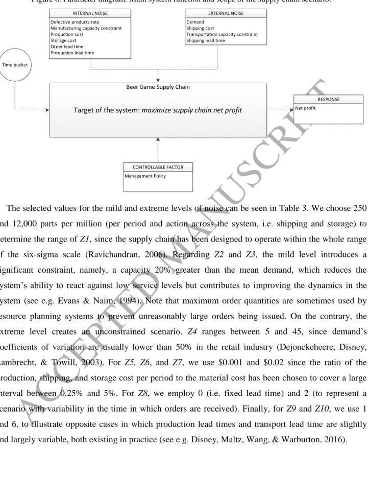
Figure 6 describes our experimentation approach in the form of a Parameter diagram that delimits the scope of our research study. This shows the noise sources (uncontrollable factors), the parameter space (controllable factors), and the measurement of the system response. The noise has been divided into external noise and internal noise, which establishes a difference between those sources generated inside and outside the supply chain. The parameter space includes the management approach (Kanban or DBR), which is the main factor whose response we aim to investigate. Meanwhile, the main system function is to transform the customer demand (mean of the demand) and selling price (gross margin per unit of product) into financial performance, thus measuring its response through the net profit.
Mathematically, this experimentation approach can be expressed by Y=f(X,Z)+ξ. This expresses the system response (Y), or net profit, as a function of the controllable factor (X), representing the scheduling mechanism, and a compound noise (Z), which encompasses all the uncontrollable factors that threaten the efficiency of the supply chain, plus the residuals (ξ), which consider the unexplained part of the system response. Additionally, the supply chain noise is established as a compound of ten factors; thence, it may be expressed as Z={Z1,Z2,Z3,Z4,Z5,Z6,Z7,Z8,Z9,Z10}. These are: defective products rate (Z1), transportation capacity constraint (Z2), manufacturing capacity constraint (Z3), demand (Z4), production cost (Z5), shipping cost (Z6), storage cost (Z7), order lead time (Z8), production lead time (Z9), and shipping lead time (Z10).
ACCEPTED MANUSCRIPT
25
Figure 6. Parameter diagram. Main system function and scope of the supply chain scenario.
Beer Game Supply Chain
Management Policy CONTROLLABLE FACTOR Defective products rate
Manufacturing capacity constraint Production cost
Storage cost Order lead time Production lead time
INTERNAL NOISE
Demand Shipping cost
Transportation capacity constraint Shipping lead time
EXTERNAL NOISE
Net profit RESPONSE
Target of the system: maximize supply chain net profit
Time bucket
The selected values for the mild and extreme levels of noise can be seen in Table 3. We choose 250 and 12,000 parts per million (per period and action across the system, i.e. shipping and storage) to determine the range of Z1, since the supply chain has been designed to operate within the whole range of the six-sigma scale (Ravichandran, 2006). Regarding Z2 and Z3, the mild level introduces a significant constraint, namely, a capacity 20% greater than the mean demand, which reduces the system’s ability to react against low service levels but contributes to improving the dynamics in the system (see e.g. Evans & Naim, 1994). Note that maximum order quantities are sometimes used by resource planning systems to prevent unreasonably large orders being issued. On the contrary, the extreme level creates an unconstrained scenario. Z4 ranges between 5 and 45, since demand’s coefficients of variation are usually lower than 50% in the retail industry (Dejonckeheere, Disney, Lambrecht, & Towill, 2003). For Z5, Z6, and Z7, we use $0.001 and $0.02 since the ratio of the production, shipping, and storage cost per period to the material cost has been chosen to cover a large interval between 0.25% and 5%. For Z8, we employ 0 (i.e. fixed lead time) and 2 (to represent a scenario with variability in the time in which orders are received). Finally, for Z9 and Z10, we use 1 and 6, to illustrate opposite cases in which production lead times and transport lead time are slightly and largely variable, both existing in practice (see e.g. Disney, Maltz, Wang, & Warburton, 2016).
ACCEPTED MANUSCRIPT
26
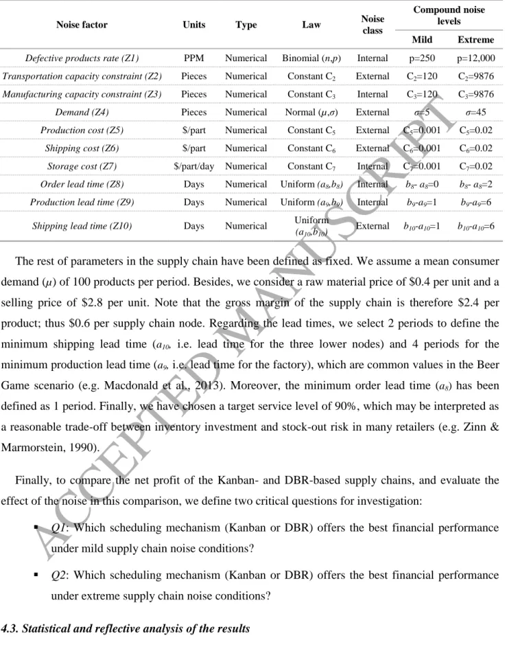
Table 3. Definition of the noise factors and compound noise levels.
Noise factor Units Type Law Noise
class
Compound noise levels
Mild Extreme
Defective products rate (Z1) PPM Numerical Binomial (n,p) Internal p=250 p=12,000
Transportation capacity constraint (Z2) Pieces Numerical Constant C2 External C2=120 C2=9876
Manufacturing capacity constraint (Z3) Pieces Numerical Constant C3 Internal C3=120 C3=9876
Demand (Z4) Pieces Numerical Normal (µ,σ) External σ=5 σ=45
Production cost (Z5) $/part Numerical Constant C5 External C5=0.001 C5=0.02
Shipping cost (Z6) $/part Numerical Constant C6 External C6=0.001 C6=0.02
Storage cost (Z7) $/part/day Numerical Constant C7 Internal C7=0.001 C7=0.02
Order lead time (Z8) Days Numerical Uniform (a8,b8) Internal b8- a8=0 b8- a8=2
Production lead time (Z9) Days Numerical Uniform (a9,b9) Internal b9-a9=1 b9-a9=6
Shipping lead time (Z10) Days Numerical Uniform
(a10,b10)
External b10-a10=1 b10-a10=6
The rest of parameters in the supply chain have been defined as fixed. We assume a mean consumer demand (µ) of 100 products per period. Besides, we consider a raw material price of $0.4 per unit and a selling price of $2.8 per unit. Note that the gross margin of the supply chain is therefore $2.4 per product; thus $0.6 per supply chain node. Regarding the lead times, we select 2 periods to define the minimum shipping lead time (a10, i.e. lead time for the three lower nodes) and 4 periods for the minimum production lead time (a9, i.e. lead time for the factory), which are common values in the Beer Game scenario (e.g. Macdonald et al., 2013). Moreover, the minimum order lead time (a8) has been defined as 1 period. Finally, we have chosen a target service level of 90%, which may be interpreted as a reasonable trade-off between inventory investment and stock-out risk in many retailers (e.g. Zinn & Marmorstein, 1990).
Finally, to compare the net profit of the Kanban- and DBR-based supply chains, and evaluate the effect of the noise in this comparison, we define two critical questions for investigation:
Q1: Which scheduling mechanism (Kanban or DBR) offers the best financial performance under mild supply chain noise conditions?
Q2: Which scheduling mechanism (Kanban or DBR) offers the best financial performance under extreme supply chain noise conditions?
ACCEPTED MANUSCRIPT
27
Since we have defined two levels for both the controllable factor X (Kanban or DBR) and the compound noise Z (mild or extreme), four treatments can be obtained (i.e. DBR-mild, DBR-extreme, Kanban-mild, and Kanban-extreme). Each treatment has been replicated five times. Thus, we obtain a total of 20 runs. A time horizon of 200 periods has been selected for each run, which has proven to be enough to have the MAS working under steady-state conditions after a warm-up period of 30 days.
Table 4. Results of the simulation runs.
Replica Run Management policy Compound noise Net profit [$]
1 01 DBR Mild $45,575.07 02 DBR Extreme $33,324.14 03 Kanban Mild $46,262.84 04 Kanban Extreme $30,749.99 2 05 DBR Mild $45,551.44 06 DBR Extreme $30,709.68 07 Kanban Mild $46,325.51 08 Kanban Extreme $31,760.57 3 09 DBR Mild $45,673.93 10 DBR Extreme $34,120.47 11 Kanban Mild $46,319.06 12 Kanban Extreme $28,248.33 4 13 DBR Mild $45,929.13 14 DBR Extreme $33,457.73 15 Kanban Mild $46,252.22 16 Kanban Extreme $31,540.38 5 17 DBR Mild $45,791.85 18 DBR Extreme $33,697.97 19 Kanban Mild $46,421.90 20 Kanban Extreme $29,575.24
Table 4 shows the numerical results, through the net profit of the four-echelon supply chain, of the 20 simulations runs that we have performed. The statistical analysis detailed below has been carried out with JMP© v.10 software (Sall, Lehman, Stephens, & Creighton, 2012).
To evaluate the impact of the management policy (X) and the compound noise (Z), and their interactions, on the net profit of the supply chain (Y), we conduct a two-way analysis of variance (ANOVA) with interactions. We first need to highlight that, from a statistical viewpoint, the model
ACCEPTED MANUSCRIPT
28
exhibits a good fit with the data; see Figure 7. As the adjusted coefficient of determination is considerably high (R2adj = 0.982032), the variability explained by the model is much higher than that absorbed by the residual. The analysis of variance confirms that the model is relevant (p-value<<5%). It can be also seen in the effect tests that the compound noise and the management policy independently are statistically significant (p-values<5%). Finally, and central to the purpose of our study, the interaction between these parameters is also significant (p-value<<5%).
Figure 7. Summary of two-way ANOVA with interactions results (Notation - NP: net profit; MP: management policy; CN: compound noise).
The interaction profiles in Figure 7 suggest that, when the supply chain noise is extreme, the implementation of the DBR mechanism results in a significantly higher net profit than the implementation of Kanban. However, under mild noise conditions, it seems that the financial performance of the supply chain is similar in both cases —we may even observe that performance of Kanban is slightly higher.
To this end, Figure 8 provides an analysis of the difference of means through the Tukey’s HSD (honestly significant difference) test. We focus on the following combinations: first, extreme-DBR and extreme-Kanban; and, second, mild-DBR and mild-Kanban. In the former, the difference is statistically significant (p-value=0.0031<5%) and the average difference is $2,867.1. In the latter, the average
ACCEPTED MANUSCRIPT
29
difference decreases to $612.02; the net profit being higher in Kanban. However, this difference is not found to be significant (p-value=0.7690>>5%). Overall, we fail to reject the null hypothesis for Q1 (power: 0.9334), and we reject the null hypothesis for Q2. Consequently, we may conclude that in mild noise conditions the DBR mechanism provides the same net profit as the Kanban control system, while in extreme conditions, DBR makes a difference and offers a higher financial performance than Kanban.
Figure 8. Summary of the LSMeans Tukey HSD test and Principal Components Analysis.
Having verified the statistical significance between the net profit of both supply chains when the noise is extreme, an important question arises from a managerial perspective. This concerns evaluating if this difference is relevant enough to justify the practical implementation of the DBR scheduling methodology in supply chains, knowing that it tends to be significantly more costly than the implementation of the Kanban mechanism. When we compare this difference ($2,687.1) to the total net profit ($31,718.45, calculated as the average of extreme-DBR and extreme-Kanban), a potential increase in net profit of 8.47% may be interpreted as high enough to advise the implementation of DBR instead of Kanban in these contexts of severe noise. However, and in line with the previous discussion, Kanban proves to be a more appropriate alternative when the supply chain noise is low, given that it offers a similar performance at a significantly lower implementation cost and effort.
To better interpret the results, we look at both components of the net profit. As previously discussed, the TA expresses this metric as the difference between the throughput and the operating expense. Looking at the means of the different groups in Figure 8, this suggests that the DBR system is able to
ACCEPTED MANUSCRIPT
30
increase the throughput of the supply chain. In this regard, the Principal Components Analysis of Figure 8 shows that the first component, i.e. the throughput, explains 71.297% of the total variance in the net profit, while the second component, i.e. the operating expense, provides an explanation for the remaining 28.703%. We highlight that these findings link perfectly with the TOC philosophy. The throughput increase is reasonable due to the fact that the DBR scheduling mechanism manages the inventory with a clear bottleneck orientation. Indeed, increasing the throughput is a core objective under the TOC approach.
4.4. On the decision-making value of the Multi-Agent System: A motivating application
To illustrate the contribution of this work in terms of supply chain decision making, let us assume that the supply chain under consideration is currently operating according to a Kanban policy in a scenario characterized by long lead times and high uncertainty. In this initial state, the only necessary negotiation among the supply chain partners is the price policy agreed to launch the supply chain. We consider that the following distribution of the overall gross margin has been agreed: factory – 25% ($0.60), distributor - 15% ($0.36), wholesaler – 22.5% ($0.54), and retailer – 37.5% ($0.90). Considering that the raw material price has been defined as $0.40 and the selling price (to consumers) is $2.8 —see Section 4.2 for more detail—, this would result in the following intermediate prices: $1.00 (from factory to distributor), $1.36 (from distributor to wholesaler), and $1.90 (from wholesaler to retailer).
Let us also assume that supply chain stakeholders have employed the Multi-Agent System to discover the overall benefits derived from moving towards a DBR mechanism under such noise conditions. Nevertheless, the fact that the supply chain makes more money when using the DBR methodology does not necessarily imply that every node will naturally increase their net profit. Indeed, the DBR mechanism may create some inequalities in the supply chain due to its bottleneck orientation. Specifically, the retailer —who directly deals with the bottleneck— may need to invest in higher inventories to protect the supply chain service level, which would have a negative impact on its financial performance. Therefore, supply chain actors would soon realize that the design of an appropriate, self-enforcing, incentive alignment scheme emerges as a key aspect for ensuring the viability of the DBR-based supply chain.
The first numerical column of Table 5 shows the average net profit of each supply chain member in the simulations carried out in the extreme noise scenario (i.e., runs 4, 8, 12, 16, and 20). It is interesting to note that the differences in the net profit between the echelons mainly emerge because of two