Evolutionary Optimization for Safe Navigation of an Autonomous Robot in Cluttered Dynamic Unknown Environments

(1)

Cleveland State University

EngagedScholarship@CSU

ETD Archive

2018

Evolutionary Optimization for Safe Navigation of

an Autonomous Robot in Cluttered Dynamic

Unknown Environments

Arash Roshanineshat

Cleveland State University

Follow this and additional works at:https://engagedscholarship.csuohio.edu/etdarchive

Part of theElectrical and Computer Engineering Commons How does access to this work benefit you? Let us know!

This Thesis is brought to you for free and open access by EngagedScholarship@CSU. It has been accepted for inclusion in ETD Archive by an authorized administrator of EngagedScholarship@CSU. For more information, please [email protected].

Recommended Citation

Roshanineshat, Arash, "Evolutionary Optimization for Safe Navigation of an Autonomous Robot in Cluttered Dynamic Unknown Environments" (2018).ETD Archive. 1081.

(2)

Evolutionary Optimization for Safe Navigation of an Autonomous Robot in Cluttered Dynamic Unknown

Environments

ARASH ROSHANINESHAT

Bachelor of Science in Electrical Engineering University of Zanjan

June 2015

submitted in partial fulfillment of requirements for the degree MASTER OF SCIENCE IN ELECTRICAL ENGINEERING

at the

CLEVELAND STATE UNIVERSITY August 2018

(3)

We hereby approve this thesis for ARASH ROSHANINESHAT

Candidate for the Master of Science in Electrical Engineering degree for the Department of Electrical Engineering and Computer Science

and the CLEVELAND STATE UNIVERSITY’S College of Graduate Studies by

Thesis Chairperson, Dr. Dan Simon

Department & Date

Thesis Committee Member, Dr. Lili Dong

Department & Date

Thesis Committee Member, Dr. Mohammad Shokrolah Shirazi

Department & Date

(4)

ACKNOWLEDGMENTS

I would like to express my sincere gratitude to my advisor, Prof. Dan Simon, for his continuous, invaluable guidance and patience in my work. His motivation, creative problem-solving skills and immense knowledge were gifts that I hope I can embody. I thank Taylor Barto, Saman Khademi, Seyed Fakoorian, Haniye Mohammadi, Donald Ebeigbe and Mohamed Abdelhady for their help and support throughout my project and research as lab mates, and for being there when I needed them. I also would like to thank Dr. Jonathan Weintroub for mentoring my internship at Harvard-Smithsonian, and Dr. Richard Prestage for advising my internship at National Radio Astronomy Observatory. I appreciate their encouragement and support for my projects, which helped me develop programming and problem-solving skills. I want to thank Saba, Leili, Ashkan and my friends at Cleveland State University for providing joy and laughter at the right time when I needed them. I thank the people at the IEEE section of Cleveland State University who let me be involved in several robotic and volunteering opportunities. Last but most of all, I would like to thank my parents and my sister, who always tried to sacrificially help and support me through the years and who were there for me even though I am thousands of miles away.

(5)

Evolutionary Optimization for Safe Navigation of an Autonomous Robot in Cluttered Dynamic Unknown Environments

ARASH ROSHANINESHAT

ABSTRACT

We present a path planning approach based on probabilistic methods for a robot to navigate in a cluttered, dynamic, unknown environment. There are dynamic obsta-cles moving around and static obstaobsta-cles located in the map. The robot does not have any prior information about them but should be able to navigate through the map beginning from a known starting point and safely ending at a known target point. The only information the robot has is the location of the starting point and the target point and it uses sensory information to collect information about its surroundings. Our method is compared to the D* Lite algorithm and results are presented. In the last section, the parameters of the robot are optimized using biogeography-based op-timization (BBO). This is an efficient multivariable optimizer and it is shown that the results of optimization achieve significant improvement in robot navigation per-formance. In this thesis, we show that using evolutionary optimization methods like BBO can reduce the risk of collision and the navigation time by about 25% each. The resulting risk of collision indicates safe navigation by the robot which leads to the conclusion that this is a feasible method for real-world robots.

(6)

TABLE OF CONTENTS

Page

ABSTRACT . . . iv

LIST OF TABLES . . . vii

LIST OF FIGURES . . . viii

CHAPTER I. INTRODUCTION . . . 1

II. PROBABILISTIC PATH PLANNING . . . 7

2.1. Radar System . . . 9

2.1.1. Circular Obstacles . . . 12

2.1.2. Obstacles composed of straight lines . . . 14

2.2. Target Distribution dT . . . 16

2.3. Obstacle Distribution dO . . . 17

2.4. Final target distribution dF . . . 19

2.5. Memory Distribution dM . . . 22

2.6. Final Robot Steering Direction: Combining dM and dF . . . 24

III. The D* ALGORITHM . . . 27

3.1. Algorithm . . . 27

3.2. Lifelong Planning A* (LPA*) . . . 30

3.3. D* Lite . . . 33

3.4. Experimental Results . . . 36

(7)

V. SIMULATION RESULTS . . . 44

5.1. Only Dynamic Obstacles, No Bouncing after Collisions . . . 44

5.2. Only Dynamic Obstacles, With Bouncing . . . 47

5.3. Simple Maze with Dynamic Obstacles . . . 52

5.4. Map with Rooms . . . 55

VI. CONCLUSION . . . 60

BIBLIOGRAPHY . . . 62

APPENDICES A. Box2D Library . . . 67

(8)

LIST OF TABLES

Table Page

I. Speed modes; see Figure 10 for regions. . . 21 II. Memory size comparison for various lengths of time for which the robot

will save previously visited points. The nominal value in this thesis is 8 seconds. . . 24 III. Functions of priority vertices queue U . . . 31 IV. Comparison between D* Lite and the probabilistic method . . . 38 V. Optimized parameters for the map of Figure 23. TS stands for time step. 47 VI. Optimized parameters for the map of Figure 28. TS stands for time step. 51 VII. Optimized parameters for the map of Figure 33. TS stands for time step. 53 VIII. Optimized parameters for the map of Figure 38. TS stands for time step. 58

(9)

LIST OF FIGURES

Figure Page

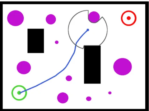
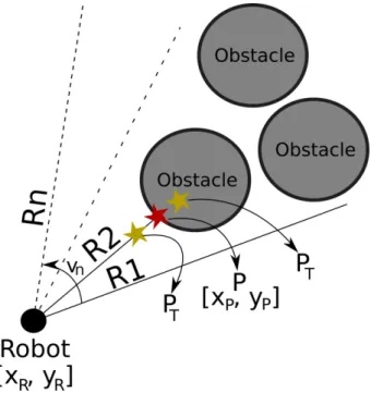
1. Sample map with static obstacles in black and dynamic obstacles in pink. Dark gray shows the radar range, the red symbol in the upper right shows the target point and the blue line shows the path of the robot starting from the initial point at the lower left, which is marked in green. . . . 8 2. Laser beam rays are denoted as R1,R2,· · ·, Rn. The approximate

inter-section points of the radar with the obstacle are denoted as PT, which,

because of the radar resolution, is not the same as the exact intersection point P. νn is the angle of laser beam n with the horizontal axis. . . 10

3. A sample ray of the laser beam and the steps that the simulator uses to check whether each point along the beam is free space or occupied by an obstacle. . . 12 4. Intersection of a line segment, which denotes the robot radar beam, and

a circular obstacle. . . 13 5. The corners of a rectangular obstacle are denoted as C1, C2, C3 and C4.

The positions of the corners are know to the simulator. The intersections of the beam ray R and the obstacle are denoted as Z1 and Z2. . . 15 6. Sample memory array returned by the radar system. This memory array

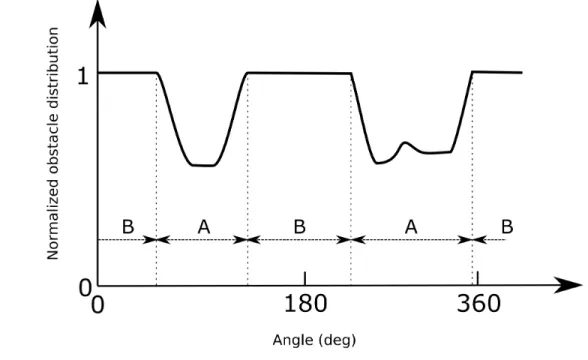
contains 360 entries, one for each degree of radar resolution. . . 16 7. Two target distributions with different σ values. . . 17 8. Obstacle distribution d0. There are two types of regions in this figure: A

indicates the existence of obstacles at the given angles, and B indicates that there are no obstacles at the given angles. . . 19

(10)

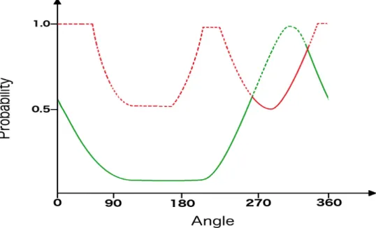
9. Example of final target distribution construction. The original target distribution is green and the obstacle distribution is red. The solid line is the final target distribution and is constructed by taking the minimum value of the original target distribution and the obstacle distribution. . . 20 10. Different speed mode regions that the robot uses to change its speed

according to the position of the closest obstacle. . . 21 11. Memory queue in which previously visited coordinates are stored. . . 22 12. Illustration of memory points (MPs). The dashed lines show the direction

of the repulsive force imparted to the robot by each MP. . . 23 13. Memory distribution based on recently visited locations. . . 23 14. Illustration of dF and dM vectors and their weighted summation vector,

which is the final robot steering direction. . . 25 15. Illustration of how the speed of the robot changes with time based on

sensed obstacles. . . 26 16. Illustration of how the robot moves toward the target while avoiding

obstacles. . . 26 17. Sample tile map and A* navigation. The robot’s initial point is indicated

with an R and the target point is indicated with a T. State O shows a tile in the graph whose state (open or closed) the robot does not know. Gray static obstacles are known to the robot prior to path planning. Arrows show the optimum path to the target point as computed by the A* algorithm based on prior knowledge of the map. . . 29 18. An updated version of Figure 17 using D* Lite. The arrows have been

been updated and the blocked gate between the two obstacles has been resolved. . . 35 19. Maps used to compare the results for the probabilistic method and the

(11)

20. Biogeography migration of species to islands with lower habitat suitability index . . . 40 21. Depiction of how the time and collision cost functions are combined. The

first m elements all have a time cost function less than a given threshold and are then sorted according to the number of collisions. The lastn−m elements all have a time cost function greater than the threshold and are sorted according to time. . . 42 22. Block diagram of BBO algorithm . . . 43 23. This map shows the robot and a sample trajectory from the starting point

to the target point. The map contains only dynamic obstacles. In this map there is no bouncing after collisions. . . 45 24. Distance from the robot to the target as a function of time for a sample

simulation of the map of Figure 23. . . 46 25. Robot speed as a function of time for a sample simulation of the map of

Figure 23. . . 46 26. The number of collisions for Figure 23 improves by optimizing the path

planning algorithm parameters with BBO. The number of collisions is averaged over eight Monte Carlo simulations. . . 48 27. The number of time steps required to reach the target in Figure 23

im-proves by optimizing the path planning algorithm parameters with BBO. The number of collisions is averaged over eight Monte Carlo simulations. 48 28. This map shows the robot and a sample trajectory from the starting point

to the target point. The map contains only dynamic obstacles. In this map there is bouncing after collisions. . . 49 29. Distance from the robot to the target as a function of time for a sample

(12)

30. Robot speed as a function of time for a sample simulation of the map of Figure 28. . . 50 31. The number of collisions for Figure 28 improves by optimizing the path

to the target point. The map contains only dynamic obstacles. Bouncing after collisions is enabled. . . 53 34. Distance from the robot to the target as a function of time for a sample

simulation of the map of Figure 33. . . 54 35. Robot speed as a function of time for a sample simulation of the map of

Figure 33. . . 54 36. The number of collisions for Figure 33 improves by optimizing the path

to the target point. The map contains several rooms in which the robot tends to get stuck. Bouncing after collisions is enabled. . . 56 39. Distance from the robot to the target as a function of time for a sample

(13)

40. Robot speed as a function of time for a sample simulation of the map of Figure 38. . . 58 41. The number of collisions for Figure 38 improves by optimizing the path

im-proves by optimizing the path planning algorithm parameters with BBO. The number of collisions is averaged over eight Monte Carlo simulations. 59 43. Overview of an object decleration in Box2D . . . 68 44. Block diagram of the operation of the SFML . . . 70

(14)

CHAPTER I INTRODUCTION

Mobile robots have been become increasingly popular in automated indus-trial environments. Surveillance, Mars explorers, and underwater exploration are other applications of mobile robots. In many situations, the robot doesn’t have prior knowledge about the environment and providing this information is either difficult or impossible. In all of these applications collision-free path planning is an impor-tant necessity. Furthermore, using a robot in any of the aforementioned situations is acceptable only if the robot provides high efficiency and low cost. High efficiency can defined as fast customer service, low power consumption and low maintenance costs. Therefore, the robot should have the ability to autonomously find a path with a minimum risk of collision and high efficiency with no knowledge, or with minimum knowledge, about the surrounding environment. This chapter reviews previous work and research that has been done to make robot navigation safe and efficient.

Path planning algorithms are also used in applications other than robot navi-gation. In [25], the authors used path planning algorithms to find hierarchical routes for networks in wireless mobile communication. The authors in [6] used sampling-based path planning algorithms to define flexible molecular models as conformational filters with energy refinement to provide a geometric interpretation of constraints affecting molecular motion. They claimed that they developed new techniques for better exploitation of the geometric path information provided in the first filtering

(15)

stage. Kinematic chains are introduced in [23] as a ubiquitous representation of bi-ological macro-molecule motion. In both robotic and bibi-ological applications of path planning, methods can benefit from a collision detection system. In [23] the authors used various benchmarks in their research and claim to have found a novel kinematic chain representation for fast detection of self-collision. Furthermore, they concluded that their approach can be used in both robotics and molecular biology. Collision detection is also important in computer animation. When several graphical objects move on a computer screen, they may interfere with each other and need to react appropriately. This is especially important if we want to have realistic collision be-havior. Detecting collisions accurately is a time consuming process so designing a dynamic simulation system is required to handle this issue [26].

The motion planning problem involves searching in the configuration space of a complex geometric rigid body that connects a starting point to a destination point through a collision free path [22]. This path should satisfy the constraints imposed by other rigid bodies or obstacles in the environment. There are complete methods to solve general problems [30,3] but they are known for their computational complexity and computing demands. So this limits the possibly of using them for even low-dimensional configuration spaces. In [22], the authors conclude that a randomized approach called rapidly-exploring random trees (RRTs) in single-query motion plan-ning yields good performance for a wide range of problems and applications. They claim that their method is probabilistically complete and is suitable for incremental distance computation algorithms. In [22] the authors improve the robot’s behavior by optimizing the RRT step sizes.

Service robots in uncertain environments have become very popular in the last few years. A variety of systems exist in places like hospitals, office buildings, department stores, and museums. As mentioned earlier, for robots to be capable team members and helpful assistants, especially in dynamic human-populated

(16)

envi-ronments, they need to navigate efficiently and safely. Recall that efficiency is defined as the ability of a robot to reach a target point from a starting position in a prior unknown environment in a short time period, and safety is defined as the number of collisions a robot may have with obstacles (e.g., humans) during navigation to the target point. Robot motion planning in dynamic environments has recently received substantial attention due to the advent of autonomous cars and the growing interest in social, service, and assistive robots.

In [9], the authors focus on learning a robot path for ease of movement, and detecting and avoiding obstacles using a single camera and a laser source. In [28] the authors propose a hybrid potential field, which can be computed in real time, to navigate in a dynamic environment with 50 randomly moving obstacles. A fuzzy inference system with an accelerate / break module is developed in [35] for real-time navigation of autonomous underwater vehicles in both static and dynamic three-dimensional environments while automatically avoiding the dynamic obstacles using sonar, along with virtual acceleration and velocity in both the horizontal and vertical plane. In [17], a fuzzy truck control system for obstacle avoidance with reasonably good trajectory is proposed, using 33 fuzzy inference rules for steering control and 13 rules for speed control. In [13], two fuzzy logic controllers for steering and velocity control of an autonomous vehicle are divided into seven control modules. This leads to the generation of a path to the target point, including desired orientation, while avoiding collisions with obstacles, driving the vehicle through mazes, and controlling the velocity based on the obstacles in the map and based on the need to navigate around sharp corners.

A novel algorithm for collision free navigation in complex dynamic environ-ments with moving obstacles is proposed in [29]. The algorithm considers an inte-grated representation of the environment by approximating the shape of the obsta-cles in the map by cirobsta-cles and polygons. This reduces the required computational

(17)

effort and increases the speed of the simulations. The navigation algorithm provides minimum-distance path planning through a crowd of moving or stationary obsta-cles [29].

An efficient stereovision-based motion compensation method for moving robots is presented in [15] using the disparity map and three modules: segmentation, feature extraction, and estimation. In the segmentation module, the authors propose the use of extended type-2 fuzzy information theory to recognize the obstacles. Fuzzy logic is used to implement the design and coordination [36] of a memory grid and to develop a minimum risk method for robot navigation, and is able to avoid collision with obsta-cles in different scenarios, such as long walls, large concave and recursive UU-shaped regions, unstructured regions, cluttered regions, and maze-like obstacles that repre-sent dynamic indoor environments. In [1] a fuzzy logic controller is developed based on the Mamdani-type fuzzy method for robot navigation and obstacle avoidance in a cluttered environment. A fuzzy controller with three inputs and a single output pro-vides safe navigation for the robot motion in a static environment while taking into account the accuracy of the measurements of its position, distance to the obstacles and the goal point, speed, orientation, and the rate of change of its heading angle. The authors in [1] describe a fast and reliable method of obstacle avoidance for both for outdoor and indoor navigation. The method is applicable in various mobile robotic systems regardless of whic sensors are used and is based on two complementary ap-proaches: non-complex implementation and human-like smooth steering. In [37] a conceptual approach is considered based on fuzzy logic to solve the local navigation and obstacle avoidance problem for multi-link robots. The fuzzy rule-based approach is considered as an on-line local navigation method for the generation of instantaneous collision-free trajectories.

The above papers use fuzzy approaches, but there has also been research with probabilistic approaches. In [16], the authors proposed a method in which a

(18)

multi-degree of freedom robot uses two-step path planning: the first step uses a probabilistic method to generate all possible paths between its configurations, and the next step, the query phase, connects the generated paths between two nodes and selects the best path. This method was experimentally demonstrated with pre-known static maps. Rapidly-exploring random trees(RRTs) are introduced in [22]. RRTs incrementally generate new nodes from the starting node to the ending node. The nodes explore the map using simple greedy heuristics.

Path planning algorithms can be optimized using different algorithms. In general, optimization means selecting the best variables relative to some criterion from a set of available options. Selecting the best variables will cause a function called the cost function to be maximized or minimized.

Many approaches have been developed to optimize motion planning algo-rithms. Common motion planning algorithms produce inefficient trajectories for high dimensional and complex dynamics [8,18,5]. There are various methods for optimiza-tion; genetic algorithms, particle swarm optimization (PSO) and biogeography-based optimization (BBO) are a few of them. In this thesis, BBO is used as the optimiza-tion method. PSO individuals tend to clump together, but BBO doesn’t have that limitation [31].

There are uncertainties in all evolutionary algorithms. The first type of un-certainty is caused by the noise of the cost function evalution, which can have many different sources, such as noise from measurement sensors. The second type of un-certainty is caused by the nondeterministic behavior of the environment. This means that environmental parameters change with time and optimization should be robust enough to adapt to new parameters. The environment can vary after the optimum values are found, but the optimum parameter values should still give satisfactory results. The third type of uncertainty comes from the approximation of the cost function. The cost function is estimated by the most feasible and appropriate form

(19)

(meta-model) due to the complexity and difficulty of using the actual cost function. This will add errors and uncertainties. For the last type of uncertainty, systems need to be continuously optimized. The optimizer should be able to track the optimum pa-rameter values over time. The challenge here is to use previously generated optimum values to speed up the new optimization process [14].

Contribution of this Research

In this research, a probabilistic method is introduced for path planning. This method is fast, real-time and can be extended to various types of autonomous robots. It can be used for autonomous underwater exploration and the same algorithm can used for autonomous drones. The robot uses a minimal amount of memory.

To optimize the path planning algorithm, the parameters of the method are tuned using biogeography-based optimization (BBO). The BBO method in this re-search optimizes 14 parameters for the path planning algorithm.

(20)

CHAPTER II

PROBABILISTIC PATH PLANNING

This chapter describes our new probabilistic path planning algorithm. The path planning problem is set in a two dimensional map, in which the robot is trying to move from a starting point to an arbitrary but known target point. The robot does not have prior knowledge about the shape, location and size of the obstacles in the map and so it begins by hypothesizing that the path to the target point is a straight line from its current location.

The map is treated as a continuous environment and the location of the ob-stacles and the robot is determined in (x, y) coordinates. The map contains dynamic and static obstacles, an example of which is shown in Figure 1. The robot is equipped with a 360◦range-limited radar sensor that is used to find the distance to the obstacles around the robot. The radar system is explained in detail in the next section. The robot also has the ability to instantaneously change its velocity to avoid collisions.

The objective of the robot is to find a minimum-time trajectory starting from the initial point on the map to the target point while minimizing the probability of collision with the static and dynamic obstacles.

We assume for now that the robot has a perfect sense of its current location as well as the location of the target point. The robot will determine the heading angle α with which to reach the target point if there were no obstacles in the way. However, there are might be unknown obstacles on the way and the robot needs

(21)

Figure 1: Sample map with static obstacles in black and dynamic obstacles in pink. Dark gray shows the radar range, the red symbol in the upper right shows the target point and the blue line shows the path of the robot starting from the initial point at the lower left, which is marked in green.

to react accordingly. So, in our algorithm, the robot creates a normal Gaussian distribution dT centered at α with a dynamic adjustable standard deviation σ. The

robot uses a function fθ to return the argument of the maximum value of an input

distribution as the best angle to travel to avoid colliding with obstacles. The output of fθ with dT as its input is clearly α.

fθ(dT) = argmax(dT) =α (2.1)

The probabilistic algorithm dictates that the robot choose an angle Θ to direct the robot to the target point in a way that has the lowest probability of colliding with an obstacle, or in other words, has the highest probability of reaching the destination without a collision. To find Θ, we construct three distributions; one isdT as mentioned

above, which we call the target distribution. The target distribution is created on the basis of the current location of the robot and the target point is Gaussian with center

(22)

α. The second distribution is called the obstacle distribution, dO, and is created

based on the obstacles detected by the robot’s radar. The third distribution is called the memory distribution, dM, and uses locations that have been previously visited by

the robot to create a Gaussian distribution. This distribution helps the robot escape rooms or blocked areas by backtracking.

2.1 Radar System

The robot does not know anything about its environment except the informa-tion that it obtains from its radar. The robot is equipped with a 360◦ radar that it uses to obtain information about its surrounding area, including both static and dy-namic obstacles. Each time step, the radar rotates once and collects 360 data points, one data point per degree. That is, the radar is configured with a 1◦ resolution.

This arrangement is shown in Figure 2. The robot coordinates are denoted as [XR, YR]. In practice, the laser beam emits a ray and as the ray bounces from

an obstacle, the sensor measures the distance based on the elapsed time. However, in simulation, the distance of the robot to an obstacle is calculated with geometric equations.

Although the robot has no prior information about the obstacles or the en-vironment, the simulator has complete information for all objects in the simulation. So the robot emits the laser beam and then the simulation program provides the distance to each obstacle. This approach makes it possible to have modular code that can be easily ported and converted to a real-world application. Because the path planning algorithm does not need to know anything about how its radar works, the robot can simply request the distance to the closest obstacle at a specific angle and then wait for the answer from either the simulator or the radar module. Therefore, the obstacle distance can be generated using either the simulator or a real-world laser beam sensor.

(23)

Figure 2: Laser beam rays are denoted as R1, R2, · · ·, Rn. The approximate

inter-section points of the radar with the obstacle are denoted asPT, which, because of the

radar resolution, is not the same as the exact intersection point P. νn is the angle of

laser beamn with the horizontal axis.

In our simulations, three methods were simulated to calculate the distances from the robot to the obstacles. In the first method the map is digitized to create a grid-based environment. The second method considers a continuous-space (infinite resolution) map and characterizes the objects as simple mathematical shapes. Then, using mathematical formulas, the intersection of the beam and each object is com-puted. In the third method, to increase the simulation speed, a physics engine library is used, which computes the intersection of the beam ray and the objects using opti-mized ray-casting algorithms. Each of these methods are explained in more detail in the following.

In Figure 2 the location of each circular obstacle and its radius is known. To calculate the intersection of the laser beams (denoted as {R1, R2,· · · , Rn} at angles {ν1, ν2,· · · , νn}) and the circular obstacle, the simulator creates a right triangle as in

Figure 3. The sides of this triangle are shown asYO,j, XO,j, SO,j, wherej ∈ {0,1, ..., n}

(24)

that the simulator uses to see if the radar beam is intersecting with free space or an obstacle. n in figure 3 equals to 6. Line segments start from the robot and the following equation is used to find the coordinate of each radar step:

Yo,j = sin(ν)ξ j n +yR Xo,j = cos(ν)ξ j n +xR (2.2)

for j = 0,1,· · · , n, where ξ is the maximum range of the radar beam, which in our

experiments equals 10 meters. It also should be noted that in the Equation 2.2, the maximum value of _nj is 1. If SO,j is located on an obstacle, the simulator returns

ξ × _nj as the distance returned by the laser beam ray. This method requires the map to be implemented as a grid-based environment. Low resolutions will result in faster computation time but the movement of the robot and the obstacles may not be smooth, so the algorithm may not be extendable to real-world applications. Higher resolution maps would result in higher memory usage and slower computation speed. A map with the size 800×600 pixels and a resolution of 1 step per pixel would take about 20 seconds to be processed. Furthermore, grid-based maps are prone to errors, as shown in Figure 2, where yellow marks denoted as PT indicate the locations that

this method can report, which are not accurate since their coordinates are estimated only to within a given resolution. The need to implement a map with both near-perfect resolution and fast simulation speed was the motivation for a new solution and method, as explained below.

To achieve perfect radar range resolution, the grid approach was removed from the simulation. Rather than going through steps in Figure 3, mathematical equations were used to compute distance. In order to accomplish this, the obstacles were categorized into one of two types: circular obstacles, and obstacles composed of straight lines. These cases are discussed in the following sections.

(25)

Figure 3: A sample ray of the laser beam and the steps that the simulator uses to check whether each point along the beam is free space or occupied by an obstacle.

2.1.1 Circular Obstacles

In order to show a circular obstacle on a map, we need the coordinates of the center and the radius of the obstacle. For a circular obstacle, these two values are stored in a variable in memory. The center of the obstacle is denoted as C{x, y}

and the radius is denoted asCR. The location of the robot in Figure 4 is denoted as

[xR, yR] and is known to both the robot and the simulator. To calculate the distance

from the robot to the obstacle, we first find the line equation of the laser beam in the form ofy =mx+n. Denoting the angle of the beam asν, we have the equations

m = tan(ν) n =yR−mxR

y =mx+n

(2.3)

where yR and xR are the coordinates of the robot. We also need to know the extent

of the laser beam, which location we denote as Q and whose coordinates we denote as [XQ, YQ], as shown in Figure 4. The following equation shows how to compute the

coordinates of Q.

xQ = cos(ν)ξ+xR

yQ = sin(ν)ξ+yR

(26)

where ξ is the radar radius.

Figure 4: Intersection of a line segment, which denotes the robot radar beam, and a circular obstacle.

For convenience we denote all points relative to the center of the obstacle. We can find the intersections using the following equations:

dX =xQ−xR dY =yQ−yR D = q d2 X +d2Y Dt = xR xQ yR yQ ∆ =R2D2−Dt [OX1,X2] = DtdY ±dX √ ∆ D2 [OY1,Y2] =− DtdX ±dY √ ∆ D2 (2.5)

where R is the radius of the obstacle. If ∆ is negative there is no intersection, if ∆ = 0 there is one intersection, and if ∆ ≥ 0 there are two intersections. If there is more than one intersection, O1 and O2 in Figure 4, the intersection point that is closer to the robot provides the desired distance measurement.

(27)

2.1.2 Obstacles composed of straight lines

The other obstacles in the simulator are obstacles with straight lines, such as rectangles. Figure 5 illustrates this type of obstacle. In Figure 5,C1,C2,C3 andC4 are the coordinates of the corners of the rectangular obstacle. To find the coordinates of the intersections of the radar beam with the rectangle, which are shown asZ1 and Z2, the simulator compares each line segment of the obstacle with the laser beam ray and then saves those lines that intersect with the laser beam. In the next step, the simulator finds the distance from the robot to the intersections and selects the intersection point that is closest to the robot as the robot-obstacle distance. Here is an example for Figure 5.

1. Does line segment C1−C2 intersect withR? True

2. Does line segment C2−C3 intersect withR? False

3. Does line segment C3−C4 intersect withR? False

4. Does line segment C4−C1 intersect withR? True

5. Find the intersection of C1−C2 and R and call it Z2

6. Find the intersection of C4−C1 and R and call it Z1

7. Return min(distance(Robot, Z1), distance(Robot, Z2))

The aforementioned types of obstacles can be combined to make different obstacles with various shapes. Using the methods above, the resolution of the radar is mathematically perfect and doesn’t depend on the resolution of the map. Other advantages of this method are that it is faster than grid-based maps and requires very small memory since the simulator needs to store just a few properties of the obstacles and not all of their coordinates. However, this method could be further improved by limiting the intersection calculations so that the simulator doesn’t compute the

(28)

Figure 5: The corners of a rectangular obstacle are denoted as C1, C2, C3 and C4. The positions of the corners are know to the simulator. The intersections of the beam ray R and the obstacle are denoted as Z1 and Z2.

intersection of the ray with all obstacles in the map. Nevertheless, by using a non-optimized version of the algorithm the simulation speed was improved from 20 seconds with the grid-based approach to approximately 8 seconds.

Having optimizing the simulation, different physics engine libraries were used in this research. The Box2D [4] physics engine was used for the ray-casting of the radar system and for handling collisions. Box2D uses an optimized code to create a virtual world and simulate the physics of the objects in the world. So the obstacles were converted from mathematically defined objects to objects in the format required by Box2D. Box2D also uses metric units which makes the behavior of the autonomous agent more natural and portable to real-world applications. The radius of the radar in our simulation is 10 meters. Also, the use of this library significantly improved the simulation time from 8 seconds to about 3 seconds.

To conclude, the radar system calculates the distance of the nearest obstacle in 1◦ increments and stores the distances in an array. The array looks like Figure 6. Distance is normalized to the range [0,1]. This means that if there is no obstacle in a certain direction, the distance is 1, and if an obstacle is touching the robot, the distance is 0. The memory array has 360 blocks for each step of the radar laser beam. This number can be increased or decreased. However, the value of 360 was

(29)

chosen because it returns a result with appropriate resolution without increasing the simulation time unnecessarily. Increasing the number of blocks, or decreasing the step size to a value less than 1◦, would help the robot detect smaller obstacles. In our simulations, the obstacles’ size is not tiny so our current radar resolution can be used without being worried about missing an obstacles with the radar.

Figure 6: Sample memory array returned by the radar system. This memory array contains 360 entries, one for each degree of radar resolution.

2.2 Target Distribution dT

To construct dT, the robot ignores all obstacles. The distribution domain is

[0,2π) and is defined as dT(φ) = A p 2πσ2 T e− (φ−α)2 2σ2 T φ ∈[0,2π) (2.6)

whereA is the distribution’s dynamic amplitude coefficient; in our experiments,A= 1. α is the angle toward the target and is computed by the robot, and σT is the

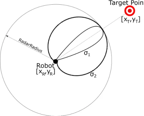
standard deviation and is a user-selectable parameter. Figure 7 shows two target distributions with two different values for σ.

Changing σT will impact the robot’s behavior. Smaller values will force the

(30)

Figure 7: Two target distributions with different σ values.

a greater higher turning radius around the obstacles, resulting in a safer trajectory with less risk of collision. However, a greater avoidance of the obstacles will result in a greater travel distance to the target, which will result in an increase in traveling time. BBO will be used to optimize the value forσT, as explained in the next chapter.

2.3 Obstacle Distribution dO

The obstacle distribution is constructed by the 360◦ radar sensor on the robot. The radar system was explained in section 2.1. The obstacle distribution dO is a function

of the distance sensed by the radar to the nearest obstacle at each angular position around the robot. The output of fθ in Equation 2.1 for input dO will return an

angle at which the robot has the lowest probability of colliding with an obstacle. In Section 2.1 it was explained that the radar distance array contains normalized values

(31)

for distance. We define the following equation for d0_O, which normalizes dO:

d0_O= dO

γ (2.7)

whereγis a coefficient that affects how sensitive the robot is to obstacles. If γis large the robot will be less sensitive. In our experiments, the value of γ is the maximum range of the radar, which results in

max(d0_O(φ)) = 1, φ∈[0,2π) (2.8)

The minimum value of dO is zero, which occurs when an obstacle is touching the

robot. In our experiments this happens rarely since the robot tends to move away from obstacles. In our experiments, this happens only if the speed of an obstacle is higher than that of the robot. In the following sections, the speed of the robot is discussed in more detail. There are some situations where the maximum speed of the robot is less than the speed of the obstacles, which could easily result in a collision. Figure 8 shows a sample obstacle distribution (d0) with maximum distance 1, which means there are no obstacles in that direction; these directions are indicated in the figure with the symbol B. If the distribution value is less than 1 in some direction, indicated with an A in the figure, an obstacle is detected within the radar range in that direction.

The simplest situation in simulation considers the robot as a point with zero radius. However, in the real world, the robot has a nonzero dimension. In order to establish a safe margin when the robot tries to go around the corner of an obstacle, we define a threshold JdF which shifts the obstacle distribution down. This means

the robot treats the obstacles as closer than their real positions. The value of this parameter is a function of the robot dimensions but is determined experimentally and is optimized later in this thesis.

(32)

Figure 8: Obstacle distribution d0. There are two types of regions in this figure: A indicates the existence of obstacles at the given angles, and B indicates that there are no obstacles at the given angles.

2.4 Final target distribution dF

The algorithm uses dT and d0O to construct the final target distribution dF,

which tells the robot which direction to choose to prevent colliding with obstacles while still moving as directly as possible toward the target. The algorithm constructs dF by taking the minimum value ofdT and d00 at each angle φ∈[0,2π):

dF(φ) = min(dT, d0O), φ ∈[0,2π) (2.9)

By using the minimum operation to construct the final target distribution, directions toward obstacles have a lower distribution value, and directions away from obstacles have a higher distribution value. The fθ function, described earlier, can be used to

find Θ, which is the argument of the maximum value of dF, which will be the most

favorable angle for a trajectory that is both safe and in the direction of the target point. Figure 9 shows an example of dF.

(33)

Figure 9: Example of final target distribution construction. The original target dis-tribution is green and the obstacle disdis-tribution is red. The solid line is the final target distribution and is constructed by taking the minimum value of the original target distribution and the obstacle distribution.

The robot also changes its speed depending on the location of the closest obstacle. Figure 10 depicts the speed algorithm of the robot. The robot has five speed modes: very slow (S1), slow (S2), normal (S3), fast(S4), and very fast (S5). The velocity of each speed mode will be optimized by the BBO algorithm. The robot changes its speed based on the location of the nearest obstacle according to Figure 10. In Figure 10, the robot is shown as a black filled circle in the middle of the figure, and the direction of motion is toward the top of the page and is shown with an arrow. The radius of the largest circle is L, which is the maximum range of the 360◦ radar. As the robot navigates and passes obstacles, some obstacles might enter the regions A,B,C, orD. If the closest obstacle is in regionA, the robot will choose speed mode S2. Region B is associated with speed mode S1, and regionsC, D, E, andF are associated with speed modesS5,S4,S3, andS3 respectively. If there is an obstacle in region E or F the robot will ignore them and will continue with normal speed S3. Region B is a symmetric arc with angle 2θ2 and is taken from a circle

(34)

centered on the robot with radius rB. Likewise, region C is a symmetric arc with

angle 360−2θ1 and is taken from a circle centered on the robot with radiusrC. rB and

rC are independent and belong to [0, L]. Parametersθ1, θ2,rB andrC are empirically

determined and highly affect the safety of the robot. They will be optimized later in this thesis with the BBO algorithm. The parameters are summarized in Table I.

Figure 10: Different speed mode regions that the robot uses to change its speed according to the position of the closest obstacle.

Location of closest obstacle Radius Speed mode

Region A L (radar range) S2 (Slow)

Region B rB S1 (Very Slow)

Region C rC S5 (Very Fast)

Region D L (radar range) S4 (Fast)

Region E L (radar range) S3 (Normal)

Region F L (radar range) S3 (Normal)

(35)

2.5 Memory Distribution dM

The final target distribution dF constructed in the previous section is highly

goal-oriented. In complex maps, like mazes or buildings with multiple rooms, the robot might not be able to reach the target without backtracking (that is, returning to regions or rooms that it has already visited). However, current global robot path planners require the robot to have a memory to store previously visited locations on the map. Building the map or reconstructing the map can also be implemented with our algorithm, but this is not our goal since we want to develop an algorithm that uses as little memory as possible. Our algorithm’s memory is a queue that can save up to 500 previously visited coordinates. When the number of time steps exceeds 500, the earliest elements are discarded. The robot uses this queue to escape rooms or corners in which it might become stuck. This allows the robot to escape rooms and to backtrack through previously visited regions. Figure 11 depicts the memory queue. Note that the number of memory blocks in the queue can be changed and can be optimized. However, in our simulations, the number of the blocks is constant and is equal to 500.

Figure 11: Memory queue in which previously visited coordinates are stored.

The robot saves the previously visited coordinates in memory as it navigates. These saved coordinates create a repulsive force. If the robot gets trapped in a room or a dead end, the memory points that are saved in that area become more dense. This will cause the robot to backtrack and escape from that area. The direction of the repulsive force follows a Gaussian distribution centered at the mean of directions of the memory points with standard deviation σM, which will be optimized later in

(36)

Figure 12 shows an example of the robot and the memory points (MPs) stored in the queue (fewer than 500 for the sake of illustration). Figure 13 shows a Gaussian distribution based on the MPs. As shown in Figure 13, the MP in the middle has the highest weight.

Figure 12: Illustration of memory points (MPs). The dashed lines show the direction of the repulsive force imparted to the robot by each MP.

Figure 13: Memory distribution based on recently visited locations.

The navigation algorithm executes at 60 Hertz, so the 500-point memory queue contains data for the previous 8 seconds, approximately. The distance traveled in 8

(37)

seconds depends on the speed of the robot. In a real-world application, 8 seconds might not be long enough for the memory queue and the size of the queue might need to be adjusted. Each memory block will occupy 8 bytes. As mentioned above, the robot uses 500 blocks for the queue, so the total memory requirement is 8 bytes×500 = 4000 bytes. This amount of memory is available in almost any embedded system. Table II compares the memory size required to store the coordinates of recently visited locations. This table shows that the required memory is appropriate even if we want to save 30 minutes worth of previously visited locations. However, the goal of this method is to keep the memory requirements as small as possible so that the algorithm is suitable even for small embedded systems.

Time Size 8 sec 3.75 KBytes 16 sec 7.5 KBytes 64 sec 30 KBytes 10 min 281.25 KBytes 30 min 843.75 KBytes 1 hour 1687.5 KBytes

Table II: Memory size comparison for various lengths of time for which the robot will save previously visited points. The nominal value in this thesis is 8 seconds.

2.6 Final Robot Steering Direction: Combining dM and dF

At this point we have steering angles from the memory distribution and the final target distribution. We call these steering angles VdF and VdM respectively.

In order to determine the final robot steering direction, the robot uses the memory vector only if necessary, so the memory vector has a lower weight than the final target vector on the final robot steering direction. To implement this idea, we assign weights to the two steering vectors: PdF for VdF, and PdM for VdM. The appropriate values

for the weights are determined empirically and in our experiments are optimized by BBO. The resultant vector is calculated by summing the two weighted VdF and VdM

(38)

vectors, and we call the resultant vectorVR. Figure 14 illustrates aVR calculation. In

the figure, VdF shows the final target steering direction as determined by the target

location and the obstacles, and VdM shows the steering direction as indicated by the

robot’s memory to avoid previously visited coordinates.

Figure 14: Illustration of dF and dM vectors and their weighted summation vector,

which is the final robot steering direction.

Figure 15 shows an example of how the speed changes with time as the robot navigates. The speed of the robot is changes between 4 and 10 units, since most of the time obstacles are detected in front of the robot so the robot slows down to avoid collisions. For the same simulation, Figure 16 shows how the distance to the target changes with time. If there were no obstacles on the map, the distance curve would be the dashed line in the figure. However, the obstacles make the robot veer from the straight path to avoid collisions.

(39)

Figure 15: Illustration of how the speed of the robot changes with time based on sensed obstacles.

Figure 16: Illustration of how the robot moves toward the target while avoiding obstacles.

(40)

CHAPTER III The D* ALGORITHM

The D* algorithm is based on the A* algorithm, which is a heuristic, robust, reliable path planning method that has been used in many applications [7,10,12]. The A* algorithm [27] searches for the best path through an environment by examining all possible paths from a known starting location to the known destination. A* considers a cost function like f(n) = g(n) +h(n) where n is the current graph number, f(n) is the cost to be minimized, g(n) is the cost from the starting graph to graph n, and h(n) is the heuristic that estimates the cost from graph n to the destination. One of the most ubiquitous path planning methods is D* [20, 32], or dynamic A*, which is a heuristic path planning method for dynamic environments. The D* algorithm is designed to plan the optimum trajectory for a robot as the robot moves through a map in real time. In this chapter, D* will be explained and compared to our newly proposed probabilistic method from the previous chapter.

3.1 Algorithm

The D* algorithm is a generalized version of A* and can be viewed as an attempt to find a sequence of state transitions through a graph. The graph node in our experiments is the position of a robot in some environment. The optimum path is the path, among all possible paths through the graph, for which the sum of transition costs is minimal. If any path through the graph is found to be not

(41)

optimal, the path is regenerated by the path planning algorithm. The cost of the robot states in the path can be defined as any measurable value, like distance, energy, time, etc. In the D* algorithm the robot uses a sensor to obtain information about the map. The map is partially known to the robot and the robot can re-plan its trajectory as it moves through the map. To generate the initial candidate optimum path, several methods have been published, such as the initial A* path and the distance-based initial path [24, 27]. In this research the distance-based initial path was implemented [24]. There are other methods that have been designed to improve the path of a robot in a graph based map, but they become highly inefficient in high resolution maps with a large number of graph nodes [2, 38]. D* provides an improvement over the previously mentioned algorithms because it can handle large maps by updating only the parts of the map that are required for the current steering decision of the robot.

D* works by first generating a path to the target point using the A* algorithm and begins moving toward the target point using that path. Figure 17 shows a map with the robot indicated with the green R and the target point with a red T. The gray areas are obstacles that are known prior by the robot. The arrows in the map show the steering directions generated by the A* algorithm. Note that the robot can move diagonally. If the robot follows the arrows, it will lead the robot to the target point. However, the tile indicated with O means that the robot is not aware if that tile is blocked or open. Based on the direction of the arrows, the robot will go between the obstacles and will arrive at the tile indicated with O.

D* has been extensively used in real robots [34]. D* star works by creating an OPEN list that includes two type of states: RAISE and LOWER. The RAISE states mean that the path cost will be increased and the LOWER states mean that the path cost will be reduced by redirecting the arrows to a new path. RAISE states increase the cost of each state by starting from a blocked state O and then sweeping outward

(42)

Figure 17: Sample tile map and A* navigation. The robot’s initial point is indicated with an R and the target point is indicated with a T. State O shows a tile in the graph whose state (open or closed) the robot does not know. Gray static obstacles are known to the robot prior to path planning. Arrows show the optimum path to the target point as computed by the A* algorithm based on prior knowledge of the map.

to activate the neighboring LOWER states. LOWER states compute the cost and change the direction of the arrows. D*, like A* [32], can use focused heuristics to achieve cost estimation that helps the robot arrive at its destination with a lower cost, less memory, and less computing power.

The D* algorithm consists of three main functions: PROCESS-STATE, MODIFY-COST and MOVE-ROBOT. PROCESS-STATE is the first step of the algorithm and finds

(43)

MODIFY-COST computes new cost values for different states. If there is a state with a high cost in the pre-computed path, this function puts the state in the OPEN list and maintains the RAISE and LOWER states of all affected states. In the last step, function MOVE-ROBOT causes the robot to move in the optimally defined direction. A detailed explanation of the D* algorithm is provided in [33].

In order to enhance the D* algorithm’s computational effort, it was modi-fied [19,21] using the lifelong planning A* algorithm to create a new algorithm called D* Lite. Although D* was implemented in this thesis, it was found to be compu-tationally inefficient so we instead use D* Lite, which will be explained later in this chapter.

3.2 Lifelong Planning A* (LPA*)

LPA* is an enhanced and incremental version of A* and applies A* to a finite graph whose edge costs increase or decrease over time. Algorithm 1 shows the LPA* algorithm. S indicates the finite set of vertices of the graph. Succ(s) ⊂S indicates the successors of the current vertex (s ∈ S) of the graph. Successors are vertices that are accessible and reachable from the current vertex. P red(s)⊂ S denotes the predecessors of the current vertex. Predecessors are vertices from which the current vertex (s∈S) can be reached. c(s, s0) represents the cost of moving from vertex sto vertex s0, s ∈ Succ(s). g∗(s) denotes the shortest path from sstart to s ∈ S. LPA*

always finds the shortest path between sstart and sgoal assuming knowledge of the

graph topology and costs. Like A*, LPA* uses heuristics, denoted as h(s, sgoal), to

approximate the distances to the goal vertex, where s∈S [34]. The heuristics should obey the triangle inequality:

h(sgoal, sgoal) = 0

h(s, sgoal)≤c(s, s0) +h(s0, sgoal)

(44)

Furthermore, the type of queue U will impact the behavior of the algorithm and is a priority queue. The LPA* functions are summarized in Table III.

Function Description

U.Top() Returns the vertex with the smallest priority in the queue U U.TopKey() Returns the smallest priority in the queue U

U.Pop() Returns the smallest priority in the queue U and deletes it U.Insert(s, k) Inserts vertex s in queue U and sets the priority to k U.Update(s, k) Updates the priority of vertex s in the queue U to k U.Remove(s) Removes vertex s from queueU

Table III: Functions of priority vertices queueU

If queueU is EMPTY the function U.TopKey(·) returns [∞,∞]. The variable rhs(s) in Algorithm 1 is defined as rhs(s) =        0, if s =sstart

mins0_∈_{P red}₍_s₎(g(s0) +c(s0, s)), otherwise

(3.2)

rhs(s) is function that looks ahead to obtain better information for g-values. LPA* estimates g(s) from the starting distance of the vertex s. LPA* g-values directly correspond to A* g-values.

Priorities in priority queue U are based on their key, k(s). The key of each vertex consists of two components:

k(s) = [k1(s)], k2(s)]

k1(s) = min(g(s), rhs(s)) +h(s, sgoal)

k2(s) = min(g(s), rhs(s))

(3.3)

where k1(s) corresponds to the f function of the A* algorithm f = g+h. LPA* g-values and rhs g-values correspond to A* g-g-values, and the LPA*hfunction corresponds to A* h-values. k2(s) corresponds to A* g-values. Keys are sorted by their first components, and if two keys have the same values in their first component then the

(45)

second component is compared. Vertices in priority queue U are expanded starting with the smallest key.

Algorithm 1Lifelong Planning A*

1: procedure CalculateKey(s)

2: return [min(g(s), rhs(s)) +h(s); min(g(s), rhs(s))] 3: end procedure

4: procedure Initialize

5: U =∅

6: for all s ∈S, rhs(s) =g(s) = ∞

7: rhs(sstart) = 0

8: U.Insert (sstart, [h(sstart); 0])

9: end procedure

10: procedure UpdateVertex(u)

11: if (u6=sstart) then

12: rhs(u) = mins0_∈_pred₍_u₎(g(s0) +c(s0, u))

13: end if

14: if (u∈U) then

15: U.Remove(u)

16: end if

17: if (g(u)6=rhs(u)) then

18: U.Insert(u, CalculateKey(u))

19: end if

20: end procedure

21: procedure _{ComputeShortestPath}

22: while (U.T opKey()< CalculateKey(sgoal) OR rhs(sgoal)6=g(sgoal))do

23: u=U.P op()

24: if (g(u)> rhs(u))then

25: g(u) =rhs(u)

26: for all (s∈Succ(u))do

27: UpdateVertex(s)

28: end for

29: else

30: g(u) =∞

31: for all (s∈Succ(u)S

U) do 32: UpdateVertex(s) 33: end for 34: end if 35: end while 36: end procedure 37: procedure Main(()) 38: Initialize() 39: while (True) do 40: ComputeShortestPath()

(46)

41: Wait for changes in edge costs

42: for all (Directed edges (u, v) with changed edge costs do

43: Update the edge cost c(u, v)

44: UpdateVertex(v)

45: end for

46: end while

47: end procedure

The LPA* algorithm was implemented in C++ for this thesis. This is required to implement D* Lite, which is described in the next section and which uses LPA* as an efficient part of its path planning algorithm.

3.3 D* Lite

In the previous section we described the LPA* algorithm. LPA* uses the edge costs of the graph to find the shortest path between the start vertex and the goal vertex. The D* algorithm uses the LPA* algorithm to find the shortest path as the robot navigates through a map. The D* algorithm is summarized in Algorithm 2. D* Lite is a path planning algorithm that can be used in unknown environments. For our experiments, the initial cost of each edge is 1. If there is no clear path to the goal vertex, the cost of the edges are set to infinity. In order to implement the D* Lite algorithm, the robot assumes that current location of the robot issstartand then

finds the path to sgoal.

Note that LPA* finds a path from sstart tosgoal, so the g-values are estimates

from the starting point. However, in D* Lite, the direction is reversed and the g-values are estimates from the goal point, so it finds the path from sgoal tosstart. To

address this issue in our research, when the map is not known but the immediate surroundings of the robot is known, the location of the start and goal vertices is exchanged in LPA*. Figure 18 shows the updated arrows as the robot navigates through the map. D* Lite is easier to implement and debug than the D* algorithm, and is claimed to be faster as well. So in this research, the D* Lite was implemented

(47)

and is compared to our newly proposed path planning method.

Algorithm 2D* Lite

1: procedure CalculateKey(s)

2: return [min(g(s), rhs(s)) +h(s); min(g(s), rhs(s))] 3: end procedure 4: procedure Initialize 5: U =∅ 6: km = 0 7: for all s ∈S, rhs(s) =g(s) = ∞ 8: rhs(sstart) = 0

9: U.Insert (sstart, [h(sstart); 0])

10: end procedure

11: procedure UpdateVertex(u)

12: if (u6=sgoal) then

13: rhs(u) = mins0_∈_Succ₍_u₎(g(s0) +c(s0, u))

14: end if

15: if (u∈U) then

16: U.Remove(u)

17: end if

18: if (g(u)6=rhs(u)) then

19: U.Insert(u, CalculateKey(u))

20: end if

21: end procedure

22: procedure ComputeShortestPath

23: while (U.T opKey()< CalculateKey(sstart)OR rhs(sstart)6=g(sstart)) do

24: kold=U.T opKey()

25: u=U.P op()

26: if (kold< CalculateKey(u))then

27: U.Insert(u, CalculateKey(u)) 28: else if g(u)> rhs(u)then

29: g(u) =rhs(u)

30: for all s∈P red(u) do

31: UpdateVertex(s)

32: end for

33: else

34: g(u) =∞

35: for all s∈P red(u)S

U do 36: UpdateVertex(s); 37: end for 38: end if 39: end while 40: end procedure 41: procedure Main 42: slast =sstart

(48)

43: Initialize()

44: ComputeShortestPath() 45: while sstart6=sgoal do

46: /* if (g(sstart) =∞) then there is no known path */

47: sstart=argmins0_∈_Succ₍_s

start(c(sstart, s

0_{) +}_g(s0₎₎ 48: Move to sstart

49: Scan graph for changed edge costs 50: if any edge costs changed then

51: km =km+h(slast, sstart)

52: slast =sstart

53: for all directed edges (u, v) with changed edge costsdo

54: Update the edge cost c(u, v)

55: U pdateV ertex(u) 56: end for 57: ComputeShortestP ath() 58: end if 59: end while 60: end procedure

Figure 18: An updated version of Figure 17 using D* Lite. The arrows have been been updated and the blocked gate between the two obstacles has been resolved.

(49)

3.4 Experimental Results

D* Lite is a graph-based path planner, so the resolution of the map is not perfect. In this section there is no optimization for either the probabilistic path planning algorithm or the D* Lite algorithm; the values of the parameters are chosen experimentally. The D* Lite algorithm was modified to include higher costs for vertices near obstacles so it could maintain some free space between the robot and the obstacles. There is no optimization involved in this set of comparisons. The number of time steps and number of collisions are recorded for both algorithms and are presented in this section.

The size of the map is 800×600 pixels. This corresponds to a map size of is 100 m× 75 m. In D* Lite the robot can see 80 pixels ahead and in the probabilistic method the robot can see 10 m ahead. The sizes of the dynamic obstacles are random and range between 56-80 pixels or 7-10 meters. The directions of their movements are random as well and they can move in any direction. The two algorithms are tested in this section on three maps as shown in Figure 19. Each algorithm was simulated three times per map because of the random sizes and movements of the obstacles, and the results are averaged. The resolution of the maps is 10 pixels. This means that the robot will jump 10 pixels per time step in both the D* Lite and probabilistic algorithms. The adaptive speed feature for the probabilistic method is disabled to provide a more even comparison.

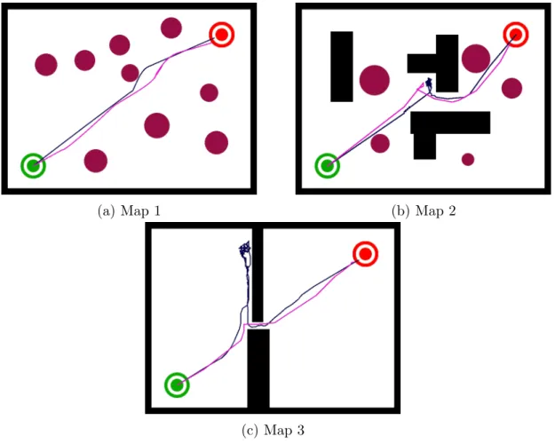
Map 1, shown in Figure 19a, contains only dynamic obstacles and no static obstacles except the surrounding walls. The blue line shows a sample path of the robot using the probabilistic approach and the red line shows a sample path using D* Lite. There are nine dynamic obstacles in the map and their direction of motion is random. We can observe that the robot paths for the two algorithms are similar. Both robots start moving toward the target point and change their paths to avoid the dynamic obstacles that appear in the visible radar radius. The speed of the dynamic obstacles

(50)

(a) Map 1 (b) Map 2

(c) Map 3

Figure 19: Maps used to compare the results for the probabilistic method and the D* Lite algorithm

are slightly higher than the robot, which makes occasional collisions inevitable. Map 2, shown in Figure 19b, constains both static and dynamic obstacles. The robots try to avoid both the static obstacles and the dynamic obstacles. However, the robot does not which obstacles are static and which ones are dynamic. The blue line shows a sample path for the probabilistic method and the red line shows a sample path for D* Lite. D* Lite spends less time than the probabilistic method finding the path to the target.

Map 3, shown in Figure 19c, shows an environment with only static obstacles. The robot needs to find the gap in the wall and successfully navigate through it. The blue line shows a sample path for the probabilistic method and the red line shows a sample path for D* Lite.

(51)

Table IV presents the overall comparison between the two algorithms. D* Lite had better results in terms of the time required to reach the target, but the probabilistic method resulted in fewer collisions. However, we should consider that the maps were converted to a grid of vertices to make this comparison. For larger maps, or for maps with higher resolution, the probabilistic method won’t have the performance penalty that D* Lite has, but D* Lite will take more time to reach the target point. D* Lite will also require more computing power as the number of nodes increases, while the probabilistic method requires computing power that is independent of the number of nodes. Overall, it appears that the probabilistic method is more suitable for real-world applications in which collisions are a primary consideration, and is a competitive path planning method for unknown environments with dynamic obstacles. In the next chapter the parameters of the robot are optimized using BBO.

D* Lite Probabilistic Method Map Collisions Time Step Collisions Time Step

Map 1 2.34 141.67 0.34 180

Map 2 1.34 171 1 211.34

Map 3 0 151 0 266.34

(52)

CHAPTER IV

BIOGEOGRAPHY-BASED OPTIMIZATION

Biography-based optimization (BBO) is an optimization algorithm based on the study of the geographical distribution of biological species. The study of bio-geography dates back to the 19th century [31] when scientists began analyzing the migration behaviors of species between islands and the reasons for their extinction. BBO applies the mathematics of biogeography to engineering problems.

There are many heuristic optimization methods, such as genetic algorithms (GAs), neural networks, fuzzy logic and particle swarm optimization. Due to the advantages of BBO, which will be discussed in the following, BBO is the method chosen in this research. As a general overview, habitat suitability index (HSI) is a metric of how suitable an island is for habitation. Habitats of an island with higher HSI tend to live longer and have a higher population than habitats in islands with a lower HSI. Because of this, the population of an island with a high HSI tends to emigrate to an island with a lower HSI. Figure 20 represents a map containing different islands with population members represented by gray dots. Representatives of these members tend to move to islands with lower HSI as discussed above.

In this research, we generate a population of islands where each individual has multiple parameters that define its characteristics. To measure the “goodness” of a member of the population, a cost function is defined. This cost function evaluates a metric for each member of the population so they can be compared to each other and

(53)

Figure 20: Biogeography migration of species to islands with lower habitat suitability index

sorted. Each iteration of the algorithm, a new population is generated via migration of parameters between members. However, a specific number of elite population members are maintained from the previous generation to prevent the loss of a good solutions to the underlying engineering problem. The number of elite members is empirical and affects how fast the algorithm converges to a population with optimized parameters.

Similar to biological species, in BBO an individual member of the population might mutate.The mutation probability is usually not high, but just as in biology a mutation might lead to an improved phenotype, in BBO mutation might lead to an improved member of the population. Mutation can also prevent the optimization process from getting stuck in a local optimum.

In our application, each member of the population includes a set of parameters to be optimized. Each parameter is initially randomly generated for each population member in the appropriate range. In a population of size n we begin BBO with n collections of randomly generated parameters. In our application, this corresponds to n robots, where each robot is simulated using its own unique set of parameters.

(54)

We define the variable T_ig to denote the number of time steps to reach the target and C_ig to denote the number of collisions in BBO generation g where i ∈ [1, n] is the index of the particular member of the population. However, note that a given robot simulation will not return the same T_ig and C_ig values because of the randomness of the simulations; the locations and movements of the dynamic obstacles are random and vary from one simulation to the next. To quantify the average performance of the path planning algorithm for a given set of path planning parameters, we use Monte-Carlo simulations for each robot:

T_ig = T g i1+T g i2+...+T g iM M i∈[1, n] C_ig = C g i1+C g i2+...+C g iM M i∈[1, n] (4.1)

where M is the number of the Monte-Carlo iterations, i indicates the index of a specific member of the BBO population, n is the population size and g is a specific BBO generation number.

The robots keep track of their values of T_ig and C_ig and save them in a file as soon as they reach the target point. Since we want to minimize both T_ig and C_ig, we consider a cost function which includes both. However, a lower number of collisions has a higher priority than the time to reach the target. Therefore, our first step is to sort the population based on T_ig and divide it into two sections based on an experimental thresholdQ. Then, all members that haveT_ig < Q, are sorted based on C_ig. In this way we obtain a list of members that are ordered starting from the best (lowest)C_ig, each of which has T_ig < Q. This process is depicted in Figure 21. In the next step we choose our elite BBO members and proceed to the next generation. This continues for a desired number of generations, or until we stop achieving significant improvements. Then the algorithm reports the best member of the final population as the solution to the optimization problem.