Graduate Theses, Dissertations, and Problem Reports
2019
Immunity-Based Framework for Autonomous Flight in
Immunity-Based Framework for Autonomous Flight in
GPS-Challenged Environment
Challenged Environment
Mohanad Al Nuaimi
Follow this and additional works at: https://researchrepository.wvu.edu/etd
Part of the Acoustics, Dynamics, and Controls Commons, Aeronautical Vehicles Commons, Computational Engineering Commons, Controls and Control Theory Commons, Navigation, Guidance, Control and Dynamics Commons, and the Robotics Commons
Recommended Citation Recommended Citation
Al Nuaimi, Mohanad, "Immunity-Based Framework for Autonomous Flight in GPS-Challenged Environment" (2019). Graduate Theses, Dissertations, and Problem Reports. 4081.
https://researchrepository.wvu.edu/etd/4081
This Dissertation is protected by copyright and/or related rights. It has been brought to you by the The Research Repository @ WVU with permission from the rights-holder(s). You are free to use this Dissertation in any way that is permitted by the copyright and related rights legislation that applies to your use. For other uses you must obtain permission from the rights-holder(s) directly, unless additional rights are indicated by a Creative Commons license in the record and/ or on the work itself. This Dissertation has been accepted for inclusion in WVU Graduate Theses, Dissertations, and Problem Reports collection by an authorized administrator of The Research Repository @ WVU. For more information, please contact [email protected].
Immunity-Based Framework for Autonomous Flight in
GPS-Challenged Environment
Mohanad Al Nuaimi
Dissertation submitted to the
Benjamin M. Statler College of Engineering and Mineral Resources at West Virginia University
In partial fulfillment of the requirements for the degree of
Doctor of Philosophy in
Aerospace Engineering
Mario Perhinschi, Ph.D., Chair Patrick Browning, Ph.D. Christopher Griffin, Ph.D.
Jason Gross, Ph.D. Majid Jaridi, Ph. D.
Department of Mechanical and Aerospace Engineering Morgantown, West Virginia
July 16, 2019
Keywords: Artificial Immune System, GPS-denied Environment, Autonomous Aerial Vehicle.
ABSTRACT
Immunity-based Framework for Autonomous Flight in GPS-denied Environment Mohanad Al Nuaimi
In this research, the artificial immune system (AIS) paradigm is used for the development of a conceptual framework for autonomous flight when vehicle position and velocity are not available from direct sources such as the global navigation satellite systems or external landmarks and systems. The AIS is expected to provide corrections of velocity and position estimations that are only based on the outputs of onboard inertial measurement units (IMU). The AIS comprises sets of artificial memory cells that simulate the function of memory T- and B-cells in the biological immune system of vertebrates. The innate immune system uses information about invading antigens and needed antibodies. This information is encoded and sorted by T- and B-cells. The immune system has an adaptive component that can accelerate and intensify the immune
response upon subsequent infection with the same antigen. The artificial memory cells attempt to mimic these characteristics for estimation error compensation and are constructed under normal conditions when all sensor systems function accurately, including those providing vehicle
position and velocity information. The artificial memory cells consist of two main components: a collection of instantaneous measurements of relevant vehicle features representing the antigen and a set of instantaneous estimation errors or correction features, representing the antibodies. The antigen characterizes the dynamics of the system and is assumed to be correlated with the required corrections of position and velocity estimation or antibodies. When the navigation source is unavailable, the currently measured vehicle features from the onboard sensors are matched against the AIS antigens and the corresponding corrections are extracted and used to adjust the position and velocity estimation algorithm and provide the corrected estimation as actual measurement feedback to the vehicle’s control system. The proposed framework is implemented and tested through simulation in two versions: with corrections applied to the output or the input of the estimation scheme. For both approaches, the vehicle feature or antigen sets include increments of body axes components of acceleration and angular rate. The correction feature or antibody sets include vehicle position and velocity and vehicle acceleration
adjustments, respectively. The impact on the performance of the proposed methodology
produced by essential elements such as path generation method, matching algorithm, feature set, and the IMU grade was investigated. The findings demonstrated that in all cases, the proposed methodology could significantly reduce the accumulation of dead reckoning errors and can become a viable solution in situations where direct accurate measurements and other sources of information are not available. The functionality of the proposed methodology and its promising outcomes were successfully illustrated using the West Virginia University unmanned aerial system simulation environment.
iii
Acknowledgment
I would like to sincerely thank my parents for supporting me throughout my life and showing the value of hard work and that any goal can be accomplished. I would also wish to thank my family and friends for their love and unforgettable support.
Most importantly, I thank my advisor Dr. Mario Perhinschi for his boundless patience,
invaluable advice, wisdom, guidance, support, and teachings throughout my education. Also, I thank my other committee members for their guidance and assistance.
iv
Table of Contents
List of Figures ... viii
List of Tables ... xii
Nomenclature ... xiv 1. Introduction ... 1 1.1. Motivation ... 1 1.2. Research Objective ... 2 1.3. Thesis Overview... 4 2. Literature Review ... 5 2.1 . Autonomous Trajectory Tracking ... 5
2.2. Bio-inspired Computational Techniques ... 6
2.2.1. The Genetic Algorithm ... 6
2.2.2. Ant-Hill Algorithms ... 6
2.2.3. Artificial Neural Networks ... 7
2.2.4. Fuzzy Logic ... 8
2.2.5. Particle Swarm Optimization ... 9
2.2.6. The Artificial Immune System ... 9
2.3. Global Navigation Satellite System ... 10
2.4. GNSS Vulnerability ... 11
2.4.1. Uncertainty Sources in GNSS ... 11
v
2.5. Inertial Measurement Unit (IMU) ... 13
3. General Formulation of the AIS-based Framework ... 15
3.1. The AIS Paradigm ... 15
3.2. Problem Formulation ... 16
3.3. Definitions and Notations ... 17
3.3.1. The Aircraft (or UAV) Reference Frame and Coordinate System ... 17
3.3.2. Earth Reference Frame and Coordinate System ... 18
3.3.3. Euler Angles ... 18 3.3.4. Transformation Matrix ... 19 3.3.5. Vector Derivative ... 20 3.3.6. Position Vector ... 20 3.3.7. Velocity Vector ... 20 3.3.8. Acceleration Vector ... 21 3.3.9. Angular Position... 21
3.3.10. Angular Velocity Vector ... 21
3.3.11. Angular Acceleration Vector... 22
3.3.12. Actual Values ... 22
3.3.13. Measured Values ... 23
3.3.14. Estimated Values ... 23
vi
3.3.16. Artificial Memory Cells ... 23
3.4. AIS-based Framework Architecture ... 24
3.4.1. The AIS Generation ... 24
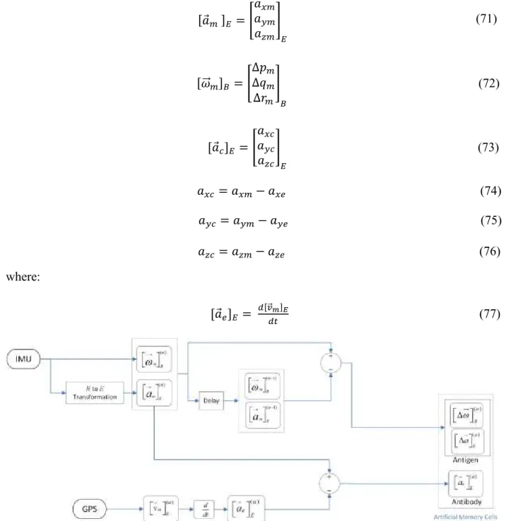
3.4.2. AIS Compensation ... 28
3.5. AIS Paradigm Challenges ... 30
4. The WVU UAS Simulation Environment ... 32
5. Example of Framework Implementation ... 34
5.1. Baseline Implementation ... 34
5.1.1. The UAV Features ... 34
5.1.2. The Acceleration and Angular Rate Measurements... 35
5.1.3. The Position and Velocity Estimation ... 35
5.1.4. The Correction Features ... 36
5.1.5. The Matching Algorithm ... 36
5.2. Correction of Estimation Scheme Output ... 37
5.2.1. AIS Generation... 37
5.2.2. AIS-based Estimation Correction ... 39
5.3. Correction of Estimation Scheme Input... 40
5.3.1. AIS Generation... 40
vii
6. Testing and Performance Evaluation ... 44
6.1. Experimental Design ... 44
6.2. Correction of Estimation Scheme Output ... 45
6.3. Correction of Estimation Scheme Input... 52
6.4. Effect of Navigation Accuracy on AIS... 56
6.5. Path Planning Comparison ... 59
6.6. IMU Grade Consideration... 61
6.7. Affinity Methods Comparison ... 63
6.8. UAV Features Analysis ... 64
6.9. Augmentation of Position and Velocity Vertical Components... 68
7. Conclusion ... 71
viii
List of Figures
Figure 1. Immunity cell interactions. ... 16
Figure 2. The aircraft reference frame. ... 17
Figure 3. Earth reference frame. ... 18
Figure 4. Roll, pitch, and yaw rotation axes. ... 19
Figure 5. Building the AIS (off-line). ... 25
Figure 6. Estimation scheme and processing corrections for the “output” approach. ... 26
Figure 7. Estimation scheme and processing corrections for the “input” approach. ... 26
Figure 8. On-line AIS compensation. ... 29
Figure 9. Correction of the output of the estimation scheme ... 29
Figure 10. Correction of the input of the estimation scheme. ... 30
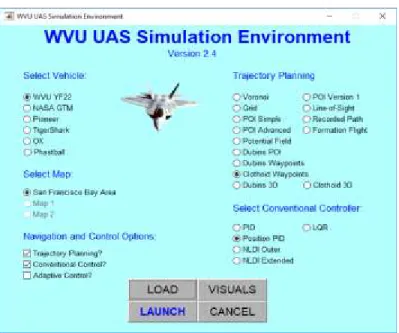
Figure 11. WVU UAS simulation figure environment mission scenario setup menu. ... 32
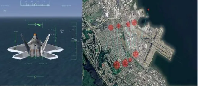
Figure 12. WVU UAS simulation environment–visualization interfaces. ... 33
Figure 13. Errors model for the IMU components (accelerometer and gyroscope). ... 33
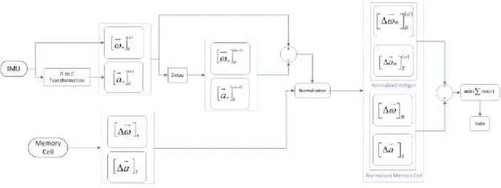
Figure 14. Immune affinity for antibody extraction. ... 37
Figure 15. Generating AIS as a collection of artificial memory cells including antibodies of velocity and position. ... 39
ix
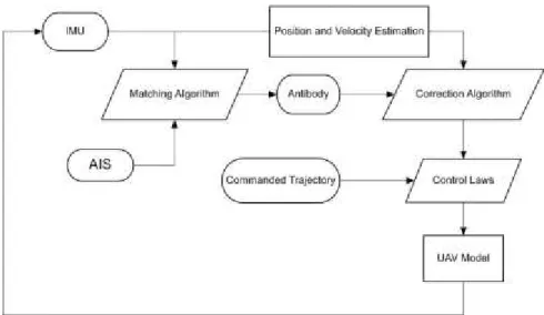
Figure 17. Closed loop UAV system with AIS correction of position and velocity. ... 40
Figure 18. Generating AIS as a collection of artificial memory cells including antibodies of acceleration. ... 42
Figure 19. Correction of the acceleration components. ... 43
Figure 20. Closed loop UAV system with AIS correction of acceleration. ... 43
Figure 21. AIS generation trajectory #1. ... 46
Figure 22.AIS generation trajectory #2. ... 46
Figure 23. AIS generation trajectory #3. ... 46
Figure 24. AIS generation trajectory #4. ... 46
Figure 25. AIS generation trajectory #5. ... 46
Figure 26. AIS generation trajectory #6. ... 46
Figure 27. Tracking of AIS generation trajectory under nominal conditions scenario. ... 48
Figure 28. Tracking of validation trajectory #1 under nominal conditions scenario. ... 48
Figure 29. Tracking of AIS generation trajectory with estimation scheme only. ... 48
Figure 30. Tracking of validation trajectory #1 with estimation scheme only. ... 48
Figure 31. Tracking of AIS generation trajectory with AIS corrected estimation... 49
Figure 32. Tracking of validation trajectory #1 with AIS corrected estimation. ... 49
Figure 33. Tracking of validation trajectory #2 under nominal conditions scenario. ... 49
x
Figure 35. Tracking of validation trajectory #2 with estimation scheme only. ... 49
Figure 36. Normalized tracking errors of AIS generation trajectory. ... 50
Figure 37. Normalized tracking errors of validation trajectory #1. ... 50
Figure 38. Normalized errors of validation trajectory #2. ... 50
Figure 39. Nominal generation trajectory. ... 53
Figure 40. Estimation scheme generation trajectory... 53
Figure 41. AIS generation trajectory. ... 54
Figure 42. AIS first validation trajectory. ... 54
Figure 43. AIS second validation trajectory. ... 54
Figure 44. Normalized tracking errors of generation trajectory. ... 54
Figure 45. Normalized tracking errors of first validation trajectory. ... 55
Figure 46. Normalized errors of second validation trajectory. ... 55
Figure 47. Perfect nominal errors. ... 58
Figure 48. GPS nominal errors. ... 58
Figure 49. Effect of GPS on errors. ... 59
Figure 50. Dubins and clothoid trajectories AIS comparison without estimation. ... 60
Figure 51. Dubins and clothoid trajectories AIS comparison with estimation. ... 60
xi
Figure 53. Effect of IMU grade on AIS ... 62
Figure 54. Normalized tracking errors for different affinity methods. ... 63
Figure 55. Determination of UAV features effect on matching algorithm. ... 65
Figure 56. UAV features matching accuracy. ... 65
Figure 57. Weighted mismatching of UAV features. ... 66
Figure 58. Effect of including the angular acceleration on the matching accuracy. ... 67
Figure 59. Effect of 𝜔 features on the AIS performance. ... 68
Figure 60. Vertical components compensation. ... 69
Figure 61. Generation trajectory #1 normalized errors. ... 70
Figure 62. Generation trajectory #1 normalized errors with estimation. ... 70
Figure 63. Validation trajectory #1 normalized errors... 70
xii
List of Tables
Table 1. The percentage improvement of trajectory tracking under the AIS scenario. ... 51
Table 2. Percentage change in errors for AIS generation trajectory with respect to nominal errors. ... 51
Table 3. Percentage change in errors for validation trajectory #1 with respect to nominal errors. ... 51
Table 4. Percentage change in errors for validation trajectory #2 with respect to nominal errors. ... 51
Table 5. The AIS percentage improvement. ... 55
Table 6. Percentage change in errors for generation trajectory with respect to nominal errors. .. 56
Table 7. Percentage change in errors for validation trajectory #1 with respect to nominal errors. ... 56
Table 8. Percentage change in errors for validation trajectory #2 with respect to nominal errors. ... 56
Table 9. Effect of GPS on errors. ... 58
Table 10. clothoid errors comparison ... 61
Table 11. Dubins errors comparison ... 61
Table 12. IMU grades. ... 62
Table 13. Trajectory tracking errors of AIS for intermediate and aviation IMU grades. ... 63
xiii
Table 15. Effect of angular acceleration and angular rate on AIS generation trajectory. ... 67
Table 16. Effect of angular acceleration and angular rate on AIS validation trajectory. ... 67
Table 17. Performance metrics comparison without using vertical component sensor
augmentation. ... 69
Table 18. Performance metric comparison with vertical component sensor augmentation. ... 70
xiv
Nomenclature
VARIABLES
Symbol Description Units
English 𝒆 Errors - 𝓕 Correction algorithm - 𝑫 Affinity distance - 𝒌 Time sample s 𝑳 Transformation matrix - 𝑴𝒋 Memory cell - 𝑵 Population size -
𝒑 Roll rate rad/s
𝒒 Pitch rate rad/s
𝒓 Yaw rate rad/s
𝒑⃗⃗ 𝟏 Position vector m 𝒗 ⃗⃗ Velocity vector m/s 𝒂 ⃗⃗ Acceleration vector m/s2 Greek 𝜶 Time sample s
𝜽 Pitch angle rad
𝝋 Bank angle rad
𝝋 AIS feature -
𝝍 Heading angle rad
𝝎⃗⃗⃗ 𝟏𝟏 Angular velocity vector rad/s 𝝎̇⃗⃗⃗ 𝟏𝟏 Angular acceleration vector rad/s2
∑𝟏 Summation
xv
ACRONYMS
Symbol Description
AI Artificial Intelligence
AIS Artificial Immune System
AMC Artificial Memory Cells
ANN Artificial Neural Network
CS Coordinate System
CSB Body Coordinate System
CSE Earth Coordinate System
DOP Dilution of Precision
GA Genetic Algorithm
GPS Global Positioning System
GNSS Global Navigation Satellite System
IMU Inertial Measurement Unit
MEMS Micro-Electric-Mechanical System
NNSS Navy Navigation Satellite System
NAVSTAR Navigation System with Timing and Ranging
PSO Particle Swarm Optimization
RF Reference Frame
RFB Body Reference Frame
RBF Radial Basis Functions
TOA Time of Arrival
UAG Unmanned Ground Vehicle
UAS Unmanned Aerial System
UAV Unmanned Aerial Vehicle
UD Upper Matrix and Diagonal Matrix
UKF Unscented Kalman Filter
1.
Introduction
1.1.MotivationThe demand for unmanned aerial vehicles (UAVs) has significantly increased due to their benefits and adaptability [1, 2]. UAVs are inexpensive, unmanned, lightweight, versatile, and capable of long endurance, which makes them desirable for use in many fields such as
reconnaissance, combat, surveillance, and payload delivery [3]. Safety is a primary concern for all flyable objects. In particular, using the UAVs in an urban areas has numerous limitations due to their safety issues [4]. The autonomous UAVs usually use a global navigation satellite system (GNSS) such as the global positioning system (GPS) to navigate unfamiliar urban and non-urban areas. However, GPS signals can be blocked or severely disturbed, limiting the capability of the system to deliver the required level of availability, accuracy, and reliability of positioning, thus, significantly affecting operational safety [5]. Also, the GPS could be affected by jamming, spoofing, and other technical issues [6]. Introduction of new alternative navigation methods is essential when the GPS is absent, ineffective, or too risky to be used.
Many elements are involved in the operation of autonomous UAVs. Generating the best
flyable trajectory of the UAV’s path of mission and tracking this trajectory is significantly essential to fulfill the UAV’s missions [7]. The trajectory tracking algorithms are expected to follow a commanded trajectory, while minimizing tracking errors. The commanded trajectory path planning can be initiated using a start and finish position, and velocity, waypoints, and obstacles. Al Nuaimi provided a detailed comparison between two methods of path planning [8]. Tracking the path of any moving or flying autonomous vehicle can be achieved using a GNSS [9], which provides feedback of the current position and velocity to a controller that adjusts the speed and the dynamic motion to update the position and velocity [10, 11].
The satellite navigation systems calculate the position of an object relative to known satellites’ positions within the Earth, with the satellite signal having the ability to cover a wide area over the globe [12]. The current position and velocity of autonomous vehicles are typically defined using the GNSS. However, reliable alternative solutions that provide similar accuracy and coverage as the satellite navigation systems are needed [13, 14]. Developing an autonomous aerial vehicle that can track the commanded trajectory when the GNSS signal is blocked or inefficient is a challenging objective [15].
The most widely used approach is based on additional information of opportunity, including landmarks that are identified using visual aids and image processing [16]. These methods are inefficient when the mapped area is changing, becomes dark, or is unclear due to environmental effects [16]. Watson and Gross [17] used the factor graph method of Simultaneous Localization and Mapping in conjunction with several robust optimization techniques to evaluate their applicability to robust GNSS data processing. Other methods involve the use of moving and fixed objects with known positions and velocity as a reference to determine the vehicle’s position and velocity. The limitation of these methods is that they are expensive and not always feasible [18]. In [19] and [20], Sivaneri and Gross investigated the cooperation between unmanned ground vehicles (UGVs) and UAV for navigation in a GNSS-challenged environment. The focus was on the design of the optimal motion of UGVs to best augment the solution of UAV
navigation.
Theoretically, a combination of accelerometers and gyroscopes or inertial measurement unit (IMU) can be used to measure the acceleration and orientation of moving objects. The integral of measured acceleration is used to estimate position and velocity; however, this approach may result in significant biases and large drifts [21]. This dissertation involved the investigation and proposition of a novel approach for correcting position and velocity estimates for autonomous flight vehicles when GPS information and other substitutes are not available based on the artificial immune system (AIS) paradigm.
1.2.Research Objective
The purpose of this research was to investigate the potential of and develop an AIS-based framework for the autonomous tracking of flight trajectories in a GNSS-challenged environment. The developed methodology is implemented and tested through simulation using the West Virginia University (WVU) unmanned aerial system (UAS) simulation environment [22]. The AIS paradigm [23] is inspired by mechanisms of the biological immune system of superior vertebrates which is capable of detecting and counteracting intruding exogenous entities (antigens) while overlooking the self cells [24]. The AIS paradigm exhibits highly robust and adaptive classification and information structuring capabilities, as well as memory and information fusion potential [25].
All these characteristics are beneficial in solving challenging technical problems such as autonomous trajectory tracking when GNSS information is not available. Mechanisms of the biological immune system are mimicked to compensate for the drifting error from integrated acceleration and obtain adequate position and velocity estimates. The general feasibility,
applicability conditions, constraints, and benefits of the proposed methodology were analyzed. In this research, a general AIS based framework was formulated to correct the inertial sensor
outputs. The AIS classification and memory capabilities were extended and used for autonomous flight control purposes.
The AIS can significantly mitigate the accumulating errors of the inertial sensors output caused by the integration of acceleration components. The AIS can be used not only with known trajectories that were used to build the AIS but also with new different trajectories. The AIS navigation methodology does not require supporting infrastructure, landmarks, or image
processing capabilities. The construction of the AIS requires extensive data that can be acquired before the mission at times and locations when vehicle position and velocity information is available.
The AIS paradigm is used for the first time in this context for UAV flight in GPS- challenged environment. The AIS paradigm represents a significant step towards developing a comprehensive and integrated solution for monitoring and controlling aerospace systems, including navigation and trajectory tracking. Note that these sets of data must be representative and complete in defining targeted system operational envelope.
A novel structure is developed and tested extensively for UAV trajectory tracking based on principles of artificial immune systems and used to analyze the effectiveness and performance of the proposed immunity-based framework. Two approaches for the proposed method were developed: 1) correction of the estimation scheme input, and 2) correction of the estimation scheme output. The artificial immune system was built with different trajectories and tested using generation and validation trajectories. The effect of path planning algorithm for the commanded trajectory, model of the affinity method, class of the selected sensors, selected features for the matching algorithm, and scenario when an external source of the vertical components’ measurements is available on the proposed method were investigated.
1.3.Thesis Overview
Chapter 1 has provided a comprehensive overview of the introduction and objectives of the dissertation. Chapter 2 presents a literature review of the autonomous trajectory tracking and bio-inspired techniques used to solve it, followed by a discussion of the global navigation
satellite system and its vulnerabilities. In addition, Chapter 2 provides a discussion of the inertial measurement unit and the source and modeling of its errors. Chapter 3 provides an overview of the general formulation of the AIS-based framework for autonomous trajectory tracking in GNSS challenged environments. Additionally, Chapter 3 describes the AIS paradigm, the problem formulation, definitions and notations, AIS-based framework architecture, AIS paradigm challenges, and the AIS generation. Chapter 4 provides an overview of the UAV simulation environment used to build and test the AIS framework. Chapter 5 provides an example of using and implementing the proposed AIS framework in two different tactics; one based on correcting the estimation output and the other based on correcting the estimation input. The matching algorithm and affinity techniques are also discussed in Chapter 5. Testing results and their analysis are presented in Chapter 6. Finally, Chapter 7 presents the conclusions of the dissertation based on the findings.
2.
Literature Review
2.1.Autonomous Trajectory TrackingThe capability of a system to accomplish tasks and missions without direct input from human operators is known as autonomy [26]. Autonomy implies that the system must possess characteristics of intelligence such as making decisions, performing self-configuration and optimization, sensing and evaluating the system status, and external context [27]. The most critical aspects of autonomous flight are adequate commanded trajectory generation, adjustment and modification, and high-performance control laws for trajectory tracking [28]. Given that following the commanded trajectory is the ultimate objective of autonomous flight, the position, and velocity of the vehicle in the inertial frame are critical. Three large classes of methods have been used individually or as a combination to determine the velocity and position of vehicles: Methods based on on-board sensors that can determine the relative vehicle location based on a known position of the initial point, those based on external sensors such as GNSS, and strategies utilizing on-board sensors capable of detecting or estimating relative vehicle position with respect to landmarks with a priori known locations [2].
The GNSS-based approach has become an effective solution because of its reliability and low cost. However, alternative approaches must be developed to be used as a substitution in the numerous situations when the GNSS is unavailable, not functioning correctly, or undesirable for use. An autonomous trajectory tracking and obstacle avoidance navigation system in GPS denied, and the cluttered environment was developed by Mohta et al. [29] using visual sensors. The navigation system consists of a set of integrated modules that work together to allow a quadrotor robot to move from a starting position to a specified location. Sensor fusion was applied to cameras, IMU, and lidar with unscented Kalman filter to determine position and velocity. Software architecture for safe and reliable autonomous navigation of aerial robots in GPS-denied areas was presented by Perez Grau [18] using a six-dimensional approach for localization and state estimation. Visual odometry and Monte Carlo localization were used for motion planning. Dead reckoning represents a class of algorithms that use inertial sensor measurements to obtain integration changes in position or velocity [30]. Zhou et al applied the dead-reckoning and discrete Kalman filter with the method of analytic geometry to improve the trajectory tracking accuracy of an unmanned quadrotor [31].
2.2.Bio-inspired Computational Techniques
Bio-inspired techniques result from the transfer of ideas, concepts, mechanisms, or general knowledge from the biological world into technical applications. The development and use of such approaches have remarkably increased over the last few decades in part due to the advent of powerful computers that made the associated substantial computational effort
affordable [32]. Before the computers were invented, biological systems solved similar complex problems for a long time, and with the availability of powerful computational tools today, tapping into this source of inspiration is possible and promising.
2.2.1. The Genetic Algorithm
John Holland and colleagues developed the Genetic Algorithm (GA) concept in the 1960s and 1970s [33]. The GA is a biological evolution model based on Charles Darwin’s natural selection theory. Studies using GAs have significantly increased in many fields, including adaptive agents in economic theory and design of sophisticated devices such as aircraft turbines and integrated circuits [34]. Nikolos [35] used a combination of a modified breeder GAs
incorporated with characteristics of classic ones to create an evolutionary-based framework to design an offline/online path planning for UAVs autonomous navigation. The path planner was used in a three-dimensional environment to calculate the path with curvature in rough terrain. An alternative way of position localization of quadrotor without using GPS or cameras was
presented by Faelden et al. [36]. The method was dependent on using a transceiver’s signal as inputs for the genetic algorithm to locate the quadrotor in x, y, and z-axis. Wilburn et al. [37] used a modified GA for gain optimizing of trajectory-tracking controllers for autonomous aircraft which facilitates the investigation of novel control architectures regardless of complexity and dimensionality.
2.2.2. Ant-Hill Algorithms
The ant colony algorithm is a technique for obtaining the optimal path which is compared to an ant’s behavior when searching for food. The complex social behavior of ants when
navigating in search of food sources using identical traffic paths (or ant streets) has drawn the attention of scientists[38]. Ants are animals with low-resolution vision [39] who can find the shortest routes between the feeding sources and their colony by repeatedly marking their paths with pheromones[40]. Initially, the ants choose random paths to the food source and mark them
with pheromone deposits. The ants who take the shortest path arrive at the food source and back at the nest faster than the others who take longer paths; meaning that a higher amount of
pheromone will be deposited on the shortest path as oppossed to the other paths. Because this path has the highest pheromone concentration, other ants will select it, and also deposit more pheromone causing even more concentration. Therefore, the shortest path is the optimal selected path to the food source [38]. The first attempt of the ant algorithm approach was in the early ‘90s
by Dorigo and colleagues [40]. The new approach uses a combination of distributed
computation, positive feedback, and a constructive greedy heuristic for stochastic optimization and problem-solving. Dorigo applied his approach to the classical traveling salesman problem with the results showing that the system can rapidly provide adequate solutions. A hybrid improvement strategy for the basic ant colony algorithm model was proposed by Ma and colleagues [41] for UAV optimal trajectory planning in a complex environment. The proposed method shows better performance than the basic ant colony algorithm in convergence speed, solution variation, dynamic convergence behavior, and computational efficiency.
2.2.3. Artificial Neural Networks
One of the unusual sources of inspiration for soft computing techniques is how the human brain works. The functionality of the human brain relies on many specialized cells interacting together within a highly interconnected system called a neural network. The Artificial Neural Network (ANN) is a learning-based computing technique based on information processing inspired by the brain’s biological neural network [42]. The ANN attempts to mimic the way information is processed by the brain. The first attempt of developing an ANN was by
McCulloch and Pittman in 1943 who published a simple neural network model using electrical circuits to describe how neurons in the brain work [43]. Since then, ANNs have been used successfully as general powerful function approximators or model generators for solving various technical problems. The reliability of the UAV navigation information when the environment characteristics change was improved by Guan and Cai [44] using an ANN based on Radial Basis Functions (RBF) with Kalman filter and particle filter. The filters used for data fusion and the RBF neural network were used to estimate the error of the particle filter. When the data are available, the neural network performs the training mode, and when the data flow is interrupted or unreliable, the system uses the trained model. The accuracy of the position in two dimensions
(x and y) has been significantly increased. The AIS paradigm augmented with artificial neural networks was used by Perhinschi and colleagues [45] for developing and testing through simulation aircraft sub-system failure detection and identification schemes. The AIS paradigm included the neural estimates of the angular accelerations defined as features affected by abnormal conditions.
2.2.4. Fuzzy Logic
Fuzzy logic is an alternative generalized logic that uses continuous truth values between 0 and 1 instead of only using the binary extremes. The fuzzy logic was first introduced by Lotfi Zadeh, a professor at the University of California at Berkley. In 1965, Zadeh published his first
paper on fuzzy logic entitled “Fuzzy Sets,’’ which was the beginning of numerous applications
of the fuzzy logic concept [46]. In 1973,Zadeh published another paper on the analysis of complex systems and decision processes and, in 1979, proposed the extensions of the possibility theory to the fuzzy information granules [47]. In 1981, Zadeh published another paper on possibility theory and soft data analysis [48].
Typically, the inputs of the fuzzy logic-based system are converted into outputs in three main steps: fuzzification, decision making, and defuzzification. Trajectory tracking for an autonomous UAV using fuzzy logic has been investigated by Perhinschi [49]. Sabo and Kelly developed a two-dimensional motion planning approach for a UAV using fuzzy logic to command the changes in heading angle and the speed [50]. The information about the target location and obstacles was sent to the fuzzy inference system in real time within the sensing range of the sensors. Sun et al. [51] examined path tracking and obstacle avoidance using a fuzzy logic approach. Moving and immobile obstacles were considered along with the preplanned path at each instant. Wilburn et al. demonstrated that a fuzzy logic-based scheme for UAV navigation possesses better capabilities compared to a potential field controller [52].
2.2.5. Particle Swarm Optimization
Particle Swarm Optimization (PSO) is a computational stochastic optimizing technique that attempts to iteratively improve a candidate’s solution with respect to a given measure of quality [53]. PSO was introduced in 1995 by Kennedy and Eberhart [54] as an optimization method to solve nonlinear problems. The PSO was inspired by the social behavior of certain bird and fish species that can coordinate the movements of many individuals quickly and accurately. PSO involves seeking the best solution in the search space. Each solution is called a particle and has a cost value that is minimized by the evaluation function. Ahmad Zadeh and Ghanavati proposed an approach for using PSO in mobile robot navigation in a dynamic environment [55]. The proper path to the goal position consisted of several points that were selected individually using the PSO optimization technique. Sensors were used to detect moving and fixed obstacles with a limited surrounding radius to successfully minimize the traveling time and distance, while avoiding obstacles.
2.2.6. The Artificial Immune System
Artificial Intelligence (AI) has proven its feasibility in many fields. Artificial intelligence techniques are inspired by various biological systems such as the immune system in superior vertebrates, which provided the ideas for the formulation of the AIS paradigm. Some of the most popular immunity concepts include the negative and positive selection algorithms, cloning and clonal selection, cellular memory, immune network theory, and danger theory. The general AIS methodology for system abnormal condition detection and identification was outlined by Dasgupta [56] including the highly robust ability of the organisms to detect, identify, and eliminate invading pathogens while overlooking its own cells.
The use of immune systems was primarily targeted at the detection and identification of the systems of abnormal and failure conditions. An AIS-based framework for aircraft abnormal condition detection, identification, evaluation, and accommodation was formulated by WVU researchers [57, 58]. The proposed methodology has the capability of providing an integrated and comprehensive solution to the problem of aircraft monitoring and control under normal and abnormal operational conditions [59]. Specific immunity-inspired approaches for abnormal condition detection, identification, evaluation, and accommodation have been developed. In particular, mimicking the capability of the immune system to memorize antigen/antibody
correlation was investigated with promising results for aircraft control purposes [60]. The immunity-based monitoring approach was successfully tested with actual UAV flight data [61] and hardware-in-the-loop simulation [62, 63]. Navigation and obstacle avoidance for a mobile ground robot was approached by Ozcelik and Sukumaran [64] using AIS; the obstacle’s position was assimilated to antigens and the required vehicle heading for adequate obstacle avoidance to the antibodies.
2.3.Global Navigation Satellite System
The United Nations defined the GNSS at the Third United Nations Conference on the Exploration and Peaceful Uses of Outer Space in 1998 as follows: “The Global Navigation Satellite System (GNSS) is a space-based radio positioning system that includes one or more satellite constellations, augmented to support the intended operation. The GNSS provides 24-hour three-dimensional position, velocity, and time information to suitably equipped users anywhere on or near the surface of the Earth (and sometimes off Earth)” [65].
The US military conceived the Navy Navigation Satellite System (NNSS) concept in the late 1950s and developed it in 1960s mainly for determining the time and coordinates of vessels at sea and military application on land. Eventually, the NNSS became authorized for civilian uses such as navigation and surveying. The US military later overcame the shortcomings of the early navigation systems and developed the Navigation System with Timing and Ranging (NAVSTAR) or GPS. The Russian military developed its counterpart to GPS, the Global Navigation Satellite System (GLONASS) while European countries also contributed to the GNSS with Galileo. Finally, the Chinese GNSS called BeiDou (Compass) is the first-generation regional system [65]. The principle of GNSS is based on a trigonometry solution of a
geometrical problem to determine positions using Earth stations as reference points. The receiver is located at the intersection of four spheres; each centered at known coordinates of the satellite that broadcast information to the receiver [12]. The pseudorange of each satellite defines the surface of a sphere with its center at the satellite position [65]. The radius of each sphere represents the distance between the satellite and the receiver or the
pseudorange. Three satellites are needed to measure the latitude, longitude, and height which can be determined using three range equations; however, there is an offset between the receiver’s
receiver. Therefore, a fourth satellite is needed to solve the four unknowns, namely three components of position plus the clock bias [65]. An integrated GNSS and vision sensor suite approach was used by Roberts [66] for aircraft collision and obstacle avoidance and navigation. The GNSS contribution was used to provide primary aircraft navigation, and the vision sensor was to provide obstacle and aircraft collision avoidance. Cho et al. [67] assumed that the inertial sensors such as gyros and accelerometers were disabled in a UAV and single-antenna GPS receiver based attitude determination system was used for fully automatic control of taxiing, landing, and take off on the runway for UAV. The single-antenna GPS receiver can be used as a primary sensor for a backup or a low-cost control system of UAVs.
2.4.GNSS Vulnerability
The distances between satellites and receiver or pseudoranges are calculated using the Time of Arrival (TOA) concept. TOA refers to the time it takes the electromagnetic wave signal of the satellite to propagate and reach the receiver within the shortest straight path. In other words, TOA measures the differences between the satellite and receiver clock times when the signal arrives at the receiver. The measured TOAs for each satellite multiplied by the speed of light to calculate the pseudoranges which are used in trigonometrical equations to calculate the user position [12]. Ideally, the satellite signal propagates in a vacuumed surrounding at a speed of light in an obstacle-free path without interferences, hardware faults and failures, and the clocks of the satellites and receiver are precisely synchronized. Any alteration to the ideal scenario causes errors and contributes to inaccurate user position [68]. In standard stand-alone operations of GNSS, TOAs provide a three-dimensional position of approximately 5-10 meters accuracy depending on user equipment infrastructure, error sources, and configuration for tracking.
2.4.1. Uncertainty Sources in GNSS
The GNSS signals are transmitted through different layers of the atmosphere such as the ionosphere and troposphere. These transmission media cause deviations of the traveling signal from the shortest path, increasing the travel time and causing position calculation errors [69]. The GNSS is affected by the ionospheric storms over the Equator; therefore, augmentation systems have been developed to make corrections to the message transmitted to user receivers [70]. For military uses, GPS signals are transmitted at two different frequencies to mitigate the ionospheric effect. Unfortunately, this service is not available for commercial non-authorized
users. However, several strategies such as using mathematical models and using additional information provided by ground, and space-based augmentations can be used to mitigate the ionospheric effect [71]. The troposphere ranges from the Earth surface to 17–20 km in altitude, whereas the ionosphere lies between 75 and 500 km. The difference between the expected and actual orbital position of a GNSS satellite determines the ephemeris errors, which create about a few meters of error in computing position. The geometric arrangement of satellites, as they are
“visible” to the receiver, affects the measurement through Dilution of Precision (DOP), which is a metric of geometric diversity of the satellites and relates parameters of the user position and time bias errors to those of the pseudorange errors. The DOP contributes to navigation accuracy and proper measurements can be obtained if adequate user/satellite geometry exists [12].
Receivers are designed to use signals from available satellites in a manner that minimizes this effect. Errors due to DOP are caused by poor positioning of satellites; thus, proper distribution of satellites produces better navigation [12]. If signals arrive over two or more paths due to multiple reflections, interferences in the receiver occur and affect the signal quality. Another cause of interfering is the weak signal from the satellite.
2.4.2. Radio Frequency Interference in GNSS
The GNSS satellites broadcast signals in two or more frequencies in L band, and typically these signals are received at low power on the Earth’s surface [72]. These signals can be disrupted by other Radio Frequency (RF) signals that appear in the bands. The interfering signals come intentionally or unintentionally from transmitting devices, causing poor GNSS receiver performance [6]; therefore, the receiver needs to detect these interferences to preserve adequate performance. The GNSS receivers can be interfered unintentionally by malfunctioning radio devices when they operate at the subharmonics of GNSS carrier frequencies [6]. The intentional interference is caused by devices intended to disrupt the normal GNSS operation and is referred to as jamming, spoofing, and meaconing [65]. Jamming involves transmitting a high-power signal close to the GNSS signal by jammer devices to mask it out and disable it from properly entering the receiver. Spoofing refers to a counterfeit signal that tricks the GNSS receivers to produce faulty information [12]. Spoofing is more challenging than jamming because the faked signal attempts to mimic a valid one and typically cannot be detected until a severe problem occurs, whereas the loss of signal caused by jamming is more apparent [73].
Meaconing involves attacking the GNSS integrity by delaying and rebroadcasting (recording and playback) the block of RF spectrum that contains the GNSS signals [6]. Gross and Humphreys [74] used a multiple-correlation tap, a maximum-likelihood multipath estimator to detect and classify GNSS interference. The proposed method was used for warning against the occurrence of GNSS spoofing, jamming or multipath.
2.5.Inertial Measurement Unit (IMU)
Inertial Measurement Units (IMUs) consist of a combination of specific forces and angular rates sensors, usually three accelerometers that produce three-dimensional measurements of the specific force and three gyroscopes to measure the angular rates. The IMU also has a processor, a set of calibration parameters, a temperature sensor, and the associated power supply [30]. The main errors of the IMU units are biases, scale factor and cross-coupling, and random noise. The biases for accelerometers and gyros are denoted by the vector 𝑏⃗ a= [ba,x, ba,y, ba,z], and
𝑏⃗ g= [bg,x, bg,y, bg,z]. There are two types of biases; static known as fixed, and turn-on or
repeatability and dynamic bias known as instability bias or in-run bias variation, such that the total bias: 𝑏⃗ a = 𝑏⃗ as + 𝑏⃗ ad, and𝑏⃗ g = 𝑏⃗ gs+ 𝑏⃗ g𝑑. The dynamic bias is approximately 10% of the
magnitude of the static bias. The unit of measuring the accelerometer bias is milli-g (mg) or micro-g (μg) where 1g is 9.80665 ms-2. For gyroscope bias, the unit is degree per hour (ohr-1) or
rad per second (rad s-1). Scale factor errors related to the unit conversion by the IMU and can be
denoted as; 𝑠 𝑎= [𝑠𝑎,𝑥, 𝑠𝑎,𝑦, 𝑠𝑎,𝑧] for accelerometers and 𝑠 g = [𝑠g,𝑥, 𝑠g,𝑦, 𝑠g,𝑧] for gyros. The
cross-coupling error is caused by the misalignment of the IMU’s sensors axis and denoted as
𝑚𝑎,𝛼𝛽 for accelerometer and 𝑚g,𝛼𝛽 for gyros, where β and α represent the axis of misalignment.
The scale factor and the misalignment errors can be represented as the following matrices:
Ma= [ 𝑠𝑎,𝑥 𝑚𝑎,𝑥𝑦 𝑚𝑎,𝑥𝑧 𝑚𝑎,𝑦𝑥 𝑠𝑎𝑦 𝑚𝑎,𝑦𝑧 𝑚𝑎,𝑧𝑥 𝑚𝑎,𝑧𝑦 𝑠𝑎,𝑧 ] , Mg= [ 𝑠g,𝑥 𝑚g,𝑥𝑦 𝑚g,xz 𝑚g,𝑦𝑥 𝑠g,𝑦 𝑚g,yz 𝑚g,zx 𝑚g,zy 𝑠g,𝑧 ] (1)
The random noise denoted as 𝑤⃗⃗ a = [𝑤a,x, 𝑤a,y, 𝑤a,z] for accelerometers and 𝑤⃗⃗ g = (𝑤g,x,
𝑤g,y, 𝑤g,z) for gyros with a unit of random noise is μg/√𝐻𝑧 for accelerometer and o/√𝐻𝑧 for
Accelerometer errors = 𝑎 𝑚− 𝑎 = (𝑏⃗ a+(𝐼3+ 𝑀𝑎)𝑎 + 𝑤⃗⃗ 𝑎) − 𝑎 (2)
Gyro errors= 𝜔⃗⃗ 𝑚− 𝜔⃗⃗ = (𝑏⃗ g+(𝐼3+ 𝑀g)𝜔⃗⃗ + 𝐺g𝑎 + 𝑤⃗⃗ g ) − 𝜔⃗⃗ (3)
𝑎 𝑚 and 𝜔⃗⃗ 𝑚 are the IMU’s outputs, the measured acceleration and angular rate vectors, while 𝑎 and 𝜔⃗⃗ are the true counterparts. I3 is the identity matrix and Gg is a 3x3 matrix
representing the gyro sensitivity to accelerations along all three axes [30]. Hardy [75] estimated the relative pose between two UAVs operating in GNSS-denied environments by fusing multiple on-board sensors using an unscented Kalman filter (UKF). The sensitivity of the navigation algorithm was investigated using Monte Carlo simulation. Du et al. [76] installed a Micro-Electro-Mechanical System (MEMS) grade IMU on a rotation platform referred to as a rotary inertial navigation system. This system can mitigate the MEMS navigation errors when external aiding information is not available. The time was increased and calibration applied to remove the IMU rotation induced errors.
Pinpoint landing system for Mars entry requires a high accuracy navigation system. The lack of accuracy for this navigation system was discussed by Lou [77]. A Schmidt-Kalman filter was formulated to mitigate the effects of systematic bias errors. The cross-correlation between the states and the measurement bias were considered, leading to realistic covariance estimate. Matrix inversion operation was avoided by implementing the algorithm of the upper matrix and diagonal matrix (UD) decomposition in the Schmidt-Kalman filter, and the numerical stability of the filtering was insured. Monte Carlo simulation was used to show the quality of the Schmidt-Kalman filter performance with UD decomposition. The Schmidt-Schmidt-Kalman filter has significantly improved state accuracy.
Rhudy et al. [78] presented a vision-aided inertial navigation technique that relied on inertial sensors and wide-field optical flow information. An unscented information filter was used to estimate an aircraft ground velocity and attitude states. The states were evaluated in relation to two sets of UAV experimental flight data. Within each formulation, an additional state was considered to recover the image distance, which can be measured using a laser range finder. Two formulations were assumed; full state formulation including velocity and attitude, and a simplified formulation neglecting the lateral and vertical velocity. Both formulations showed effective results in regulating the inertial navigation system drift[78].
3.
General Formulation of the AIS-based Framework
3.1.The AIS ParadigmThe AIS paradigm [23] mimics the biological immune system mechanisms capable of detecting and eliminating pathogens without hurting the self-cells [24]. Within the human body, the biological immune system protects the body from dangerous pathogens. Immunity
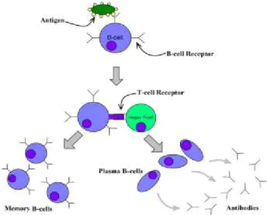
mechanisms allow for the localization and identification of the affected area, facilitating the concentration and effectiveness of defensive responses. The biological immune system is a naturally occurring adaptive control system that consists of specialized organs, cells, and chemical compounds whose ultimate objective is protecting the organism (the self) against harmful invading agents such as bacteria, viruses, and parasites (the non-self). The latter are generically referred to as antigens, while the specialized cells directly active in destruction are referred to as antibodies. Specialized immunity cells are generated based on the positive and negative selection, which attempt to ensure compatibility with the self and affinity to non-self, respectively. The immune system must first detect the presence of antigens by discriminating between self and non-self-based chemical markers that are present on the antigen’s surface but are not present on other cells. The number and virulence of the antigens can be assessed; thereby, facilitating the determination of the danger of the invasion. This evaluation of the situation is used to govern the humoral feedback mechanism which is responsible for controlling the generation of antibodies at levels required for destroying the antigen while using resources sparingly. The immune system comprises antibodies and lymphocytes. The two types of lymphocytes in the immune system are B-cells and T-cells. B-cells are produced in the bone marrow and used to recognize and eliminate antigens by generating antibodies. The thymus produces two types of T-cells, suppressing Ts-cells and assistant or helper Th-cells. The T-cells
are vital in regulating the production of B-cells and antibodies. If many antigens are detected, more Th-cells and fewer Ts-cells are produced, resulting in more B-cell production. As the
number of antigens present in the body decreases, the number of suppressing Ts-cells increases,
while Th-cells are reduced, ultimately leading to fewer B-cells and antibodies[24]. Eventually,
this process equalizes, and the immune response is complete. An overview of this process is presented in Figure 1.
Some of the immunity mechanisms have inspired the establishment of a framework by improving the capability for compensating errors of position and velocity estimation based on inertial measurement when GPS information or alternative sources are not available. Artificial memory cells are built as tandem collections of values of the system states and estimation errors or corrections. System state values are assimilated to the antigens because they are directly correlated to the estimation corrections, while the latter are assimilated to the antibodies. A positive selection type of mechanism must be used to select the proper memory cell by matching its state values to the current measured state. Once this is accomplished, the needed correction for the estimation scheme can be extracted from the artificial memory cell. This process is
equivalent to the detection of antigen by specialized immune cells and the use of memory B-cells for accelerated reaction through antibody generation. The AIS exhibits highly robust and
adaptive classification and information structuring capabilities, as well as memory and information fusion potential.
Figure 1. Immunity cell interactions.
3.2.Problem Formulation
An autonomous UAV is assumed to follow a commanded trajectory with disabled GPS feedback information. The measured states such as accelerations and angular rates are measured
on board by adequately functioning sensors to be used in the UAV velocity and position
estimation scheme. Through integration, the estimation errors accumulate over extended periods. The UAV would not achieve an adequate tracking performance because of such accumulative errors. It was hypothesized that an improvement of the trajectory tracking performance could be achieved by immediate estimated error corrections that depend on the short-term modification of vehicle dynamic state. The estimated corrections are assumed to be provided by the AIS. Within the AIS paradigm, the antigens represent the short-term state modifications, while antibodies represent the needed corrections. Therefore, the AIS construction consists of a collection of memory cells that associate to each configuration of dynamic system change, a set of
instantaneous estimation corrections. The variables that can be measured on-board must define the dynamic system state. When the measured velocity and position are available, the corrections can be determined in flight as an estimation error. For comprehensive usage of the approach, the AIS flight test construction must ideally cover all possible vehicle state configurations.
3.3.Definitions and Notations
3.3.1. The Aircraft (or UAV) Reference Frame and Coordinate System
The aircraft is assumed to be associated with the reference frame RFB and has a rigid
body and constant mass. The “body axes” are the aircraft Coordinate System (CS) and denoted as CSB or OXB YB ZB(see Figure 2). The origin O of the body axes is at the center of mass of the
aircraft. The longitudinal axis XB is along the fuselage with the positive direction forward in the
aircraft plane of symmetry with a direction at the discretion of the designer. YB is the lateral axis
positive to the right of the pilot and the vertical axis ZB is positive downward, as dictated by the
right-hand rule.
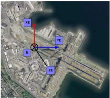
3.3.2. Earth Reference Frame and Coordinate System
The CS relative to the Earth is denoted as CSE or E XE YE ZE. The Earth is assumed to be
flat and inertial. E is the origin and established by the user on the interactive map of WVU UAS simulation environment. The initial location of the aircraft center of mass coincides with the origin E. XE is the longitudinal earth axis and selected to point up (towards North) with respect
to the simulation environment map. YE is the lateral axis and is in a positive direction to the right
(Eastwards). ZE is positive into the plan of the map as presented in Figure 3. The components of
the velocity vector 𝑣 with respect to 𝐶𝑆𝐸 (or 𝐸 𝑋𝐸 𝑌𝐸 𝑍𝐸) will be denoted as [𝑣 ]𝐸 =
[𝑣𝑥 𝑣𝑦 𝑣𝑧]𝐸𝑇.
Figure 3. Earth reference frame.
3.3.3. Euler Angles
Three Euler angles define the relative orientation of two CSs. Three rotations must be applied to obtain Euler angles successively along one axis at a time applied to one CS such that it eventually overlaps the second. The typical order of rotation starts with the vertical axis followed by the lateral and longitudinal axes [79]. For an aircraft, Euler angles represent the orientation of the fixed body axes with respect to a CS fixed in relationto the Earth. Euler angles are also referred to as aircraft attitude angles or angular position and denoted as roll, pitch, and yaw attitude angles (𝜑, 𝜃, 𝜓, respectively). With the most commonly used conventions, the roll attitude angle is positive if the aircraft is tilted to the right of the pilot, the pitch attitude angle is
positive if the aircraft is tilted nose-up, and the yaw attitude angle is positive if the nose of the aircraft points to the right of the pilot (see Figure 4).
Figure 4. Roll, pitch, and yaw rotation axes.
3.3.4. Transformation Matrix
When the coordinates for one CS are known, then the components or coordinates of a vector in relation to a different CS can be obtained using a transformation matrix. The
transformation matrix from 𝐶𝑆𝐸 to 𝐶𝑆𝐵 is denoted as 𝐿𝐵𝐸. The transformation matrices are orthonormal or 𝐿−1𝐵𝐸 = 𝐿𝑇𝐵𝐸. The elements of the transformation matrices are trigonometric functions of the Euler angles between the two CS.
[𝑣 ]𝐵 = 𝐿𝐵𝐸[𝑣 ]𝐸 = 𝐿−1𝐸𝐵[𝑣 ]𝐸 (4)
The transformation matrix from body axes components to Earth axes components is:
𝐿𝐸𝐵 = [
cos 𝜃 cos 𝜓 cos 𝜃 sin 𝜓 − sin 𝜃 sin 𝜙 sin 𝜃 cos 𝜓 − cos 𝜙 sin 𝜓 sin 𝜙 sin 𝜃 sin 𝜓 + cos 𝜙 cos 𝜓 sin 𝜙 cos 𝜃 cos 𝜙 sin 𝜃 cos 𝜓 + sin 𝜙 sin 𝜓 cos 𝜙 sin 𝜃 sin 𝜓 − sin 𝜙 cos 𝜓 cos 𝜙 cos 𝜃
3.3.5. Vector Derivative
Both variations in the magnitude and orientation of the vector 𝑣 must be taken into consideration; therefore, the derivative of a vector is defined in relation to the reference frame 𝑅𝐹𝐸 and denoted as:𝐸1𝑑𝑣⃗
𝑑𝑡 [80].
The relationship between the derivatives of the same vector with respect to two different RFs (𝑅𝐹𝐸 and 𝑅𝐹𝐵) is represented as:
𝑑 1 𝐸 𝑣 𝑑𝑡 = 𝑑 1 𝐵 𝑣 𝑑𝑡 + 𝜔⃗⃗ 1 𝐵 1 𝐸 × 𝑣 (6) where 𝜔⃗⃗ 1𝐵 1
𝐸 is the rotation vector of 𝑅𝐹
𝐵 with respect to 𝑅𝐹𝐸. 3.3.6. Position Vector
𝑝 𝐸𝑂 is the denotation of the position vector of the aircraft center of mass O with respect to a reference point on Earth, E. The UAV trajectory is defined by the position vector which is directed towards O and its origin is at point E. In other words, its components in 𝑅𝐹𝐸 are used to define the trajectory as follows:
[𝑝 𝐸𝑂] 𝐸 = [ 𝑥𝐸 𝑦𝐸 𝑧𝐸]𝐸 (7) 3.3.7. Velocity Vector 𝑣 1𝑂 1
𝐸 is the denotation of the translational velocity of the aircraft center of mass O with
respect to Earth reference frame 𝑅𝐹𝐸 and can be represented as follows: 𝑣 1𝑂 1 𝐸 = 1𝑑 𝐸 𝑝 𝐸𝑂 𝑑𝑡 (8) where 𝐸1𝑑.
𝑑𝑡 is the derivation operator with respect to 𝑅𝐹𝐸 and E can be any fixed point in 𝑅𝐹𝐸. The
components of 𝐸1𝑣 1𝑂 with respect to 𝑅𝐹𝐸 and 𝑅𝐹𝐵 are denoted as follows:
[ 𝑣 1𝑂 1 𝐸 ] 𝐸 = [ 𝑥̇𝐸 𝑦̇𝐸 𝑧̇𝐸 ] 𝐸 = [ 𝑣𝑥 𝑣𝑦 𝑣𝑧]𝐸,[ 𝑣 1 𝑂 1 𝐸 ] 𝐵 = [ 𝑢 𝑣 𝑤 ] 𝐵 , and [ 𝑣 1𝑂 1 𝐸 ] 𝐸 = 𝐿𝐸𝐵[ 𝑣 𝐸1 1𝑂]𝐵 (9)
3.3.8. Acceleration Vector
𝑎 1𝑂
1
𝐸 is the denotation of the translational acceleration of the aircraft center of mass 𝑂 with
respect to Earth reference frame 𝑅𝐹𝐸, as follows:
𝑎 1𝑂 1 𝐸 = 1𝑑 𝐸 𝑣 1𝑂 1 𝐸 𝑑𝑡 = 𝑑2 1 𝐸 𝑝 𝐸𝑂 𝑑𝑡2 (10) Also: 𝑎 1𝑂 1 𝐸 = 1𝑑 𝐸 𝑣 1𝑂 1 𝐸 𝑑𝑡 = 𝑑 1 𝐵 𝑣 1𝑂 1 𝐸 𝑑𝑡 + 𝜔⃗⃗ 1 𝐵 1 𝐸 × 𝑣 1𝑂 1 𝐸 (11) [ 𝑎 1𝑂 1 𝐸 ] 𝐸 = 𝐿𝐸𝐵{[ 𝑢̇ 𝑣̇ 𝑤̇ ] 𝐵 + [ 0 −𝑟 𝑞 𝑟 0 −𝑝 −𝑞 𝑝 0 ] 𝐵 [ 𝑢 𝑣 𝑤 ] 𝐵 } (12) where: [ 𝜔𝐸1⃗⃗ 1𝐵]𝐵 = [ 𝑝 𝑞 𝑟 ] 𝐵 (13) and : [ 𝑎 1𝑂 1 𝐸 ] 𝐸 = [ 𝑎𝑥 𝑎𝑦 𝑎𝑧]𝐸 (14) 3.3.9. Angular Position
The Euler angles [𝜑 𝜃 𝜓]𝑇 define the aircraft angular position or attitude. These are
the angles that define the relative orientation of 𝑅𝐹𝐵 or the aircraft rigid body with respect to 𝑅𝐹𝐸.
3.3.10.Angular Velocity Vector
The rotation of the aircraft as a rigid body (or equivalently 𝑅𝐹𝐵) with respect to the
denoted as 𝜔⃗⃗ 1𝐵 1
𝐸 . The components of the angular velocity vector are represented by equation (15)
are the result of three rotations about three non-perpendicular axes, consistent with the definition of Euler angles: 𝜔⃗⃗ 1𝐵 1 𝐸 = 𝜓̇⃗ + 𝜃̇ + 𝜑̇⃗ (15) Therefore: [ 𝑝 𝑞 𝑟 ] 𝐵 = [ 1 0 −𝑠𝑖𝑛(𝜃) 0 𝑐𝑜𝑠(𝜑) 𝑠𝑖𝑛(𝜑)𝑐𝑜𝑠(𝜃) 0 −𝑠𝑖𝑛(𝜑) 𝑐𝑜𝑠(𝜑)𝑐𝑜𝑠(𝜃) ] [ 𝜑̇ 𝜃̇ 𝜓̇ ] (16) and: [ 𝜑̇ 𝜃̇ 𝜓̇ ] = [ 1 𝑠𝑖𝑛(𝜑)𝑡𝑎𝑛(𝜃) 𝑐𝑜𝑠(𝜑)𝑡𝑎𝑛(𝜃) 0 𝑐𝑜𝑠(𝜑) −𝑠𝑖𝑛(𝜑) 0 𝑠𝑖𝑛(𝜑)/𝑐𝑜𝑠(𝜃) 𝑐𝑜𝑠(𝜑)/𝑐𝑜𝑠(𝜃) ] [ 𝑝 𝑞 𝑟 ] 𝐵 (17)
3.3.11.Angular Acceleration Vector
𝜔̇⃗⃗ 1𝐵
1
𝐸 vector represents the aircraft angular velocity and is invariant with respect to the
derivation RF because the cross product of a vector with itself is 0.
𝜔̇⃗⃗ 1𝐵 1 𝐸 = 1𝑑 𝐸 𝜔⃗⃗ 1𝐵 1 𝐸 𝑑𝑡 = 𝑑 1 𝐵 𝜔⃗⃗ 1 𝐵 1 𝐸 𝑑𝑡 (18) 3.3.12.Actual Values
The values of a variable that are reached by the real system are referred to as the actual values. Precisely, the actual values are not accessible because the only available access is to the measurements. To make this distinction, the actual values are referred to as the measurand values and are denoted with symbols without additional subscripts. For example, the actual position of aircraft will be designated by 𝑝 𝐸𝑂. In the simulation, actual values are obtained from the
mathematical model is rather of the system. To be more rigorous, the mathematical model is rather producing actual values plus modeling errors.
3.3.13.Measured Values
The sensor output values of a variable are represented as the measured values and denoted with symbols with subscript 𝑚. They are affected by measurement errors 𝑒 𝑚. For example, the measured position of the aircraft (e.g., provided by GPS) will be designated by 𝑝 𝑚𝐸𝑂 and:
𝑝
𝑚𝐸𝑂= 𝑝
𝐸𝑂+ 𝑒
𝑚 (1)3.3.14.Estimated Values
The estimation algorithms use limited sets of measurements, and the output values of a variable are represented as the estimated values and are denoted with symbols using subscript 𝑒. Estimation algorithms are affected by estimation errors 𝑒 𝑒 that are assumed to be the sum of estimation algorithm errors and measurement errors. For example, the estimated position of the aircraft will be designated by 𝑝 𝑒𝐸𝑂 and:
𝑝
𝑒𝐸𝑂= 𝑝
𝐸𝑂+ 𝑒
𝑒 (2)3.3.15.AIS-corrected Estimated Values
AIS-corrected estimations are the values obtained from the estimation scheme plus the corrections extracted from the AIS. For example:
𝑝
𝑐𝑒𝐸𝑂= 𝑝
𝑒𝐸𝑂+ 𝑝
𝐴𝐼𝑆𝐸𝑂 (3)3.3.16.Artificial Memory Cells
The Artificial Memory Cells (AMC) represent the AIS paradigm memory. The AMC mimic the T- and B-cells in the biological immune system, which stores information about antigen characteristics and the required antibodies for future accelerated and stronger immune response. AMCs are the building blocks of the AIS and consist of two parts: One including information on the characteristics of the system dynamic state referred to as “antigens” and one including the corresponding corrections for the estimation output, referred to as “antibodies.”
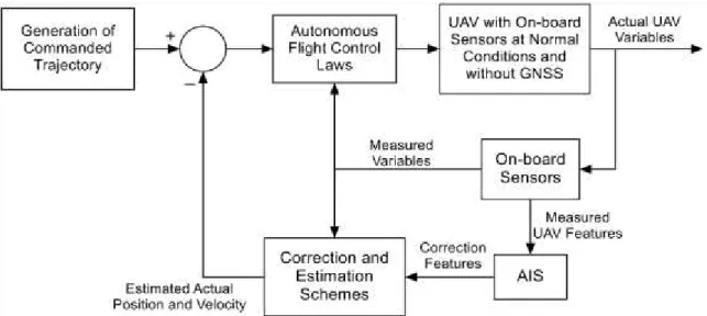
3.4.AIS-based Framework Architecture
The AIS-based framework relies primarily on two main processes:
i. Building the AIS which is performed “off-line” with data acquired during normal operation of the system.
ii. Extracting position and velocity estimation corrections from AIS and applying them,
which is performed “on-line,”when GPS is not working.
The AIS is envisioned as an information depository that relates states of aircraft with corrections needed for position and velocity estimations. Therefore, two sets of AIS features are needed:
i. The UAV features, including variables that define the dynamic state of the vehicle. ii. The correction features, including the variables that represent corrections needed for the
position and velocity estimations.
The estimation scheme of the position and velocity is assumed to operate adequately with information from on-board sensors, excluding GPS or alternative sources. Estimation scheme output is necessary both for the acquisition of data for AIS generation and during operation without GPS. The same level of performance of the estimation scheme is assumed in both situations.
3.4.1. The AIS Generation
The generation of the AIS consists of collecting and processing data under nominal conditions and structuring them as a set of artificial memory cells. Figure 5 presents the AIS building process. The main steps in this process are:
i. Definition of UAV and correction features.
ii. Design of tests for collecting data covering all possible dynamic configurations. iii. Execution of tests and data collection.
iv. Processing data for normalization and duplicate elimination.
v. AIS structuring as a table with two distinct areas for antibodies and antigens.
The following variables must be recorded for the commanded trajectory: i. Sensor measurements of UAV features.
ii. Estimated position and velocity produced by the on-board estimation scheme. iii. Measured position and velocity from GPS or other available sources.
Figure 5. Building the AIS (off-line).
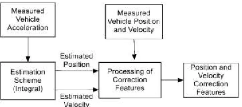
Two alternatives for structuring the AIS-based estimation correction process have been identified. One approach involves the correction of the output of the position and velocity estimation scheme (estimated vehicle position and velocity) and the other, the correction of the input of the estimation scheme (measured acceleration). The first approach will be referred to as
the “output” approach and the second, as the “input” approach. The two alternative solutions are illustrated in Figures 6 and 7 respectively.